Shrunken Locally Linear Embedding for Passive Microwave Retrieval of Precipitation

Abstract

This paper introduces a new Bayesian approach to the inverse problem of passive microwave rainfall retrieval. The proposed methodology relies on a regularization technique and makes use of two joint dictionaries of coincidental rainfall profiles and their corresponding upwelling spectral radiative fluxes. A sequential detection-estimation strategy is adopted, which basically assumes that similar rainfall intensity values and their spectral radiances live close to some sufficiently smooth manifolds with analogous local geometry. The detection step employs a nearest neighborhood classification rule, while the estimation scheme is equipped with a constrained shrinkage estimator to ensure stability of retrieval and some physical consistency. The algorithm is examined using coincidental observations of the active precipitation radar (PR) and passive microwave imager (TMI) on board the Tropical Rainfall Measuring Mission (TRMM) satellite. We present promising results of instantaneous rainfall retrieval for some tropical storms and mesoscale convective systems over ocean, land, and coastal zones. We provide evidence that the algorithm is capable of properly capturing different storm morphologies including high intensity rain-cells and trailing light rainfall, especially over land and coastal areas. The algorithm is also validated at an annual scale for calendar year 2013 versus the standard (version 7) radar (2A25) and radiometer (2A12) rainfall products of the TRMM satellite.

1 INTRODUCTION

From a mathematical standpoint, rainfall retrieval from remotely sensed observations is an inverse problem in which we aim to estimate the rainfall intensity from its indirect and noisy measurements. Passive retrieval of rainfall from upwelling spectral radiances is one of the most challenging atmospheric retrieval problems, chiefly because the rainfall spectral signatures are often downsampled, significantly corrupted with the background radiation and are non-linearly related to the rainfall vertical profile. Retrieval of rainfall from visible and infrared observations typically relies on empirical approaches as the measurements only respond to the radiative fluxes from the upper portion of the cloud layers [3, 6, 27, 1, 2, 36, 24, , among others]. In the microwave wavelengths ($\sim$ 6-to-200 GHz), the hydrometeor vertical profile is optically active and alters the upwelling radiations in the entire atmospheric column through absorption-emission and scattering processes. Over ocean, absorption-emission of the atmospheric liquid water can be well distinguished from the cold background by the physical laws of radiative transfer [e.g., 61, 35]. In addition, the attenuation of the polarized ocean surface emission by atmospheric hydrometeors [e.g., 46, 43, 44, 48, and references therein] and scattering by ice particles [e.g., 54, 35] also give rise to high signal-to-noise ratio in the rainfall spectral signatures making the retrieval problem more straightforward over ocean than over land. Over land, radiation from the highly emissive heterogeneous land surfaces often masks the hydrometeor emission signal enforcing the retrieval approaches to rely mostly on the complex scattering effects of the ice particles in the raining clouds [59, 47, 60]. As a result of these major differences over ocean and land, two classes of physically-based and empirical microwave retrieval algorithms have emerged. The empirical approaches have been predominantly used for retrieval over land while physically-based methods been used over ocean.

Over ocean, physically-based methods typically follow two distinct strategies. The first family of these algorithms [e.g., 61] simplifies the basic radiative transfer equation for atmospheric constituents under the axially symmetric scattering and Rayleigh-Jeans approximation. Given the observed spectral radiative fluxes with minimal scattering effect, the simplified equations permit to obtain atmospheric absorptivity, dropsize distribution and thus the rainfall intensity profile. The second class of methodologies [41, 40, 28, 45, 13, 29, 31, 32, among others], known as the Bayesian retrieval approaches, exploit a statistically representative a priori generated database that encodes the correspondence between the spectral brightness temperatures and rainfall profiles. In physically generated databases the causal relationships between the precipitation profiles and their upwelling spectral radiances are modeled using a combination of cloud resolving and radiative transfer models. Sophisticated numerical cloud resolving models (e.g., Goddard Cumulus Ensemble Model) are being used to produce a large collection of raining and non-raining cloud structures with distinct hydrometeor profiles. Then, for all of these profiles, a radiative transfer model is employed to obtain their spectral radiances at the top of the atmosphere. Finally, this database is utilized to retrieve rainfall profiles from observed microwave radiances using an inversion scheme. This approach has been the corner stone of the Goddard Profiling Algorithm GPROF [29, 31, 32] used to produce the TRMM operational passive retrieval products. On the other hand, over land, empirical methods typically rely on a scattering index [55, 21], which relates the depression in the high-frequency channels (e.g., 85 GHz) to the surface rainfall, in response to the frozen hydrometeors commonly found in the raining clouds. The magnitude of the high-frequency depression is naturally not independent of the land surface emissivity. As a result, prior to the rainfall estimation, different screening approaches are commonly employed to properly exclude depressions caused by the background noise (e.g., snow and desert surfaces). Among these, the early version of the GPROF [29, 31] suggests a static thresholding (22-85 GHz > 8 Kelvin) to detect raining signatures of the spectral brightness temperatures measured by the TRMM microwave imager (TMI). A more involved scattering index has also been suggested by Ferraro et al. [14, 16], which has been partly used to develop the launch version of the land retrieval algorithm for the Advanced Microwave Scanning Radiometer—Earth Observing System (AMSR-E) [60].

Upon successful launch of the TRMM satellite, a major body of research has also been devoted to developing rainfall retrieval algorithms by exploiting the coincidental observations provided by the TMI and TRMM precipitation radar (PR) [e.g., 42, 22, 37, 18, 20, 19, 53]. The basic idea has been focused on combining, in an optimal sense, the information content of both sensors for obtaining improved estimates of the rainfall profile and perhaps micro-physical properties of the atmospheric constituents. Typically, these methods use a variational cost function to reconcile the observations provided by both instruments [e.g., 18, 20, 19, 53], while recently Kummerow et al. [32] combined the PR data with the physically-driven database of the GPROF algorithm to make the database more observationally consistent. Using coincidental TMI and PR observations Petty and Li [48, 49] introduced a low-dimensional approximation method, using Principal Component Analysis (PCA), known as the University of Wisconsin (UW) algorithm. Specifically, Petty and Li [48] suggested a PCA based approach to project the nine TMI channels onto three pseudo channels for filtering the background noise and reducing redundancies in the TMI channels. These pseudo channels are then used within a matching process to efficiently recoPhysical retrievals of over-ocean rain rate from multichannel microwavever the surface rainfall from a compactly designed a priori database in a Bayesian context.

Passive rainfall retrieval remains a challenge especially for: 1) detection and estimation of the light rainfall over land and adjacent to coastlines, 2) unbiased estimation of rainfall over highly emissive and nonhomogeneous land surfaces, 3) probabilistic recovery of small-scale features of the rainfall extremes both over land and ocean [see, e.g., 38, 48, and references therein]. In this paper, motivated by these continuous challenges, we introduce a new Bayesian retrieval algorithm, called Shrunken Locally Linear Embedding for Retrieval of Precipitation (ShARP). This retrieval algorithm is guided by a priori collections of spectral radiances and their corresponding rainfall profiles, so-called spectral and rainfall “dictionaries”. The core part is inspired by the concept of locally linear embedding [50], which assumes that “similar” spectral radiances and their corresponding rainfall profiles live close to two joint smooth manifolds allowing locally linear approximations. To retrieve rainfall, ShARP uses a $k$-nearest neighborhood classification (detection step) coupled with a modern shrinkage regularization scheme (estimation step). For an observed spectral radiance, the detection step finds similar signatures in the spectral dictionary and decides whether the observed spectral radiance is non-raining or raining. For a raining spectral radiance, the estimation step uses a shrinkage estimator to obtain its representation coefficients in the spectral dictionary. Then, the representation coefficients are used to combine the corresponding rainfall profiles from the rainfall dictionary to result in the rainfall retrieval.

In summary, the main contribution and advantageous features of this algorithm for addressing the aforementioned retrieval challenges are: 1) The use of supervised nearest neighborhood classification results in minimal sensitivity to the variability of the underlying land surface emissivity. This property promises improved retrieval over troublesome surfaces and coastal zones. 2) The core estimation step makes use of a modern constrained regularization scheme giving rise to sufficiently stable retrievals with reduced error, compared to the classic least-squares solutions. 3) By design and due to the used regularization scheme, the algorithm is flexible and robust enough to employ dictionaries populated either empirically or via physically-based modeling or a combination of them. 4) The algorithm allows us to approximate the posterior probability density function of the retrieved rainfall, especially useful for hazard assessment of the rainfall extremes and their hydro-geomorphic impacts. It is important to note that the current implementation of our algorithm is fully empirical, as we populate the rainfall and spectral dictionaries only with the coincidental observations of the TRMM-PR and TMI. Therefore, in the absence of any independent ground-based validation, all of the presented retrieval results are bounded by accuracy of the PR sensor/algorithm [see, 4]. Clearly, as we validate our results with the 2A25, improved retrievals often do not come as a surprise; however, they remain of significant importance as currently the passive retrieval methods are empirical over land and coastal areas.

Section 2 is devoted to explaining the rainfall dataset and studying the rainfall spectral patterns relevant to the design of the presented algorithm. Section 3 explains the details of the ShARP algorithm. Using the TRMM data, in Section 4, some retrieval results are presented and compared with the currently operational PR-2A25 and TMI-2A12 retrieval products (version 7). Conclusions are drawn and future lines of research are pointed out in Section 5.

2 TRMM Rainfall Database

Before we embark upon a detailed algorithmic discussion, we provide a brief explanation of the dataset used and some relevant insights into the structure of raining and non-raining microwave spectral patterns, which are essential to the development of our algorithm.

The TRMM-PR is a Ku band radar that operates in a single polarization mode at frequency 13.8 GHz. Currently, the PR provides direct measurements of rainfall reflectivity at grid size 4-to-5 km over a swath width of 247 km and samples the first 15 to 20 km of the troposphere at every ~250 m at nadir. On the other hand, TMI is a dual-polarized multichannel radiometer that operates on central frequencies 10.65, 19.35, 21.3, 37.0, and 85.5 GHz. All of the channels are horizontally and vertically polarized except the vertical water vapor channel 21.3 GHz. Currently, TMI provides spectral brightness temperatures over a swath width of 878 km with nominal spatial resolution greater than 5.1 km at 85.5 GHz. By design, the TMI and PR sensors provide overlapping observations over the inner swath within the radar field of view at different resolutions. A thorough exposition of the TRMM sensor packages can be found in [30].

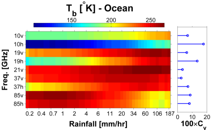
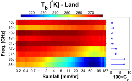
Figure 1: Expected values of the spectral brightness temperatures for different intervals of the surface rainfall intensity over ocean (left panel) and land (right panel). The images are inferred from coincidental pairs of the TMI-1B11 and PR-2A25 products obtained from 1000 randomly chosen orbits in our rainfall database. The stem plots demonstrate the coefficients of variation for each spectral band in response to the underlying rainfall variability. Note that, the rainfall intervals on the x-axis are logarithmically spaced between 0.2 to 200 mm/hr.

Here, we use the coincidental 2A25 (level-II) product of the radar profiling algorithm [25] and the 1B11 (level-I) product of the radiometer to construct the rainfall and spectral dictionaries. To register all of the data onto a single grid of latitude/longitude, we simply used the nearest neighborhood interpolation and mapped the TMI spectral temperatures onto the reported PR grids. Note that in this case, we neither loose nor add any information and retrieve rainfall at the native resolution of the 1B11 at the high-frequency channel 85 GHz. Clearly, in this resolution, the lower frequency channels provide redundant spectral information over neighboring grid-boxes while their combinations with higher frequency channels may still provide distinct multi-spectral information. Accordingly, throughout this paper, we use a large collection of collocated TMI and PR data, hereafter called “rainfall database”, over the TRMM inner swath for all orbital tracks in calendar years 2002, 2005, 2008, 2011, and 2012.

Using the collected rainfall database, Fig. 1 shows the conditional expectations of the TMI spectral brightness temperatures for different ranges of the PR rainfall intensities as well as their coefficients of variation. Specifically, each column of the shown images demonstrates the conditional mean of the TMI channels, while each row shows the average response of the channels to the underlying rainfall variability. On the other hand, the stem plots represent the coefficients of variation of the brightness temperatures for each channel. Over ocean (left panel), we see that almost all frequencies are relatively responsive to the underlying surface rainfall variability. Horizontal channels of 10 and 19 GHz show the maximum normalized variations, while the vertical polarizations in frequencies of 21 and 37 GHz are the least responsive channels. This observation is consistent with the fact that ocean surface is less emissive in horizontal polarizations for the TMI view angle, giving rise to colder background and thus larger signal-to-noise ratio of the raining signatures [58]. On the contrary, over land, almost all of the low-frequency channels below 21 GHz show relatively small coefficients of variation compared to the higher frequencies. It will be clear later on that these coefficients of variation can be used to properly weight each channel to better guide the proposed retrieval approach.

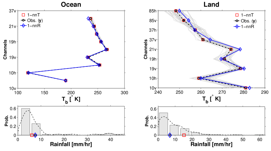
Figure 2: Top panels: Two arbitrary sampled raining vectors of the TMI-IB11 spectral brightness temperatures (dotted black lines with circles) over ocean (left) and land (right). The gray lines are the 50-nearest spectral neighbors in the Euclidean sense, obtained from an independent learning set of the TMI-1B11 observations. Bottom panels: PR-2A25 surface rainfall probability histograms of the 50 spectral neighbors, shown in the top panels. In top and bottom panels, the red squares and the blue solid lines with diamonds show the 1-nearest neighbor in the spectral (1-nnT) and rainfall (1-nnR) spaces, respectively.

Furthermore, to better understand the correspondence between the neighboring raining spectral brightness temperatures, in the Euclidean sense, and their surface rainfall intensities, we independently collected two learning sets of the form $\mathcal{L}=\left\{\left(\mathbf{b}_{i},\,r_{i}\right)\right\}_{i=1}^{M}$ over ocean and land. Each set contains $M\approxeq 10^{6}$ of coincidental 1B11 spectral brightness temperatures $\mathbf{b}\in\mathfrak{R}^{9}$ and their corresponding 2A25 surface rainfall $r\in\mathfrak{R}$ estimates. From a mathematical stand point, a simple nearest neighborhood search reveals that the spectral temperatures over ocean and land are not uniquely related to the estimated surface rainfall intensities in the Euclidean sense [see, 33, for more discussion]. Nevertheless, in the known lack of uniqueness, a basic question arises: How can we obtain “stable” estimates of the surface rainfall using neighboring spectral brightness temperatures in a properly collected learning set? To this end, let us assume that a spectral vector of brightness temperature is denoted by $\mathbf{y}$ and its scalar surface rainfall value of interest is $x$. Top panels from left to right in Fig. 2 demonstrate two arbitrary vectors of the 1B11 raining brightness temperatures $\mathbf{y}\in\mathfrak{R}^{9}$ (black dashed lines) over ocean and land, together with their fifty nearest neighbors $\left\{\mathbf{b}_{k}\left(\mathbf{y}\right)\right\}_{k=1}^{K=50}$ (gray solid lines) obtained from the collected learning sets. Bottom panels show the corresponding surface rainfall values $\left\{r_{k}\left(\mathbf{y}\right)\right\}_{k=1}^{K=50}$ and their probability histograms. It turns out that all of the fifty nearest spectral brightness temperatures were raining except for only one of them over land. This observation implies that a supervised nearest neighborhood classification, using coincidental TMI and PR data, might be a very powerful approach for the rain/no-rain discrimination problem. Furthermore, it can be seen that the first nearest neighbor in the spectral space (1-nnT) does not necessary relate to the nearest neighbor (1-nnR) in the rainfall space. However, in both cases, the surface rainfalls of the neighboring spectral vectors are bounding the rainfall values $x$ of interest. These bounds, both in the spectral and rainfall spaces, are clearly tighter over ocean than over land, mainly due to the stronger signal to noise ratio of the rainfall signatures. Therefore, for each sampled $\mathbf{y}$, it can be naturally concluded that a properly chosen statistic of $\left\{r_{k}\left(\mathbf{y}\right)\right\}_{k=1}^{K}$ in the following form

$$\hat{x}=\sum_{k=1}^{K}c_{k}\,r_{k}\left(\mathbf{y}\right),$$ (1)

may be adopted as a stable estimator of $x$, where $c_{k}$ denotes some optimal weighting coefficients.

3 SHRUNKEN LOCALLY LINEAR EMBEDDING FOR RETRIEVAL OF PRECIPITATION

3.1 Rainfall Retrieval as an Inverse Problem

Passive rainfall retrieval in the microwave bands can be considered as a nonlinear inverse problem, where its solution shall be constrained by the underlying laws of atmospheric thermal radiative transfer in a weak or strong sense [e.g., 26, 52]. To recast the microwave rainfall retrieval in a standard form of a discrete inverse problem, let us assume that each vector of spectral brightness temperatures and their corresponding rainfall profiles are $\mathbf{y}=\left(y_{1},y_{2},\ldots,y_{n_{c}}\right)^{{\rm T}}$ and $\mathbf{x}=\left(x_{1},x_{2},\ldots,x_{n_{r}}\right)^{{\rm T}}$, respectively, where $n_{c}$ and $n_{r}$ denote the number of spectral channels and vertical layers of the rainfall intensity profile. As a result, in a finite dimension, spectral observations might be related to the rainfall intensity profile through the following nonlinear observation model:

$$\mathbf{y}=\mathcal{F}\left(\mathbf{x}\right)+\mathbf{v},$$ (2)

where, $\mathcal{F}\left(\cdot\right):\,\mathbf{x}\rightarrow\mathbf{y}$ can be considered to be a functional representation of the radiative transfer equations that maps the rainfall intensity profiles onto the space of spectral brightness temperatures, and $\mathbf{v}\in\mathfrak{R}^{n_{c}}$ represents the observation error with a finite energy. Obviously, the goal of the retrieval is to obtain an estimate of the rainfall profile $\mathbf{x}$, given spectral brightness temperatures $\mathbf{y}$, the radiative transfer functional $\mathcal{F}\left(\cdot\right)$, and a priori information about the error. The search for a stable closed form solution of the above inverse problem seems almost a hopeless quest at least for now, given the fact that $\mathcal{F}\left(\cdot\right)$ is extremely nonlinear, especially under the scattering dominant regime. In the subsequent section it will be clear that our algorithm is indeed a workaround to this complex inverse problem.

3.2 Algorithm

Motivated by our observations in Section 2, to bridge the explained complexities in the rainfall retrieval problem, our algorithm relies on a priori collected database or say learning set denoted by $\mathcal{L}=\left\{\left(\mathbf{b}_{i},\,\mathbf{r}_{i}\right)\right\}_{i=1}^{M}$. This set is populated by a large number of coincidental brightness temperatures $\mathbf{b}_{i}=\left[b_{1i},b_{2i},\ldots,b_{n_{c}i}\right]^{{\rm T}}\in\mathfrak{R}^{n_{c}}$ and their corresponding rainfall profiles $\mathbf{r}_{i}=\left[r_{1i},r_{2i},\ldots,r_{n_{r}i}\right]^{{\rm T}}\in\mathfrak{R}^{n_{r}}$. For notational convenience, let us stack these pairs according to a fixed order in two joint matrices $\mathbf{B}=\left[\mathbf{b}_{1}|\ldots|\mathbf{b}_{M}\right]\in\mathfrak{R}^{n_{c}\times M}$ and $\mathbf{R}=\left[\mathbf{r}_{1}|\ldots|\mathbf{r}_{M}\right]\in\mathfrak{R}^{n_{r}\times M}$, which are called the spectral and rainfall “dictionaries”. In our notation, each of these pairs are called elementary “atoms” to be used for reconstruction of the rainfall fields from their observed spectral signatures. As is evident, theses dictionaries can be populated either by observational or physically-based generated pairs.

In the detection step, we simply use a supervised nearest neighborhood classification rule, guided by the dictionaries. In particular, for a given observation vector of spectral brightness temperature $\mathbf{y}\in\mathfrak{R}^{n_{c}}$ and the dictionary pair $\left(\mathbf{B},\,\mathbf{R}\right)$, let us assume that $\mathcal{S}$ denotes the set of $K$ column indices of $\mathbf{B}$ that contain the nearest spectral atoms to $\mathbf{y}$ in the Euclidean sense. Given this set, the algorithm forms two joint sub-dictionaries $\left(\mathbf{B}_{\mathcal{S}}\in\mathfrak{R}^{n_{c}\times K},\>\mathbf{R}_{\mathcal{S}}\in\mathfrak{R}^{n_{r}\times K}\right)$, which are generated by those $K=\left|\mathcal{S}\right|$ nearest spectral $\left\{\mathbf{b}_{k}\right\}_{k=1}^{K}\in\mathbf{B}$ and their corresponding rainfall atoms $\left\{\mathbf{r}_{k}\right\}_{k=1}^{K}\in\mathbf{R}$. Assuming that the last row of the rainfall sub-dictionary $\mathbf{R}_{\mathcal{S}}$ contains the near surface rainfall intensity values, the algorithm simply makes use of a probabilistic voting to declare $\mathbf{y}$ as raining or non-raining. In other words, choosing a probability threshold $p$, the algorithm labels $\mathbf{y}$ as raining, if more than $p\,K$ number of $\left\{\mathbf{r}_{k}\right\}_{k=1}^{K}$ are raining at the surface. In the estimation step, motivated by the results in Fig. 2, we assume that the true rainfall profile $\mathbf{x}$ of the given spectral observation $\mathbf{y}$ can be well explained by the $\mathbf{R}_{\mathcal{S}}$’s atoms, through the following linear model:

$$\mathbf{x}=\mathbf{R}_{\mathcal{S}}\mathbf{c}+\mathbf{e},$$ (3)

where $\mathbf{c}\in\mathfrak{R}^{K}$ is a vector of representation coefficients that linearly combines atoms of the rainfall sub-dictionary and $\mathbf{e}\in\mathfrak{R}^{n_{r}}$ denotes a zero mean error with finite energy. As a result, given an estimate of the representation coefficients $\hat{\mathbf{c}}$, conditional expectation of the rainfall profile $\hat{\mathbf{x}}$ can be obtained as follows:

$$\hat{\mathbf{x}}=\mathbb{E}\left(\mathbf{x}|\hat{\mathbf{c}}\right)=\mathbf{R}_{\mathcal{S}}\hat{\mathbf{c}}.$$ (4)

Obviously, estimation of the representation coefficients solely from equation (3) is ambiguous as both sides of the equation are unknown. To find a solution, as previously explained, we assume that the neighboring rainfall profiles and their spectral signatures live close to two smooth manifolds with analogous geometric structure and thus similar locally linear representation. Therefore, the algorithm assumes a spectral observation model with the same linear representation coefficients as follows:

$$\mathbf{y}=\mathbf{B}_{\mathcal{S}}\mathbf{c}+\mathbf{v},$$ (5)

where $\mathbf{v}\in\mathfrak{R}^{n_{c}}$ denotes a zero mean error with finite energy. As is evident, estimation of the representation coefficients from (5) is no longer an ill-defined problem. To estimate the representation coefficients in this linear model, the weighted Minimum Mean Squared Error (MMSE) estimator, constrained to the probability simplex, seems to be the first choice as follows:

$$\underset{\mathbf{c}}{\text{minimize}} \left\|\mathbf{W}^{1/2}\left(\mathbf{y}-\mathbf{B}_{\mathcal{S}}\mathbf{c}\right)\right\|_{2}^{2}$$ (6)

subject to $$\mathbf{c}\succeq 0,\enskip\mathbf{1}^{{\rm T}}\mathbf{c}=1,$$

where the $\ell_{2}$-norm is $\left\|\mathbf{c}\right\|_{2}^{2}=\Sigma_{i}c_{i}^{2}$, $\mathbf{c}\succeq 0$ implies element-wise non-negativity and the positive definite $\mathbf{W}\succ 0$ in $\mathfrak{R}^{n_{c}\times n_{c}}$ determines the relative importance or weights of each channel. These weights may be chosen to relatively encode the signal-to-noise ratio of the spectral raining signatures. Note that the non-negativity constraint is required to be physically consistent with the positivity of the brightness temperatures in Kelvin. Furthermore, the sum to one constraint assures that the estimates are locally unbiased. More importantly, this equality constraint makes the solution invariant to rotation, rescaling, and translation of the neighboring spectral observations [see, 50]. For similar concept in rainfall downscaling, the reader is also referred to [10] and [17].

However, problem (6) is likely to be severely ill-posed due to the observation noise, especially when the column dimension of $\mathbf{B}_{\mathcal{S}}$ is larger than that of spectral bands $n_{c}$. To make the problem well-posed and sufficiently stable, we suggest the following regularization scheme

$$\underset{\mathbf{c}}{\text{minimize}} \left\|\mathbf{W}^{1/2}\left(\mathbf{y}-\mathbf{B}_{\mathcal{S}}\mathbf{c}\right)\right\|_{2}^{2}+\lambda_{1}\left\|\mathbf{c}\right\|_{1}+\lambda_{2}\left\|\mathbf{c}\right\|_{2}^{2}$$ (7)

subject to $$\mathbf{c}\succeq 0,\enskip\mathbf{1}^{{\rm T}}\mathbf{c}=1,$$

where the $\ell_{1}$-norm is $\left\|\mathbf{c}\right\|_{1}=\Sigma_{i}\left|c_{i}\right|$, $\lambda_{1},\,\lambda_{2}$ are non-negative regularization parameters. Obviously, obtaining $\hat{\mathbf{c}}$ as the solution of the above problem, we can retrieve the rainfall using expression (4) as $\hat{\mathbf{x}}=\mathbf{R}_{\mathcal{S}}\hat{\mathbf{c}}$.

Input: Spectral observations $\mathbf{Y}$ containing $\left\{\mathbf{y}_{i}=\left[y_{1i},y_{2i},\ldots,y_{n_{c}i}\right]^{{\rm T}}\in\mathfrak{R}^{n_{c}}\right\}_{i=1}^{N}$ vectors of spectral brightness temperatures, spectral $\mathbf{B}\in\mathfrak{R}^{n_{c}\times M}$and rainfall $\mathbf{R}\in\mathfrak{R}^{n_{r}\times M}$ dictionaries, weight matrix $\mathbf{W}\in\mathfrak{R}^{n_{c}\times n_{c}}$, detection probability $p$, number of nearest neighborhoods $K$, and regularization parameters $\lambda_{1}$, $\lambda_{2}$.

Output: Precipitation field $\mathbf{X}$ containing $\left\{\mathbf{x}_{i}\in\mathfrak{R}^{n_{r}}\right\}_{i=1}^{N}$ pixels of rainfall intensity profiles.

For $i:=1$ to $N$ step 1 do

• Find sub-dictionaries $\mathbf{B}_{\mathcal{S}}\in\mathfrak{R}^{n_{c}\times K}$ and $\mathbf{R}_{\mathcal{S}}\in\mathfrak{R}^{n_{r}\times K}$, where $\mathcal{S}$ is the set of column indices of $\mathbf{B}$ which contains the $k$-nearest neighborhoods of $\mathbf{y}_{i}$.

• Let $\mathbf{R}_{\mathcal{S}}\left(\text{end},\,:\right)$ denotes the last row of $\mathbf{R}_{\mathcal{S}}$ containing neighboring surface rainfall.

• If $\left|{\rm supp}\left(\mathbf{R}_{\mathcal{S}}\left(\text{end},\,:\right)\right)\right|\geq p\,K$ ,
  
   - Standardize $\mathbf{y}_{i}$ and atoms of $\mathbf{B}_{\mathcal{S}}$, such that $\sum_{j}^{n_{c}}y_{ji}=0$ , $\sum_{j}^{n_{c}}b_{jk}=0$ , and $\sum_{j}^{n_{c}}b_{jk}^{2}=1$ , for $k=1,\ldots,K$.
   - $\hat{\mathbf{c}}_{i}={\rm argmin}_{\mathbf{c}_{i}\succeq 0,\>\mathbf{1}^{{\rm T}}\mathbf{c}_{i}=1}\left\{\left\|\mathbf{W}^{1/2}\left(\mathbf{y}_{i}-\mathbf{B}_{\mathcal{S}}\mathbf{c}_{i}\right)\right\|_{2}^{2}+\lambda_{1}\left\|\mathbf{c}_{i}\right\|_{1}+\lambda_{2}\left\|\mathbf{c}_{i}\right\|_{2}^{2}\right\}$
   - $\hat{\mathbf{x}}_{i}=\mathbf{R}_{\mathcal{S}}\hat{\mathbf{c}}_{i}$
  
  else
  
   - $\hat{\mathbf{x}}_{i}=0$
  
  End If

End For

Algorithm 1 Shrunken Locally Linear Embedding Algorithm for Retrieval of Precipitation (ShARP).

Note that problem (7) is a non-smooth convex problem. It is non-smooth as the $\ell_{1}$-norm is not differentiable at the origin. Convexity arises as it uses a conic combination of two well-known convex penalty functions to regularize a classic weighted least-squares problem over a convex set. These two regularization functions have been widely used to properly narrow down the solution of ill-posed inverse problems. In under-determined system of equations, the $\ell_{1}$-norm penalty has proven to be an effective regularization for obtaining “sparse” solutions. In other words, it turns out that this regularization promotes sparsity in the solutions, as it uses a minimal number of atoms of $\mathbf{B}_{\mathcal{S}}$, while retains maximum amount of information [9, 56, 8, 11]. On the other hand, the $\ell_{2}$-norm penalty is the most widely used regularization approach to stabilize the solutions of “dense” ill-posed inverse problems while it incorporates all the atoms of $\mathbf{B}_{\mathcal{S}}$ [57, 23] in the solution. Confining the regularization in (7) solely to the $\ell_{1}$-norm ($\lambda_{2}=0$) is restrictive for rainfall retrieval in the current setting of our algorithm because of two main reasons. First, the number of selected columns of $\mathbf{B}_{\mathcal{S}}$, or say non-zero elements of the representation coefficients, will be bounded in this case by the number of the available spectral bands $n_{c}$. Second, the spectral atoms in the sub-dictionary $\mathbf{B}_{\mathcal{S}}$ are likely to be highly correlated and clustered in groups. In this condition, the $\ell_{1}$-norm regularization typically fails to take into account the contribution of clustered atoms. On the other hand, all of the spectral atoms in $\mathbf{B}_{\mathcal{S}}$ will be taken into account if we solely rely on the $\ell_{2}$ penalty, which can lead to selection of irrelevant atoms and overly smooth rainfall retrieval. However, the proposed mixed penalty removes the explained limitations of each individual regularization scheme through stabilizing the problem regularization path, encouraging grouping effects by shrinking the clusters of correlated atoms and averaging their representation coefficients [see, 64]. In addition, from a practical point of view, this mixed regularization increases the flexibility of the algorithm to cope with the ill-conditioning arising due to the presence of very similar and correlated atoms in the spectral sub-dictionary. This property is extremely desirable especially for the future developments of our algorithm to accommodate both observationally and physically generated dictionaries. Throughout this paper, we consider a convex combination of regularization penalty functions by assuming $\lambda_{2}=\lambda\alpha$ and $\lambda_{1}=\lambda\left(1-\alpha\right)$ for all $\alpha\in\left(0,\,1\right)$. As we use the concept of locally linear embedding together with the above mixed shrinkage estimation, we call our retrieval technique the Shrunken Locally Linear Embedding Algorithm for Retrieval of Precipitation (ShARP). The details are summarized in Algorithm 1 and sketched in Fig. 3. Given the induced non-negativity constraint in problem (7) allows us to solve it via a constrained quadratic programming (QP) as follows:

$$\underset{\mathbf{c}}{\text{minimize}} \mathbf{c}^{{\rm T}}\left(\mathbf{B}_{\mathcal{S}}^{{\rm T}}\mathbf{W}\mathbf{B}_{\mathcal{S}}+\lambda_{2}\mathbf{I}\right)\mathbf{c}+\left(\lambda_{1}\mathbf{1}-\mathbf{B}_{\mathcal{S}}^{{\rm T}}\mathbf{W}^{{\rm T}}\mathbf{y}\right)^{{\rm T}}\mathbf{c}$$ (8)

subject to $$\mathbf{c}\succeq 0,\enskip\mathbf{1}^{{\rm T}}\mathbf{c}=1,$$

where $\mathbf{1}=\left[1,\ldots,1\right]^{{\rm T}}\in\mathfrak{R}^{K}$.

Figure 3: Flowchart of the ShARP algorithm. See Algorithm 1 for more detailed explanation.

It is important to note that problem (7) is, in effect, a constrained Bayesian Maximum a Posteriori (MAP) estimator under the following prior

$$p\left(\mathbf{c}\right)\propto\exp\left(-\lambda_{1}\left\|\mathbf{c}\right\|_{1}-\lambda_{2}\left\|\mathbf{c}\right\|_{2}^{2}\right),$$ (9)

which is a conic combination of the Gaussian and Laplace densities [see, 63]. Therefore, the posterior density of the estimated coefficients and thus rainfall values is not Gaussian. As a result, closed form uncertainty analysis of the retrieved rainfall is not trivial and may be addressed through randomization or ensemble analysis. To this end, one can simply see that the rows of the sub-dictionary $\mathbf{R}_{\mathcal{S}}$ contain $K$-samples of the posterior Probability Density Function (PDF) of the neighboring rainfall intensity profiles. Thus, depending on the selected number of the nearest neighbors, the whole posterior PDF of the ShARP estimator can be empirically approximated by counting the relative frequency of the rainfall occurrence. This strategy will be used in the sequel to estimate the uncertainty of the retrieved rainfall.

4 EXPERIMENTS USING TRMM DATA

As previously explained, in the current implementation of ShARP, we only confine our consideration to empirical rainfall and spectral dictionaries collected from the coincidental PR-2A25 and TMI-1B11 products and only retrieve surface rainfall. Therefore, the 2A25 product can be used as a reference to validate the results of the ShARP algorithm. To further examine the pros and cons of its performance, all of the retrieval experiments are also shown versus the surface rainfall obtained from the standard passive TMI-2A12 retrieval product.

4.1 Algorithm Setup

In the current implementation of ShARP, we defined four different earth surface classes, namely: ocean, land, coast and inland water (Fig. 4). In other words, we collected four dictionaries over each surface class and use them in Algorithm 1 depending on the geolocation of a given pixel of the observed spectral brightness temperatures. This surface stratification is obtained from standard surface data in the PR-1C21 product (version 7) at $\sim 5\times 5$ km grid box. In this classification, the coastal areas are referred to those locations on the globe, where the presence of water is not permanent due to the seasonal variations or tidal effects. To construct spectral and rainfall dictionaries, we randomly sampled 750 orbits from our rainfall database. In these sampled orbits, more than $25\times 10^{6}$ pairs of raining and non-raining signatures were used to construct the required dictionaries.

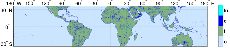
Figure 4: Different earth surface classes used in the current version of the ShARP, namely inland water body (In), coastal zone (c), land (l) and ocean (o). The classification is adopted based on the available data (version 7) of the PR-1C21 product, which are mapped onto a $0.05$-degree regular grid.

4.1.1 Detection Step

As previously explained, rain/no-rain classification from microwave observations and its induced error on the quality of rainfall retrieval has been addressed in numerous studies [e.g., 21, 28, 34, 15, 51], and reported as a challenging problem which is not easy to mitigate, especially over land [see, 32]. Therefore, in developing rainfall retrieval techniques, we naturally have a choice to either first detect the storm raining areas and then estimate the rainfall intensities or just use an estimation scheme that automatically recovers the raining areas. In general, rainfall retrieval with a sequential rain/no-rain detection and estimation scheme may be advantageous in the sense that it allows us to control the probability of false alarm while confining the computational expense of estimation only to the detected raining areas.

Considering 2A25 as a reference rainfall field to validate ShARP, Fig. 5 shows the estimated probability of hit (${\rm Pr}_{{\rm H}}$) versus probability of false alarm (${\rm Pr}_{{\rm F}}$) for the rain/no-rain detection step of our algorithm as the classification parameters are varied. Here, the results are obtained by applying the detection step to more than $3\times 10^{5}$ randomly chosen pixels of spectral observations from our rainfall database. Note that, these spectral pixels are selected randomly from our rainfall database and have not been used in the construction of the retrieval dictionaries. In Fig. 5, we can see that the ShARP classification rule is not very sensitive to the number of chosen nearest neighborhoods as all of the curves are nearly collapsing onto each other. The ShARP rain/no-rain detection quality for $K=20$ and the majority vote rule, that is $p=0.5$, is presented in Table 1. This table explains that over ocean and land, our algorithm matches raining pixels of the 2A25 in 96 and 90% of the cases while the false alarm rate does not exceed 8% and 6%, respectively. Fig. 5 also shows the position of the 2A12 retrieval product. It is seen that, given the 2A25 is raining over ocean, the 2A12 is raining in 95% of the cases. On the other hand, we see that in 20% of the cases 2A12 detects raining areas which may have been missed by the 2A25 and thus ShARP. Although interpretation of this discrepancy is not central to the thrust of this paper, this result seems to be consistent with the recent evidence from the CloudSat satellite suggesting that the PR underestimates the extent of light rain over ocean [12], which may reach up to 10% of the rainfall volume on average over the tropics [5]. Conversely, over land, we see that if 2A25 is raining, ShARP is raining in 90% of cases while 38% of these raining pixels are not captured in the 2A12.

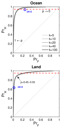
Figure 5: Rainfall Receiver Operating Characteristic (ROC) curve over ocean top panel) and land (bottom panel) for different probability of detection $p\in[0,\,1]$ and number of nearest neighborhoods $K\in\left\{5,\,10,\,20,\,40,\,100\right\}$ of the ShARP algorithm. The blue circles show the 2A12 (version 7) product and the red dash-dotted lines show the 0.95 probability of hit as a datum.

		Observation (2A25)
		Ocean		Land
		rain	no-rain	rain	no-rain
Detection (ShARP)	rain	0.96	0.08	0.90	0.06
	no-rain	0.04	0.92	0.1	0.94

Table 1: Probability of hit and false alarm for twenty nearest neighbors $K=20$ and probability threshold of $p=0.5$. The results are obtained by comparing ShARP with 2A25.

4.1.2 Estimation Step

After finding the storm raining areas, our algorithm moves toward estimation of the rainfall intensities. Recall that, we use a positive definite weight matrix $\mathbf{W}$ in problem (7) that determines the relative importance of each channel over different surface classes. To design this weight matrix, we use the normalized coefficients of variation for each channel as reported in Fig. 1. In particular, the relative weight of the $i^{\text{th}}$ channel for a specific surface class is obtained by normalizing its coefficient of variation as $w_{i}=c_{v}^{i}/\underset{i}{\max}\left(c_{v}^{i}\right)$, $i=1,\,\ldots,\,9$ (Table 2). The weight matrix is then assigned to be $\mathbf{W}=\text{diag}\left(w_{i}\right)$. Using these weights allows us to make the least-squares term in problem (7) invariant to temperature translations among spectral channels and more responsive to stronger rainfall signal-to-noise ratio. In other words, these weights reduce saturation of the cost due to some excessively cold and/or warm channels while maintain it sensitive to their relative variability. To solve problem (7), we use a primal-dual interior-point method [see, 7, chap. 11]. Basically, in this class of convex optimization techniques, the inequality constrained quadratic programing problem (8) is reformulated into an equality constrained problem to which iterative Newton’s method can be applied. Specifically, we employed Linear-programing Interior Point SOLver (lIPSOL) [62] which is based on a variant of the algorithm by Mehrotra [39]. In this optimization sub-algorithm the maximum number of iterations in Newton’s steps is set to 200, the termination tolerance on the function value and magnitude of relative changes in the optimization variable are both set to $1\text{e}-8$. We set the algorithm regularization parameters to be $\lambda=0.001$ and $\alpha=0.1$, which appears to work well for a wide range of rainfall retrieval experiments. This setting permits the algorithm to perform a full orbital rainfall retrieval in the order of 10 to 15 minutes on a contemporary desktop machine.

Relative weights
Surface Classes	Channels
	10v	10h	19v	19h	21v	37h	37v	85v	85h
Ocean	0.39	1.00	0.35	0.76	0.19	0.14	0.40	0.49	0.45
Land	0.07	0.17	0.09	0.09	0.12	0.37	0.35	1.00	0.97
Coast	0.19	0.42	0.13	0.36	0.07	0.26	0.20	1.00	0.95
Inland-water	0.33	0.66	0.36	0.84	0.20	0.26	0.59	1.00	0.88

Table 2: The diagonal elements of the weight matrix $\mathbf{W}\in\mathfrak{R}^{9\times 9}$ used in the ShARP algorithm for the chosen earth surface classes.

4.2 Instantaneous Retrieval Experiments

Figs. 6, 7 and 8 demonstrate the results of few instantaneous retrieval experiments over ocean, land and coastal areas, respectively. Here, we confined our consideration to some important storms recorded in the TRMM extreme event archives (http://trmm.gsfc.nasa.gov/publications_dir/extreme_events.html).

Over ocean, we used the TMI snapshots of the hurricane Danielle (08/29/2010), super typhoon Usagi (09/21/2013) and tropical storm Helene (09/15/2006) (Fig. 6). Over land, we focused on a few thunderstorms and mesoscale convective systems. These events include a squall line over Mali (08/29/2010), a local thunderstorm over Nigeria (06/28/1998) and a spring-season squall line containing tornadic activities over Georgia, U.S. (01/30/2013) (Fig. 7). Over coastal areas, we retrieved the TMI overpasses of the tropical storm Fernand over the eastern coast of Mexico (08/26/2013), hurricane Issac over the Mississippi delta U.S. (28, 29/08/2012) and typhoon Kai-tak over the Gulf of Tonkin, coastlines of Vietnam and southern China (08/17/2012) (Fig. 8).

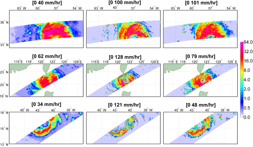
Figure 6: From left to right: TMI-2A12, PR-2A25 and ShARP retrievals. Top to bottom panels: hurricane Danielle in 08/29/2010 (orbit No. 72840) at 09:48 UTC; super typhoon Usagi in 09/21/2013 (orbit No. 90277) at 02:09 UTC; and tropical storm Helene in 09/15/2006 (orbit No. 50338) at 14:34 UTC.

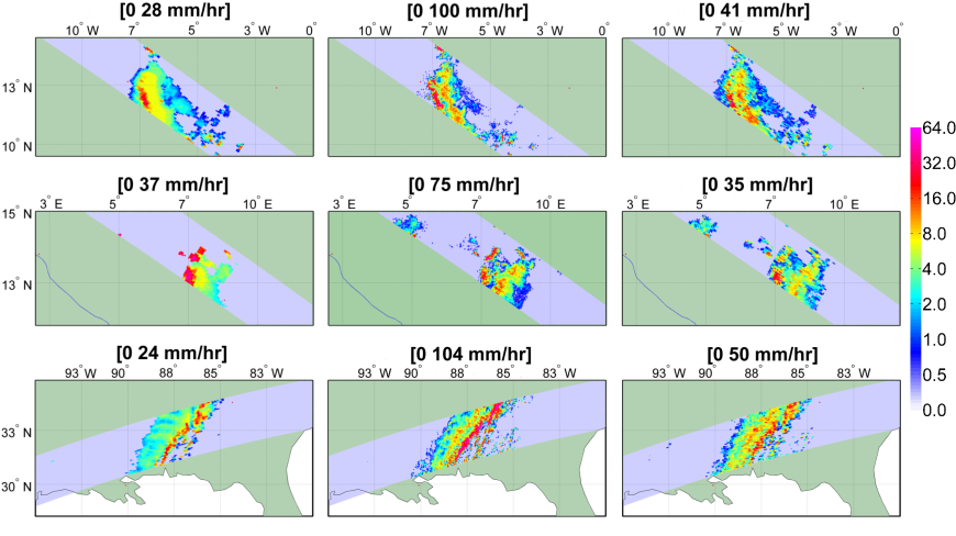
Figure 7: From left to right: TMI-2A12, PR-2A25 and ShARP retrievals. Top-to-bottom panels: a thunderstorm over Mali, Africa in 08/29/2010 (orbit No. 72841) at 10:30 UTC; a summertime thunderstorm over Nigeria, Africa in 06/28/1998 (orbit No. 03357) at 17:43 UTC; and a spring season squall line of precipitation supercells and tornadoes over Georgia, U.S., in 01/30/2013 (orbit No. 86639) at 16:22 UTC.

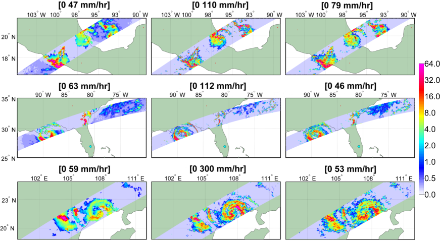
Figure 8: From left to right: TMI-2A12, PR-2A25 and ShARP retrievals. Top to bottom panels: tropical storm Fernand in 08/26/2013 (orbit No. 89874) at 05:30 UTC, hurricane Isaac in 28/08/2012 (orbit No. 84227) at 22:12 UTC and typhoon Kai-tak in 08/17/2012 (orbit No. 84050) at 13:35 UTC.

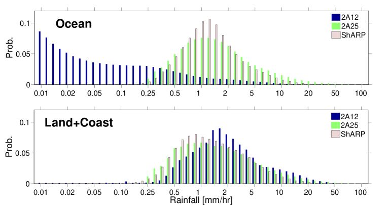
Figure 9: Pixel level probability histograms of the instantaneous rainfall retrievals (> 1e+6 points for each product) for the TMI-2A12 , PR-2A25 and ShARP products over the ocean (top panel) and land-coast (bottom panel) surface classes.

In general, our experiments in Fig. 6, 7, and 8 demonstrate good agreements between the ShARP retrieval and the standard TRMM products. As previously noticed, we typically see that the 2A12 retrieves much larger areas of light rain over ocean compared to the 2A25 and thus to the current implementation of the ShARP algorithm. We see that ShARP can properly recover the storm morphology, high intense and light rainfall both over ocean and land. For example, in the retrieval experiments of the tropical cyclones over ocean (Fig. 6), the high-intensity rainfall cells, curvature and multiband structure of the studied storms are well captured. Over land, in the retrieved thunderstorm over Nigeria (Fig. 6, first row) and the frontal system over Georgia (Fig. 6, bottom row), we see that the ordinary cells and stratiform trailing behind the leading edge of the squall line are well captured. Visual inspections of the retrieved rainfall at the ocean-land interface also confirm that the ShARP retrievals remain coherent over the interface and are in good agreement with the 2A12 and 2A25.

Retrieval Difference Metrics
Metrics	Surface Classes
	Ocean			Land+Coast
	(a)	(b)	(c)	(a)	(b)	(c)
RMSD	5.0	2.8	5.3	6.1	4.3	6.5
MAD	2.3	1.6	2.6	2.7	2.4	3.2
$\rho$	0.55	0.60	0.45	0.50	0.55	0.40

Table 3: Retrieval difference metrics obtained by comparing ShARP vs 2A25 (a), ShARP vs 2A12 (b) and 2A12 vs 2A25 (c) for 100 randomly chosen orbital tracks in 2013. Shown statistics are the Root Mean Squared Difference (RMSD) [mm/hr], Mean Absolute Difference (MAD) [mm/hr] and Spearman’s correlation ($\rho$). The statistics are obtained for instantaneous rainfall estimates at pixel level over the intersection of raining areas of all three retrieval products.

Fig. 9 compares the histogram of the retrieved rainfall values at pixel-level, obtained from 100 randomly sampled orbits of the TRMM in calendar year 2013. Overall, it is seen that the distribution of ShARP and 2A25 are matched well. However, ShARP tends to retrieve more rain around the mode and falls a bit short over the tail. This behavior is somehow expected as ShARP uses a maximum a posteriori estimator that implicitly seeks the mode of the rainfall distribution. As previously noticed, over ocean, 2A12 retrieves much lower rain rates than the other two products. In 2A12, the highest probable range of rainfall intensity falls below 0.02 mm/hr. In effect, more than 75% of raining cases are reported to be below 0.25 mm/hr, while the probability of rainfall at this range is almost zero in the other two products. In 2A25 and ShARP, 63 and 71% of raining cases are within the range of 0.25 to 0.5 mm/hr, respectively, while this probability is around 0.2 in the 2A12. We see that the distribution of the 2A25 over ocean has the thickest tail among the others. In this product, the probability of rainfall exceeding 10 mm/hr is ~5%, while only 1.5% and 0.7% of raining cases are in this range for ShARP and 2A12. Over land and coastal areas, the rainfall distributions of all three products are more or less similar. The mode of the rainfall is around 0.9 mm/hr in ShARP and 2A25, while the highest probable rainfall values are concentrated around 1.9 mm/hr in the 2A12. It is also apparent that the 2A25 and thus ShARP detect more lower rain rates $<1$ mm/hr, while detection of higher rain rates $>10$ mm/hr is more probable in the 2A12 over land. It is important to note that, as the extent of raining areas are different in the studied retrievals, the observed differences in the probability distribution of the instantaneous rainfall do not necessarily lead to large differences in the volumetric retrieved rainfall. In effect, we will show later on that the total annual estimates of rainfall match well in all three products.

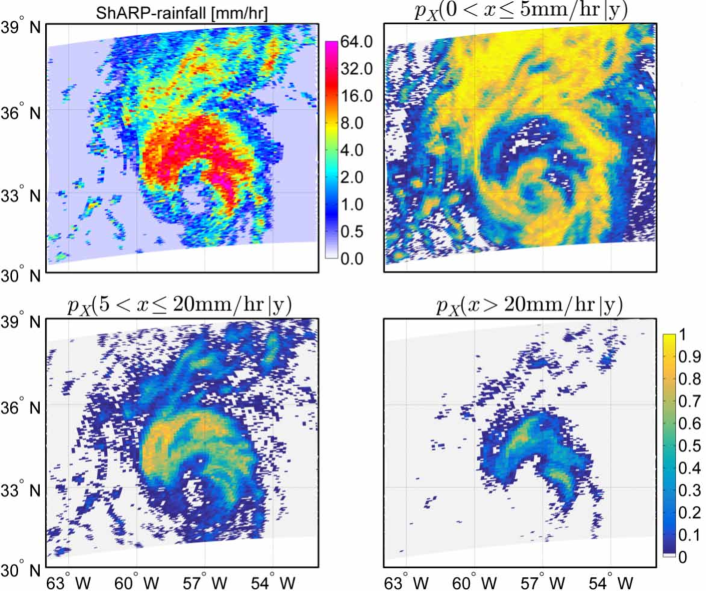
Figure 10: Probability maps showing different segments of the posterior probability density function $p_{X}\left(x|y\right)$ for the ShARP retrieval (top left panel) of the hurricane Danielle (orbit No. 72840) at 09:48 UTC.

Quantiles [mm/hr] of the ShARP Posterior PDF
Bins	Mean	Ocean					Land + Coast
		5th	25th	50th	75th	95th	5th	25th	50th	75th	95th
0.1-0.2	0.15	0.0	0.0	0.0	0.36	1.7	0.0	0.0	0.0	0.0	1.70
0.2-0.5	0.4	0.0	0.0	0.4	0.7	2.2	0.0	0.0	0.3	0.8	2.4
0.5-1.0	0.8	0.0	0.3	0.7	1.2	3.1	0.0	0.4	0.7	1.2	3.4
1.0-2.0	1.5	0.0	0.6	1.1	2.0	5.2	0.0	0.5	1.0	1.9	5.6
2.0-5.0	3.0	0.3	1.0	1.8	3.5	10.0	0.3	0.9	1.8	3.6	10.2
5.0-10.0	7.0	0.7	2.0	4.0	7.9	19.7	0.5	1.6	3.6	7.2	19.6
10.0-25.0	14.0	1.1	3.5	7.4	14.2	35.2	0.7	2.8	6.8	14.7	37.2
25.0-50.0	31.0	2.5	7.7	16.5	31.5	62.5	0.8	5.2	13.8	28.2	68.8

Table 4: Static estimation of key percentiles [mm/hr] of the posterior PDF of the ShARP rainfall retrievals for 100 sampled orbits in calendar year 2013. Second column denotes the mean [mm/hr] values of the retrieved rainfall within each bin.

To further validate the instantaneous retrieval of the ShARP algorithm, we report the Root Mean Squared Difference (RMSD), Mean Absolute Difference (MAD), and the Spearman’s correlation ($\rho$) for each pair of the studied products. Computation of these proximity measures for instantaneous rainfall is not straightforward as these products do not share identical sets of raining areas. Table 3 shows pixel-level estimates of these measures over the intersection of raining areas in the 100 randomly sampled orbits discussed in Fig. 9. As is evident, ShARP and 2A12 are the closest pair while naturally ShARP is closer and more correlated with the 2A25 than that of 2A12. Evaluating the pixel level differences of the rainfall samples, among the studied products, shows that typically a large number of those deviations are very small while a small number of them are typically very large. For instance, more than 55% of the differences between ShARP and 2A25 are less than 1 mm/hr while less than 5% of them are greater than 8 mm/hr. This can be the main reason why the RMSD is almost twice that of the MAD metric in Table 3. In effect, the RMSD can be easily saturated by a few large deviations as it quadratically penalizes them. On the other hand, MAD linearly penalizes the differences and seems to be a more robust measure against a few number of large deviations.

As we explained, the posterior density of the ShARP retrievals can be empirically approximated via counting the frequency of rainfall occurrence in the atoms of the rainfall sub-dictionaries. Table 4 reports a static estimation of key percentiles of the posterior PDF for the examined 100 orbits. For brevity, we only present the results for the rainfall values falling between 0.1, 0.2, 0.5, 1, 2, 5, 10, 25 and 50 mm/hr. Fig. 10 also shows some dynamic probability maps of the posteriori PDF for the snapshot of the hurricane Danielle shown in the Fig. 6. Clearly, this important feature of ShARP allows us to perform rainfall retrieval probabilistically and track the high risk areas of the extreme rainfall based on a certain probability of exceedance.

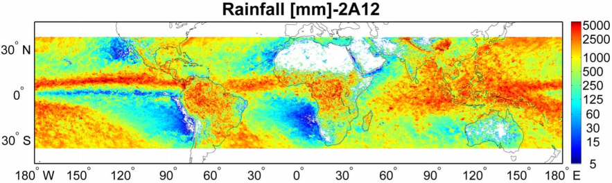
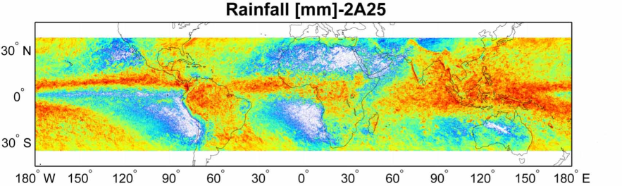
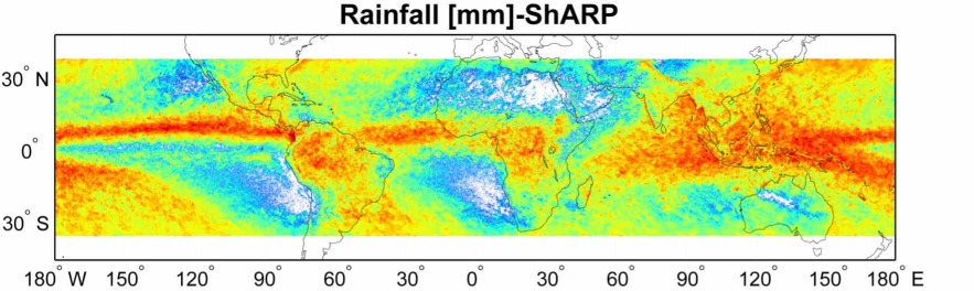
Figure 11: Annual estimates of the total rainfall [mm] in 2013 mapped onto a 0.1-degree grid box. From top to bottom panels: 2A12, 2A25, and ShARP retrieval products.

4.3 Cumulative Experiments

To validate the results of our algorithm in a cumulative sense, we focus on all orbital observations of the TRMM in calendar year 2013. To unify the sampling rate, we only use the available observations over the inner swath, where both sensors provide overlapping and validated rainfall observations. Fig. 11 demonstrates the annual rainfall estimates, mapped onto a $0.1^{\circ}\times 0.1^{\circ}$ grid. In general, we see a good agreement between ShARP and the standard TRMM products. Here, as the 2A25 potentially provides one of the best spaceborne estimates of the total rainfall volume over the tropics [see, 5], we also study deviations of the passive retrievals from this active product.

At $0.1$-degree resolution, the normalized root mean squared difference ($\text{RMSD}_{\text{n}}$) is about 36% and 48% for ShARP (Fig. 11, bottom panel) and 2A12 (Fig. 11, top panel), respectively. At the coarser resolution of $1^{\circ}\times 1^{\circ}$ grid box, this metric reduces to 17% and 31% (Fig. 12), while the overall correlation with 2A25 is 0.92 and 0.97 for the 2A12 and ShARP (Fig. 13). Zonal mean values are also demonstrated in Fig. 14 with quantitative explanations in Table 5. Over ocean, except in the North Atlantic mid-latitude storm tracks, both ShARP and 2A12 slightly overestimate the total rainfall obtained from 2A25, while most of the underestimation regions are spread over land, especially near coastal zones, islands and peninsulas, although some overestimation can be seen in the Central Africa and South America in both 2A12 and ShARP.

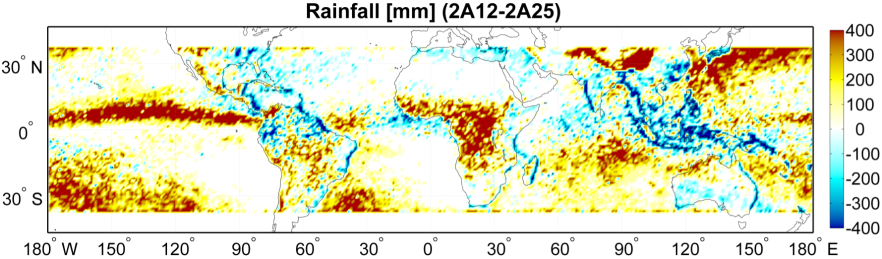
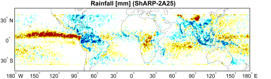
Figure 12: Annual estimates of the total rainfall difference [mm] for calendar year 2013. From top to bottom panels: The difference between the 2A12, and ShARP retrievals with the 2A25 at grid size $1^{\circ}\times 1^{\circ}$. Hot (red) and cold (blue) colors denote intensity of positive and negative differences.

Fig. 12 shows that passive retrieval products overestimate (~ 300-400 mm) 2A25 on the narrow ridge of high precipitation in the Intertropical Convergence Zone (ITCZ) across the Pacific Ocean. As is evident, over the South Pacific, Atlantic, and Indian Ocean convergence zones, we also see some over estimation in ShARP, while the positive difference is relatively mitigated compared to the standard 2A12. In the North Atlantic mid-latitude storm tracks, both passive retrievals slightly underestimate the annual rainfall while the deviations are smaller in the 2A12 compared to ShARP.

Some promising results of our algorithm seem to be over land and coastal zones. Over the subtropical hot desert, arid and semi-arid climates (e.g., Sahara, Arabian, Syrian deserts, and central Iran plateau), we see that ShARP retrieves well the low rainfall amounts seen by the PR. Over the Central Africa, both 2A12 and ShARP overestimate the 2A25 annual rainfall while the gap seems to be smaller in ShARP. Over the North America, it is seen that 2A12 shows good agreement with the PR estimates over the East Coast and Midwest of the United States. However, ShARP approximates well the PR over the West Coast and Southwest where the rainfall signatures are predominantly corrupted with noise due to the highly emissive desert surfaces. Over South America, ShARP shows improved retrieval over Brazil and southern Amazon, while, compared to the 2A12, notable underestimation can be seen over the northern Amazon basin, Colombia and Venezuela. Some improved results of our algorithm are over the snow-covered Tibetan highlands and Himalayas. We can see that ShARP can distinguish well the background noise from rainfall signatures and reduces some overestimation seen in the 2A12. Note that, we have used minimal number of the earth surface classifications and have not defined any specific class over the Tibetan Plateau. Indeed, due to the 9-dimensional nearest neighborhood selection of the spectral sub-dictionaries, our algorithm is apparently capable to robustly eliminate a large portion of the physically inconsistent spectral candidates in the detection step. Over Southeast Asia, where the rainfall signatures are masked by a mixture of ocean and land surface background radiation regimes, both ShARP and 2A12 underestimate the 2A25. However, the negative differences in ShARP are slightly reduced, compared to the 2A12, especially over Indonesia, Malaysia and Philippines.

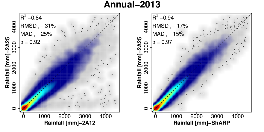
Figure 13: Smooth scatter plots of the annual retrieved rainfall [mm] by the 2A12 (left panel) and ShARP (right panel) versus the 2A25 at grid size $1^{\circ}\times 1^{\circ}.$ Hot (red) and cold (blue) colors denote higher and lower density of the available rainfall intensity pairs. The R-square denotes the coefficient of determination, $\text{RMSD}_{\text{n}}$ and $\text{MAD}_{\text{n}}$ are the normalized root mean squared and mean absolute difference while $\rho$ denotes the correlation coefficient.

Comparison of the total annual zonal mean values (Fig. 14, left panel) shows that ShARP approximates well the average latitudinal rainfall distribution and budget. We can see that not only over the tropics but also over the mid-latitudes, where stratiform rainfall is dominant, ShARP well reconstructs the 2A25 product over ocean (Fig. 14, middle panel). Over land, ShARP underestimates the zonal mean within a narrow band (latitudes $5{}^{\circ}$S-N) around the tropics, while it performs well over the subtropical climate zones (Fig. 14, right panel). This underestimation is contributed mainly by the ShARP poor retrieval skill over the northern part of the South America. Quantitative comparison of these zonal profiles is presented in Table 5.

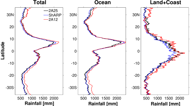
Figure 14: Annual rainfall zonal mean values [mm] obtained from estimates of the annual rainfall shown in Fig. 11. From left to right panels: zonal mean values computed over all surface classes, over ocean and over land-coasts.

Product	Surface Class	Annual Zonal Mean
		RMSD	MD
ShARP-2A25	Total	40.20	-6.53
	Ocean	47.61	7.15
	Land + Coast	95.67	-41.02
2A12-2A25	Total	103.04	73.63
	Ocean	99.50	69.42
	Land + Coast	137.62	79.43

Table 5: Retrieval skills including RMSD [mm] and mean difference (MD) [mm] for the annual zonal mean values shown in Fig. 14.

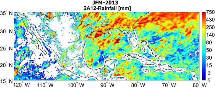
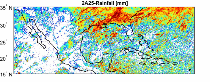
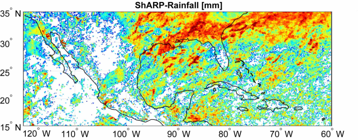
Figure 15: Inter-annual rainfall accumulation for the period from January through March (JFM) in 2013, mapped onto a 0.1-degree grid box.

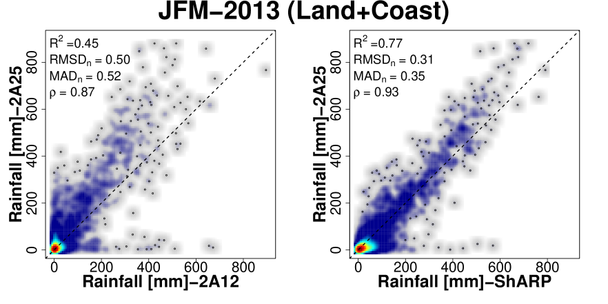
Figure 16: Smooth scatter plots of the 3-month rainfall accumulation [mm], shown in Fig. 15. The plots show the 2A12 (left panel) and ShARP (right panel) versus the 2A25 at $0.5\times 0.5^{\circ}$ grid box. See caption of Fig. 13 for explanations of the presented statistics.

To briefly evaluate inter-annual performance of our algorithm, especially over land and coastal areas, we also focused on a 3-month rainfall accumulation for the period from January through March (JFM) of 2013. We confined the spatial extent of our evaluation within latitudes $15$-$35{}^{\circ}$N and longitudes $60$-$120{}^{\circ}$W (Fig. 15). The storm system of the area in the JFM period is mainly supplied by the moisture coming from the Pacific Ocean through the subtropical jet stream and is intensified where the extratropical lifting saturates the atmospheric column over the Gulf of Mexico. This mechanism typically causes heavy precipitation events over the southeast of the United States and the Gulf of Mexico, while it leaves the southwest relatively dry. Overall, we see that ShARP properly retrieves the high and low seasonal precipitation amounts in the JFM system and its retrieved rainfall resembles well the standard TRMM products. Specifically, it is seen that in the vicinity of coast lines of the Caribbean Islands and Bahamas, the light rainfall values are well captured by ShARP. During this period, consistent with the instantaneous results shown in Fig. 5, the largest amount of raining areas over the ocean is detected by the 2A12 (88% of ocean), while this fraction is 71 and 66% in the ShARP and 2A25. In contrast, ShARP detects the largest raining area (69%) over land, while this fraction is 63 and 50% in the 2A25 and 2A12 . The main factor contributing to the overestimation of the 2A25 by ShARP is primarily due to the coarse resolution of the TMI sensor which is unable to resolve signatures of small-scale precipitation events captured by the PR. A brief quantitative comparison of the JFM rainfall system, only over land and coastal areas, is presented in Fig. 16. As is evident, ShARP well correlates with the 2A25, while we see some discrepancies showing that for some light raining areas in the 2A25, both ShAPR and 2A12 retrieve high rainfall values. It turns out that some of these anomalies are due, in part, to miss interpretation of the highly emissive ground as rainfall signatures. For example, we see that over the Baja California Desert, ShARP exhibits over estimation spots while snow-covered land surface in the month of January confuses the 2A12 algorithm over the north west of Arizona (~$110{}^{\circ}$W, $35^{\circ}$N).

5 CONCLUDING REMARKS

We proposed a Bayesian microwave rainfall retrieval algorithm that makes use of a priori collected rainfall and spectral dictionaries. This algorithm relies on a nearest neighborhood detection rule and exploits modern shrinkage estimation paradigms. We have examined its performance using empirical dictionaries populated from coincidental observations of the TRMM precipitation radar (PR) and Microwave Imager (TMI) and demonstrated its considerable promise to provide accurate rainfall retrievals especially over land and coastal areas. In future research, the algorithm needs to be further verified for different rainfall regimes over ocean and land. Further efforts also need to be devoted for improving the retrieval of rainfall extremes both over land and ocean. While we have confined our experiments to empirical dictionaries, the core of our algorithm is flexible and versatile enough to exploit both observational and physically-based generated dictionaries. The proposed implementation is very parsimonious at this stage and further refinements, such as smarter choices of surface classes by considering ground emissivity patterns and adding auxiliary state variables to the dictionaries (e.g., surface skin temperature, total column water) can definitely improve performance of the proposed approach. Currently, we are developing a new version of this algorithm that uses compact dictionaries for faster and more accurate retrieval of the entire rainfall profile. The particular emphasis will be on the available spectral bands (10.65 to 183 GHz) of the radiometer and observations of the dual frequency precipitation radar aboard the successfully launched Global Precipitation Measuring (GPM) satellites.

References

- Arkin [1979] Arkin, P. A. (1979), The Relationship between Fractional Coverage of High Cloud and Rainfall Accumulations during GATE over the B-Scale Array, Mon. Wea. Rev., 107(10), 1382–1387, doi:10.1175/1520-0493(1979)107<1382:TRBFCO>2.0.CO;2.
- Arkin and Ardanuy [1989] Arkin, P. A., and P. E. Ardanuy (1989), Estimating Climatic-Scale Precipitation from Space: A Review, J. Climate, 2(11), 1229–1238, doi:10.1175/1520-0442(1989)002<1229:ECSPFS>2.0.CO;2.
- Barrett [1970] Barrett (1970), The Estimatipo of Monthly Rainfall from Satellite, Mon. Wea. Rev., 98(4), 322–327, doi:10.1175/1520-0493(1970)098<0322:TEOMRF>2.3.CO;2.
- Berg et al. [2006] Berg, W., T. L’Ecuyer, and C. Kummerow (2006), Rainfall climate regimes: The relationship of regional trmm rainfall biases to the environment, J. Appl. Meteor. Climatol., 45(3), 434–454, doi:10.1175/JAM2331.1.
- Berg et al. [2009] Berg, W., T. L’Ecuyer, and J. M. Haynes (2009), The distribution of rainfall over oceans from spaceborne radars, J. Appl. Meteor. Climatol., 49(3), 535–543, doi:10.1175/2009JAMC2330.1.
- Blackmer [1975] Blackmer, R. H. (1975), Correlation of Cloud Brightness and Radiance with Precipitation Intensity., Tech. rep., Stanford Res. Inst. Menlo Park, CA. Final Report–Task B (NEPRF TR8–75 (SRI)).
- Boyd and Vandenberghe [2004] Boyd, S., and L. Vandenberghe (2004), Convex optimization, 716 pp., Cambridge University Press, New York.
- Chen et al. [1998] Chen, S. S., D. L. Donoho, and M. A. Saunders (1998), Atomic decomposition by basis pursuit, SIAM J. Sci. Comput., 20, 33–61.
- Donoho [1995] Donoho, D. (1995), De-noising by soft-thresholding, IEEE Trans. Inform. Theory., 41(3), 613–627, doi:10.1109/18.382009.
- Ebtehaj et al. [2012] Ebtehaj, A. M., E. Foufoula-Georgiou, and G. Lerman (2012), Sparse regularization for precipitation downscaling, J. Geophys. Res., 116, D22110, doi:10.1029/2011JD017057.
- Elad [2010] Elad, M. (2010), Sparse and Redundant Representations: From Theory to Applications in Signal and Image Processing, 376 pp., Springer Verlag, New York, NY.
- Ellis et al. [2009] Ellis, T. D., T. L’Ecuyer, J. M. Haynes, and G. L. Stephens (2009), How often does it rain over the global oceans? The perspective from CloudSat, Geophys. Res. Lett., 36(3), doi:10.1029/2008GL036728.
- Evans et al. [1995] Evans, K. F., J. Turk, T. Wong, and G. L. Stephens (1995), A Bayesian Approach to Microwave Precipitation Profile Retrieval, J. Appl. Meteor., 34(1), 260–279, doi:10.1175/1520-0450-34.1.260.
- Ferraro et al. [1994] Ferraro, R. R., N. C. Grody, and G. F. Marks (1994), Effects of surface conditions on rain identification using the dmsp-ssm/i, Remote Sens. Rev., 11(1-4), 195–209, doi:10.1080/02757259409532265.
- Ferraro et al. [1998a] Ferraro, R. R., E. A. Smith, W. Berg, and G. J. Huffman (1998a), A Screening Methodology for Passive Microwave Precipitation Retrieval Algorithms, J. Atmos. Sci., 55(9), 1583–1600, doi:10.1175/1520-0469(1998)055<1583:ASMFPM>2.0.CO;2.
- Ferraro et al. [1998b] Ferraro, R. R., E. A. Smith, W. Berg, and G. J. Huffman (1998b), A screening methodology for passive microwave precipitation retrieval algorithms, J. Atmos. Sci., 55(9), 1583–1600, doi:10.1175/1520-0469(1998)055<1583:ASMFPM>2.0.CO;2.
- Foufoula-Georgiou et al. [2014] Foufoula-Georgiou, E., A. Ebtehaj, S. Zhang, and A. Hou (2014), Downscaling Satellite Precipitation with Emphasis on Extremes: A Variational -Nrom Regularization in the Derivative Domain, Surveys in Geophysics, pp. 1–19, doi:10.1007/s10712-013-9264-9.
- Grecu and Anagnostou [2002] Grecu, M., and E. N. Anagnostou (2002), Use of Passive Microwave Observations in a Radar Rainfall-Profiling Algorithm, J. Appl. Meteor., 41(7), 702–715, doi:10.1175/1520-0450(2002)041<0702:UOPMOI>2.0.CO;2.
- Grecu and Olson [2006] Grecu, M., and W. S. Olson (2006), Bayesian Estimation of Precipitation from Satellite Passive Microwave Observations Using Combined Radar-Radiometer Retrievals, J. Appl. Meteor. Climatol., 45(3), 416–433, doi:10.1175/JAM2360.1.
- Grecu et al. [2004] Grecu, M., W. S. Olson, and E. N. Anagnostou (2004), Retrieval of Precipitation Profiles from Multiresolution, Multifrequency Active and Passive Microwave Observations, J. Appl. Meteor., 43(4), 562–575, doi:10.1175/1520-0450(2004)043<0562:ROPPFM>2.0.CO;2.
- Grody [1991] Grody, N. C. (1991), Classification of snow cover and precipitation using the special sensor microwave imager, J. Geophys. Res., 96(D4), 7423–7435, doi:10.1029/91JD00045.
- Haddad et al. [1997] Haddad, Z., E. Smith, C. Kummerow, T. Iguchi, M. Farrar, S. Durden, M. Alves, and W. Olson (1997), The TRMM ’day-1’ radar/radiometer combined rain-profiling algorithm, J. Meteor. Soc. Japan, 75(4), 799–809.
- Hansen [2010] Hansen, P. (2010), Discrete inverse problems: insight and algorithms, vol. 7, Society for Industrial & Applied Mathematics (SIAM), Philadelphia, PA, USA.
- Hsu et al. [1997] Hsu, K., X. Gao, S. Sorooshian, and H. Gupta (1997), Precipitation estimation from remotely sensed information using artificial neural networks, J. Appl. Meteorol., 36(9), 1176–1190.
- Iguchi et al. [2000] Iguchi, T., T. Kozu, R. Meneghini, J. Awaka, and K. i. Okamoto (2000), Rain-Profiling Algorithm for the TRMM Precipitation Radar, J. Appl. Meteor., 39(12), 2038–2052, doi:10.1175/1520-0450(2001)040<2038:RPAFTT>2.0.CO;2.
- Janssen [1993] Janssen, M. A. (1993), Atmospheric remote sensing by microwave radiometry, John Wiley & Sons, Inc., New York, NY.
- Kilonsky and Ramage [1976] Kilonsky, B. J., and C. S. Ramage (1976), A Technique for Estimating Tropical Open-Ocean Rainfall from Satellite Observations, J. Appl. Meteor., 15(9), 972–975, doi:10.1175/1520-0450(1976)015<0972:ATFETO>2.0.CO;2.
- Kummerow and Giglio [1994] Kummerow, C., and L. Giglio (1994), A Passive Microwave Technique for Estimating Rainfall and Vertical Structure Information from Space. Part I: Algorithm Description, J. Appl. Meteor., 33(1), 3–18, doi:10.1175/1520-0450(1994)033<0003:APMTFE>2.0.CO;2.
- Kummerow et al. [1996] Kummerow, C., W. S. Olson, and L. Giglio (1996), A simplified scheme for obtaining precipitation and vertical hydrometeor profiles from passive microwave sensors, IEEE Trans. Geosci. Remote., 34(5), 1213–1232, doi:10.1109/36.536538.
- Kummerow et al. [1998] Kummerow, C., W. Barnes, T. Kozu, J. Shiue, and J. Simpson (1998), The Tropical Rainfall Measuring Mission (TRMM) Sensor Package, J. Atmos. Oceanic Technol., 15(3), 809–817, doi:10.1175/1520-0426(1998)015<0809:TTRMMT>2.0.CO;2.
- Kummerow et al. [2001] Kummerow, C., Y. Hong, W. Olson, S. Yang, R. Adler, J. McCollum, R. Ferraro, G. Petty, D. Shin, and T. Wilheit (2001), The evolution of the Goddard Profiling Algorithm (GPROF) for rainfall estimation from passive microwave sensors, J. Appl. Meteorol., 40(11), 1801–1820.
- Kummerow et al. [2011] Kummerow, C. D., S. Ringerud, J. Crook, D. Randel, and W. Berg (2011), An Observationally Generated A Priori Database for Microwave Rainfall Retrievals, J. Atmos. Oceanic Technol., 28(2), 113–130, doi:10.1175/2010JTECHA1468.1.
- Lécuyer and Stephens [2002] Lécuyer, T. S., and G. L. Stephens (2002), An uncertainty model for bayesian monte carlo retrieval algorithms: Application to the trmm observing system, Quarterly Journal of the Royal Meteorological Society, 128(583), 1713–1737, doi:10.1002/qj.200212858316.
- Li et al. [1996] Li, Q., R. L. Bras, and D. Veneziano (1996), Passive microwave remote sensing of rainfall considering the effects of wind and nonprecipitating clouds, J. Geophys. Res., 101(D21), 26,503–26,515, doi:10.1029/96JD01388.
- Liu and Curry [1992] Liu, G., and J. A. Curry (1992), Retrieval of precipitation from satellite microwave measurement using both emission and scattering, Journal of Geophysical Research: Atmospheres, 97(D9), 9959–9974, doi:10.1029/92JD00289.
- Lovejoy and Austin [1979] Lovejoy, S., and G. Austin (1979), The delineation of rain areas from visible and IR satellite data for GATE and mid–latitudes, Atmosphere-Ocean, 17(1), 77–92, doi:10.1080/07055900.1979.9649053.
- Marzano et al. [1999] Marzano, F., A. Mugnai, G. Panegrossi, N. Pierdicca, E. Smith, and J. Turk (1999), Bayesian estimation of precipitating cloud parameters from combined measurements of spaceborne microwave radiometer and radar, Geoscience and Remote Sensing, IEEE Transactions on, 37(1), 596–613, doi:10.1109/36.739124.
- McCollum and Ferraro [2005] McCollum, J. R., and R. R. Ferraro (2005), Microwave rainfall estimation over coasts, J. Atmos. Oceanic Technol., 22(5), 497–512, doi:10.1175/JTECH1732.1.
- Mehrotra [1992] Mehrotra, S. (1992), On the Implementation of a Primal-Dual Interior Point Method, SIAM J. Optim., 2, 575–601.
- Mugnai et al. [1993] Mugnai, A., E. A. Smith, and G. J. Tripoli (1993), Foundations for statisticalphysical precipitation retrieval from passive microwave satellite measurements. part ii: Emission-source and generalized weighting-function properties of a time-dependent cloud-radiation model, J. Appl. Meteor., 32(1), 17–39, doi:10.1175/1520-0450(1993)032<0017:FFSPRF>2.0.CO;2.
- Olson [1989] Olson, W. S. (1989), Physical retrieval of rainfall rates over the ocean by multispectral microwave radiometry: Application to tropical cyclones, J. Geophys. Res., 94(D2), 2267–2280, doi:10.1029/JD094iD02p02267.
- Olson et al. [1996] Olson, W. S., C. D. Kummerow, G. M. Heymsfield, and L. Giglio (1996), A method for combined passive-active microwave retrievals of cloud and precipitation profiles, J. Appl. Meteor., 35(10), 1763–1789, doi:10.1175/1520-0450(1996)035<1763:AMFCPM>2.0.CO;2.
- Petty [1994a] Petty, G. (1994a), Physical retrievals of over-ocean rain rate from multichannel microwave imagery. part i: Theoretical characteristics of normalized polarization and scattering indices, Meteorology and Atmospheric Physics, 54(1-4), 79–99, doi:10.1007/BF01030053.
- Petty [1994b] Petty, G. (1994b), Physical retrievals of over-ocean rain rate from multichannel microwave imagery. part ii: Algorithm implementation, Meteorology and Atmospheric Physics, 54(1-4), 101–121, doi:10.1007/BF01030054.
- Petty [1994c] Petty, G. (1994c), Physical retrievals of over-ocean rain rate from multichannel microwave imagery. part i: Theoretical characteristics of normalized polarization and scattering indices, Meteor. Atmos. Phys., 54(1-4), 79–99, doi:10.1007/BF01030053.
- Petty and Katsaros [1990] Petty, G. W., and K. B. Katsaros (1990), Precipitation observed over the south china sea by the nimbus-7 scanning multichannel microwave radiometer during winter monex, J. Appl. Meteor., 29(4), 273–287, doi:10.1175/1520-0450(1990)029<0273:POOTSC>2.0.CO;2.
- Petty and Krajewski [1996] Petty, G. W., and W. F. Krajewski (1996), Satellite estimation of precipitation over land, Hydrological Sciences Journal, 41(4), 433–451, doi:10.1080/02626669609491519.
- Petty and Li [2013a] Petty, G. W., and K. Li (2013a), Improved Passive Microwave Retrievals of Rain Rate Over Land and Ocean. 1. Algorithm description, J. Atmos. Oceanic Technol., doi:10.1175/JTECH-D-12-00144.1.
- Petty and Li [2013b] Petty, G. W., and K. Li (2013b), Improved Passive Microwave Retrievals of Rain Rate Over Land and Ocean. 2. Validation and Intercomparison, J. Atmos. Oceanic Technol., doi:10.1175/JTECH-D-12-00184.1.
- Roweis and Saul [2000] Roweis, S. T., and L. K. Saul (2000), Nonlinear Dimensionality Reduction by Locally Linear Embedding, Science, 290(5500), 2323–2326, doi:10.1126/science.290.5500.2323.
- Seto et al. [2005] Seto, S., N. Takahashi, and T. Iguchi (2005), Rain/No-Rain Classification Methods for Microwave Radiometer Observations over Land Using Statistical Information for Brightness Temperatures under No-Rain Conditions, J. Appl. Meteor., 44(8), 1243–1259, doi:10.1175/JAM2263.1.
- Sharkov [2003] Sharkov, E. A. (2003), Passive Microwave Remote Sensing of the Earth: Physical Foundations, 613 pp., Praxis Publishing, Springer, Chichester, UK.
- Skofronick-Jackson et al. [2003] Skofronick-Jackson, G. M., J. R. Wang, G. M. Heymsfield, R. Hood, W. Manning, R. Meneghini, and J. A. Weinman (2003), Combined radiometer-radar microphysical profile estimations with emphasis on high-frequency brightness temperature observations, J. Appl. Meteor., 42(4), 476–487, doi:10.1175/1520-0450(2003)042<0476:CRRMPE>2.0.CO;2.
- Spencer [1986] Spencer, R. W. (1986), A satellite passive 37-ghz scattering-based method for measuring oceanic rain rates, J. Climate Appl. Meteor., 25(6), 754–766, doi:10.1175/1520-0450(1986)025<0754:ASPGSB>2.0.CO;2.
- Spencer et al. [1983] Spencer, R. W., D. W. Martin, B. B. Hinton, and J. A. Weinman (1983), Satellite microwave radiances correlated with radar rain rates over land, Nature, 304, 141–143.
- Tibshirani [1996] Tibshirani, R. (1996), Regression Shrinkage and Selection via the Lasso, J. R. Stat. Soc. Ser. B Stat. Methodol., 58(1), 267–288.
- Tikhonov et al. [1977] Tikhonov, A., V. Arsenin, and F. John (1977), Solutions of ill-posed problems, Winston & Sons. Washington, DC.
- Wilheit [1979] Wilheit, T. (1979), A model for the microwave emissivity of the ocean’s surface as a function of wind speed, Geoscience Electronics, IEEE Transactions on, 17(4), 244–249, doi:10.1109/TGE.1979.294653.
- Wilheit et al. [1994] Wilheit, T., R. Adler, S. Avery, E. Barrett, P. Bauer, W. Berg, A. Chang, J. Ferriday, N. Grody, S. Goodman, C. Kidd, D. Kniveton, C. Kummerow, A. Mugnai, W. Olson, G. Petty, A. Shibata, and E. Smith (1994), Algorithms for the retrieval of rainfall from passive microwave measurements, Remote Sens. Rev., 11(1-4), 163–194, doi:10.1080/02757259409532264.
- Wilheit et al. [2003] Wilheit, T., C. Kummerow, and R. Ferraro (2003), Rainfall algorithms for AMSR-E, IEEE Trans. Geosci. Remote Sens., 41(2), 204–214, doi:10.1109/TGRS.2002.808312.
- Wilheit et al. [1977] Wilheit, T. T., A. T. C. Chang, M. S. V. Rao, E. B. Rodgers, and J. S. Theon (1977), A Satellite Technique for Quantitatively Mapping Rainfall Rates over the Oceans, J. Appl. Meteor., 16(5), 551–560, doi:10.1175/1520-0450(1977)016<0551:ASTFQM>2.0.CO;2.
- Zhang [1995] Zhang, Y. (1995), Solving Large-Scale Linear Programs by Interior-Point Methods Under the MATLAB Environment, Tech. rep., Department of Mathematics and Statistics, University of Maryland, Baltimore County, Baltimore, MD, Technical Report TR96-01, July.
- Zhou et al. [2006] Zhou, Y., D. McLaughlin, and D. Entekhabi (2006), Assessing the performance of the ensemble Kalman filter for land surface data assimilation, Mon. Weather Rev., 134(8), 2128–2142.
- Zou and Hastie [2005] Zou, H., and T. Hastie (2005), Regularization and variable selection via the elastic net, J. R. Stat. Soc. Ser. B Stat. Methodol., 67(2), 301–320, doi:10.1111/j.1467-9868.2005.00503.x.