Border Bases for Polynomial Rings over Noetherian Rings

Abstract.

The theory of border bases for zero-dimensional ideals has attracted several researchers in symbolic computation due to their numerical stability and mathematical elegance. As shown in (Francis & Dukkipati, J. Symb. Comp., 2014), one can extend the concept of border bases over Noetherian rings whenever the corresponding residue class ring is finitely generated and free. In this paper we address the following problem: Can the concept of border basis over Noetherian rings exists for ideals when the corresponding residue class rings are finitely generated but need not necessarily be free modules? We present a border division algorithm and prove the termination of the algorithm for a special class of border bases. We show the existence of such border bases over Noetherian rings and present some characterizations in this regard. We also show that certain reduced Gröbner bases over Noetherian rings are contained in this class of border bases.

1. Introduction

Gröbner bases theory for polynomial rings over fields gives an algorithmic technique to determine a vector space basis of the residue class ring modulo a zero dimensional ideal (Buchberger, 1965). The theory of Gröbner bases was extended to polynomial rings over Noetherian commutative rings with unity a few decades ago (e.g. Trinks, 1978; Möller, 1988; Zacharias, 1978). For a good exposition on Gröbner bases over rings one can refer to (Adams & Loustaunau, 1994).

Certain recent developments in cryptography and other fields have led to renewed interest in polynomial rings over rings (Greuel et al., 2011). For instance, free residue class rings over $\mathbb{Z}[x]$ called ideal lattices (Lyubashevsky & Micciancio, 2006) have been shown to be isomorphic to integer lattices, an important cryptographic primitive (Ajtai, 1996) and certain cyclic lattices in $\mathbb{Z}[x]$ have been used in NTRU cryptographic schemes (Hoffstein et al., 1998). Boolean polynomial rings over a boolean ring is another important example of a polynomial ring over a ring since it can be used to solve combinatorial puzzles like Sudoku (Sato et al., 2011). Another example is the polynomial rings over $\mathbb{Z}/2^{k}$. They are used to prove the correctness of data paths in system-on-chip design (Greuel et al., 2011).

Border bases, an alternative to Gröbner bases, are well studied for polynomial rings over fields (Kehrein et al., 2005; Kehrein & Kreuzer, 2005). Though border bases are restricted to zero dimensional ideals, the motivation for border bases comes from the numerical stability of border bases over Gröbner bases (Stetter, 2004). There has been considerable interest in the theory of border bases, from characterization (Kehrein & Kreuzer, 2005) to methods of computation (Kehrein & Kreuzer, 2006) to computational hardness (Ananth & Dukkipati, 2012). The concept of border bases can be easily extended to polynomial rings over rings if the corresponding residue class ring has a free $A$-module representation w.r.t. some monomial order and is finitely generated as an $A$-module (Francis & Dukkipati, 2014). In this paper, we study border bases for ideals in polynomial rings over Noetherian commutative rings in a more general set up.

2. Background & Preliminaries

2.1. Notations

A polynomial ring in indeterminates $x_{1},\ldots,x_{n}$ over a Noetherian, commutative ring $A$ is denoted by $A[x_{1},\ldots,x_{n}]$. Throughout this paper, the rings we study are rings with unity. The set of all ideals of $A$ is denoted by $\operatorname{Id}(A)$. When $A=\Bbbk$, where $\Bbbk$ is a field, we write it as $\Bbbk[x_{1},\ldots,x_{n}]$. A monomial in indeterminates $x_{1},\ldots,x_{n}$ is denoted by $x^{\alpha}$, where $\alpha\in\mathbb{N}^{n}$, and the set of all monomials is denoted by $\mathbb{M}^{n}$. By ‘term’ we mean $cx^{\alpha}$, where $c\in A$ and $c\neq 0$. We will denote all the terms in $A[x_{1},\ldots,x_{n}]$ by $\mathbb{T}^{n}$. Let $T\subseteq\mathbb{T}^{n}$ be a set of terms, possibly infinite. We define the monomial part of $T$, denoted by $\operatorname{Mon}(T)$, as $\operatorname{Mon}(T)=\{x^{\alpha}\in\mathbb{M}^{n}:ax^{\alpha}\in T,\text{ for some nonzero }a\in A\}$.

A polynomial $f$ is denoted by $f=\sum_{\alpha\in\Lambda}a_{\alpha}x^{\alpha}$, where $a_{\alpha}\in A$, $\alpha\in\mathbb{N}^{n}$ and $\Lambda\subseteq{\mathbb{N}}^{n}$ is a finite set. $\Lambda$ is called the support of the polynomial $f$, denoted by $\operatorname{supp}(f)$. The set of monomials appearing with nonzero coefficients in $f$ is denoted by $\operatorname{Mon}(f)$. The set of all terms appearing in $f$ is denoted by $\operatorname{Ter}(f)$, i.e. $\operatorname{Ter}(f)=\{a_{\alpha}x^{\alpha}\mid\alpha\in\Lambda\}$. If $F$ is a set of polynomials then $\operatorname{Mon}(F)=\bigcup_{f\in F}\operatorname{Mon}(f)$. Similarly, $\operatorname{Ter}(F)=\bigcup_{f\in F}\operatorname{Ter}(f)$. Given a set of terms $T$ and an ideal $\mathfrak{a}$ in $A[x_{1},\ldots,x_{n}]$, the set of residue class elements of $T$ modulo $\mathfrak{a}$ is denoted by $T+\mathfrak{a}$. That is $T+\mathfrak{a}=\{ax^{\alpha}+\mathfrak{a}:ax^{\alpha}\in T\}$. Given a set of polynomials $F$ the span of $F$ over $A$ is given by $\operatorname{Span}_{A}(F)=\{\sum_{i=1}^{s}a_{i}f_{i}:a_{i}\in A,f_{i}\in F,s\in\mathbb{N}\}$.

With respect to a monomial order $\prec$, the leading monomial, leading coefficient and leading term of a polynomial $f\in A[x_{1},\ldots,x_{n}]$ are denoted by $\operatorname{Lm}(f)$, $\operatorname{Lc}(f)$ and $\operatorname{Lt}(f)$ respectively. That is, we have $\operatorname{Lt}(f)=\operatorname{Lc}(f)\operatorname{Lm}(f)$. Given a set of polynomials $S$, possibly infinite, $\operatorname{Lt}(S)$ denotes the set of all leading terms of polynomials in $S$. The leading term ideal (or initial ideal) of $S$ is denoted by $\langle\operatorname{Lt}(S)\rangle$ and is given by $\langle\operatorname{Lt}(S)\rangle=\langle\{\mathrm{Lt}_{\prec}(f)\mid f\in S\}\rangle$. Similarly, the leading monomial ideal and the leading coefficient ideal of $S$ are denoted by $\langle\operatorname{Lm}(S)\rangle$ and $\langle\operatorname{Lc}(S)\rangle$ respectively. Note that the leading coefficient ideal is an ideal in the coefficient ring, $A$. The ideal generated by the polynomials $f_{1},\ldots,f_{s}$ is denoted by $\langle f_{1},\ldots,f_{s}\rangle$. Also a set of polynomials $S$ is said to be monic w.r.t. a monomial order if the leading coefficient of each polynomial in $S$ is $1$.

2.2. Border bases over a field

Here we briefly recall definitions related to border bases.

Definition 2.1.

A finite set of monomials $\mathcal{O}\subseteq{\mathbb{M}}^{n}$ is said to be an order ideal if it is closed under forming divisors i.e., for $x^{\alpha}\in{\mathbb{M}}^{n}$, if $x^{\beta}\in\mathcal{O}$ and $x^{\alpha}|x^{\beta}$, then $x^{\alpha}\in\mathcal{O}$.

Definition 2.2.

Let $\mathcal{O}$ be an order ideal. The border of $\mathcal{O}$ is the set $\partial\mathcal{O}=(x_{1}\mathcal{O}\cup\ldots\cup x_{n}\mathcal{O})\setminus\mathcal{O}$. The first border closure of $\mathcal{O}$ is defined as the set $\mathcal{O}\cup\partial\mathcal{O}$ and it is denoted by $\overline{\partial\mathcal{O}}$.

Note that $\overline{\partial\mathcal{O}}$ is also an order ideal. By convention, if $\mathcal{O}=\emptyset$, then we set $\partial\mathcal{O}=\{1\}$.

Definition 2.3.

Let $\mathcal{O}=\{x^{\alpha_{1}},\ldots,x^{\alpha_{s}}\}$ be an order ideal, and let $\partial\mathcal{O}=\{x^{\beta_{1}},\ldots,x^{\beta_{t}}\}$ be its border. A set of polynomials $\mathcal{B}=\{b_{1},\ldots,b_{t}\}\subseteq\Bbbk[x_{1},\ldots,x_{n}]$ is called an $\mathcal{O}$-border prebasis if the polynomials have the form

$$b_{j}=x^{\beta_{j}}-\sum_{i=1}^{s}c_{ij}x^{\alpha_{i}}\enspace,$$

where $c_{ij}\in\Bbbk\ \mathrm{for}\ 1\leq i\leq s$ and $1\leq j\leq t$.

Definition 2.4.

Let $\mathcal{O}=\{x^{\alpha_{1}},\ldots,x^{\alpha_{s}}\}$ be an order ideal and $\mathcal{B}=\{b_{1},\ldots,b_{t}\}$ be an $\mathcal{O}$-border prebasis consisting of polynomials in $\mathfrak{a}\subseteq\Bbbk[x_{1},\ldots,x_{n}]$. We say that the set $\mathcal{B}$ is an $\mathcal{O}$-border basis of $\mathfrak{a}$ if the residue classes of $x^{\alpha_{1}},\ldots,x^{\alpha_{s}}$ form a $\Bbbk$-vector space basis of $\Bbbk[x_{1},\ldots,x_{n}]/\mathfrak{a}$.

The existence and uniqueness of border bases are established in (Kehrein & Kreuzer, 2005). Given an ideal one can show that there exists a border bases that do not correspond to Gröbner bases for any term ordering. An example of such a border basis is given in (Kehrein & Kreuzer, 2006).

2.3. The $A$-module $A[x_{1},\ldots,x_{n}]/\mathfrak{a}$

From now on, unless otherwise specified we deal with polynomials over a Noetherian, commutative ring $A$. Given an ideal $\mathfrak{a}$ in $A[x_{1},\ldots,x_{n}]$, using Gröbner basis methods one can give an $A$-module representation of residue class ring $A[x_{1},\ldots,x_{n}]/\mathfrak{a}$ if it is finitely generated (Francis & Dukkipati, 2014). We describe this briefly below and for more details one can refer to (Francis & Dukkipati, 2014). The notation is mostly borrowed from (Adams & Loustaunau, 1994).

Let $G=\{g_{i}:i=1,\ldots,t\}$ be a Gröbner basis for $\mathfrak{a}$. For each monomial, $x^{\alpha}$, let $J_{x^{\alpha}}=\{i:\mathrm{lm}(g_{i})\mid x^{\alpha},g_{i}\in G\}$ and $I_{J_{x^{\alpha}}}=\langle\{\mathrm{lc}(g_{i}):i\in J_{x^{\alpha}}\}\rangle$. Note that $I_{J_{x^{\alpha}}}$ is an ideal in $A$. We refer to $I_{J_{x^{\alpha}}}$ as the leading coefficient ideal w.r.t. $G$. Let $C_{J_{x^{\alpha}}}$ represent a set of coset representatives of the equivalence classes in $A/I_{J_{x^{\alpha}}}$. Given a polynomial, $f\in A[x_{1},\ldots,x_{n}]$, let $f=\sum\limits_{i=1}^{m}a_{i}x^{\alpha_{i}}\hskip 2.0pt\mathrm{mod}\hskip 2.0pt\langle G\rangle$, where $a_{i}\in A,i=1,\ldots,m$. If $A[x_{1},\ldots,x_{n}]/\langle G\rangle$ is an $A$-module generated by $m$ elements, then corresponding to the coset representatives, $C_{J_{x^{\alpha_{1}}}},\ldots,C_{J_{x^{\alpha_{m}}}}$, there exists an $A$-module isomorphism,

$$\begin{split}\phi:A[x_{1},\ldots,x_{n}]/\langle G\rangle&\longrightarrow A/I_{J_{x^{\alpha_{1}}}}\times\cdots\times A/I_{J_{x^{\alpha_{m}}}}\\ \sum\limits_{i=1}^{m}a_{i}x^{\alpha_{i}}+\langle G\rangle&\longmapsto(c_{1}+I_{J_{x^{\alpha_{1}}}},\cdots,c_{m}+I_{J_{x^{\alpha_{m}}}}),\end{split}$$ (1)

where $c_{i}=a_{i}\text{ mod }I_{J_{x^{\alpha_{i}}}}$ and $c_{i}\in C_{J_{x^{\alpha_{i}}}}$. We refer to $A/I_{J_{x^{\alpha_{1}}}}\times\cdots\times A/I_{J_{x^{\alpha_{m}}}}$ as the $A$-module representation of $A[x_{1},\ldots,x_{n}]/\mathfrak{a}$ w.r.t. $G$. If $I_{J_{x^{\alpha_{i}}}}=\{0\}$, we have $C_{J_{x^{\alpha_{i}}}}=A$, $\text{for all }i=1,\ldots,m$. This implies $A[x_{1},\ldots,x_{n}]/\mathfrak{a}\cong A^{m}$, i.e. $A[x_{1},\ldots,x_{n}]/\mathfrak{a}$ has an $A$-module basis and it is free. In this case, we define $A[x_{1},\ldots,x_{n}]/\mathfrak{a}$ to have a “free $A$-module representation w.r.t. $G$”. The necessary and sufficient condition for an $A$-module $A[x_{1},\ldots,x_{n}]/\mathfrak{a}$ to have a free $A$-module representation is given in (Francis & Dukkipati, 2014). It makes use of the the concept of ‘short reduced Gröbner basis’ introduced in (Francis & Dukkipati, 2014) which we briefly describe below.

Definition 2.5.

Let $\mathfrak{a}$ be an ideal in $A[x_{1},\ldots,x_{n}]$ and let $G$ be its reduced Gröbner basis as described in (Pauer, 2007). Consider the isomorphism in (1). $G$ is called a short reduced Gröbner basis if the size of the generating set of the leading coefficient ideal, $I_{J_{x^{\alpha}}}$, of each leading monomial, $x^{\alpha}$ in $G$, is minimal.

One can define reduced Gröbner bases over rings exactly as that of fields but it may not exist in all the cases. The definition of reduced Gröbner basis given by (Pauer, 2007) is a generalization of the concept over fields to rings that also ensures the existence of such a basis for every ideal in the polynomial ring. The short reduced Gröbner basis of an ideal is not to be confused with strong Gröbner basis (Adams & Loustaunau, 1994, Definition 4.5.6.). Strong Gröbner basis exists only if the coefficient ring is a $\mathrm{PID}$. In a $\mathrm{PID}$, strong Gröbner basis coincides with the short reduced Gröbner basis.

Proposition 2.6.

(Francis & Dukkipati, 2014, Proposition 3.12) Let $\mathfrak{a}\subseteq A[x_{1},\ldots,x_{n}]$ be a nonzero ideal such that $A[x_{1},\ldots,x_{n}]/\mathfrak{a}$ is finitely generated. Let $G$ be a short reduced Gröbner basis for $\mathfrak{a}$ w.r.t. some monomial ordering, $\prec$. Then, $A[x_{1},\ldots,x_{n}]/\mathfrak{a}$ has a free $A$-module representation w.r.t. $G$ if and only if $G$ is monic.

Example 2.7.

Let $G=\{3x,5x,y\}$ be the Gröbner basis of an ideal $\mathfrak{a}$ in $\mathbb{Z}[x,y]$. The short reduced Gröbner basis of $\mathfrak{a}$ is given by $G_{\mathrm{red}}=\{x,y\}$. It is monic and a $\mathbb{Z}$-module basis of $\mathbb{Z}[x,y]/\mathfrak{a}$ is given by $\{1+\mathfrak{a}\}$.

With the above result the concept of border bases can be extended to ideals in polynomial rings over rings, in the cases where the corresponding residue class rings are finitely generated and have a free $A$-module representation w.r.t. some monomial order (Francis & Dukkipati, 2014, Section 6). One can show that all the characterizations in (Kehrein & Kreuzer, 2005) hold true when the residue class ring is free. For the sake of completeness, we state the definition of border bases in this case below.

Definition 2.8.

Let $\mathcal{O}=\{x^{\alpha_{1}},\ldots,x^{\alpha_{s}}\}$ be an order ideal and $\mathcal{B}=\{b_{1},\ldots,b_{t}\}\subseteq A[x_{1},\ldots,x_{n}]$ be an $\mathcal{O}$-border prebasis. Let $\mathfrak{a}\subseteq A[x_{1},\ldots,x_{n}]$ be an ideal such that $A[x_{1},\ldots,x_{n}]/\mathfrak{a}$ is finitely generated and is a free $A$-module. Then $\mathcal{B}$ is said to be an $\mathcal{O}$-border basis if $\mathcal{B}\subseteq\mathfrak{a}$ and $\mathcal{O}$ forms an $A$-module basis for $A[x_{1},\ldots,x_{n}]/\mathfrak{a}$.

3. Order Functions and Border Prebasis Division Algorithm

The following notion that we introduce in this paper is crucial to the theory of border bases that we develop here.

Definition 3.1 (Order Function).

Let $\operatorname{Id}(A)$ be the set of all ideals in the ring, $A$. A mapping $\mathcal{I}:\mathbb{M}^{n}\rightarrow\operatorname{Id}(A)$ is said to be an order function if $x^{\beta}\mid x^{\alpha}$ implies $\mathcal{I}({x^{\beta}})\subseteq\mathcal{I}({x^{\alpha}})$, for all $x^{\alpha},x^{\beta}\in\mathbb{M}^{n}$. From now on we denote $\mathcal{I}({x^{\alpha}})$ by $\mathcal{I}_{x^{\alpha}}$.

Clearly, the Gröbner basis of an ideal ‘fixes’ an order function. Consider the leading coefficient ideal, $I_{J_{x^{\alpha}}}$ that we constructed in Section 2.3 w.r.t. $G$. Since $J_{x^{\alpha}}$ is a saturated set, the mapping $x^{\alpha}\mapsto I_{J_{x^{\alpha}}}$ is an order function, which is denoted by $\mathcal{I}^{(G)}$.

Definition 3.2.

An order function $\mathcal{I}:\mathbb{M}^{n}\rightarrow\operatorname{Id}(A)$ is said to be proper if it maps only finitely many monomials to proper ideals in $A$.

Example 3.3.

Consider the mapping $\mathcal{I}:\mathbb{N}^{2}\longrightarrow\mathrm{Id}(\mathbb{Z})$. Let $\mathcal{I}(1)=\{0\},\mathcal{I}({x_{1}})=\langle 3\rangle$ and every other monomial be mapped to $\langle 1\rangle$. We see that for any $x^{\alpha}\in\mathbb{N}^{2}$ such that $x_{1}\mid x^{\alpha}$, $\langle 3\rangle\subseteq\mathcal{I}(x^{\alpha})$. Therefore, $\mathcal{I}$ is a proper order function.

We define order ideal with respect to a proper order function $\mathcal{I}$.

Definition 3.4.

For each $x^{\alpha}\in\mathbb{M}^{n}$ and a proper order function $\mathcal{I}$, fix $C_{x^{\alpha}}\subseteq A$, a set of coset representatives of $A/\mathcal{I}_{x^{\alpha}}$. A set of terms $\mathcal{O}_{\mathcal{I}}\subseteq\mathbb{T}^{n}$ is said to be an order ideal w.r.t. $\mathcal{I}$ if for all $x^{\alpha}\in\mathbb{M}^{n}$, $cx^{\alpha}\in\mathcal{O}_{\mathcal{I}}$ if and only if $c\in C_{x^{\alpha}}$.

Note that for each monomial $x^{\alpha}$, one can choose any set of coset representatives of $A/\mathcal{I}_{x^{\alpha}}$ and with each choice we have a different order ideal.

Example 3.5.

Consider the polynomial ring $\mathbb{Z}[x,y]$ and let the mapping $\mathcal{I}$ be such that $\mathcal{I}_{1}=\{0\}$, $\mathcal{I}_{x}=\langle 4\rangle$, $\mathcal{I}_{y}=\langle 3\rangle$, $\mathcal{I}_{x^{2}}=\langle 2\rangle$ and the rest of the monomials map to $\langle 1\rangle$. $\mathcal{I}$ is clearly a proper order function. Let the set of coset representatives be the following, $C_{1}=\mathbb{Z},C_{x}=\{0,1,2,3\},C_{y}=\{0,1,2\},C_{x^{2}}=\{0,1\}$ and for all the other monomials, $x^{\alpha}$, $C_{x^{\alpha}}=\{0\}$. Then, $\mathcal{O}_{\mathcal{I}}=$ $\{a_{1},a_{2}x,a_{3}y,a_{4}x^{2}\ |$ $\ a_{1}\in C_{1},\ a_{2}\in C_{x},\ a_{3}\in C_{y},\ a_{4}\in C_{x^{2}}\}$ is an order ideal corresponding to $\mathcal{I}$.

Example 3.6.

Now consider a polynomial ring
$\Bbbk[u_{1},u_{2}][x,y,z]$ and let $\mathcal{I}$ be an order function defined by $\mathcal{I}_{1}=\{0\}$, $\mathcal{I}_{x}=\{0\}$, $\mathcal{I}_{y}=\langle u_{1}^{2}\rangle$, $\mathcal{I}_{z}=\langle u_{2}^{2}-3u_{1}\rangle$, $\mathcal{I}_{x^{2}}=\langle 0\rangle$, $\mathcal{I}_{xy}=\langle u_{1}^{2},u_{2}^{2}-1\rangle$, $\mathcal{I}_{xz}=\langle u_{1},u_{2}\rangle$ and rest of the monomials mapping to $\langle 1\rangle$. $\mathcal{I}$ is a proper order function. Let $C_{1},C_{x},C_{y},C_{z},C_{x^{2}},C_{xy},C_{xz}$ represent the nonzero set of coset representatives. Then $\mathcal{O^{\prime}}_{\mathcal{I}}=\{a_{1},a_{2}x,a_{3}y,a_{4}z,a_{5}x^{2},$ $a_{6}xy,a_{7}xz\ |\ a_{1}\in C_{1},\ a_{2}\in C_{x},\ a_{3}\in C_{y},\ a_{4}\in C_{z},\ a_{5}\in C_{x^{2}},\ a_{6}\in C_{xy},\ a_{7}\in C_{xz}\}$ is an order ideal corresponding to $\mathcal{I}$.

In sequel, we write order ideal $\mathcal{O}_{\mathcal{I}}$ as $\mathcal{O}$ and its dependence on the order function is implicitly assumed. It is important to note that unlike in the case of fields, the order ideal in the case of polynomial rings over rings have both monic and nonmonic monomials.

Given an order ideal $\mathcal{O}$ we introduce two types of borders: a monomial border $\partial{\mathcal{O}}_{m}$ and a scalar border $\partial{\mathcal{O}}_{s}$.

Definition 3.7.

Given an order ideal $\mathcal{O}$ the monomial border of $\mathcal{O}$ is defined as

$$\partial\mathcal{O}_{m}=\{x_{1}\cdot\operatorname{Mon}(\mathcal{O})\cup\ldots\cup x_{n}\cdot\operatorname{Mon}(\mathcal{O})\}\setminus\operatorname{Mon}(\mathcal{O}).$$

Definition 3.8.

Let $\mathcal{O}$ be an order ideal with respect to a proper order function $\mathcal{I}$. For each $x^{\alpha}$ such that $\mathcal{I}_{x^{\alpha}}\neq\langle 1\rangle$ define $\partial\mathcal{O}_{x^{\alpha}}=\{c_{1}x^{\alpha},\ldots,c_{s}x^{\alpha}\}$, where $\mathcal{I}_{x^{\alpha}}=\langle c_{1},\ldots,c_{s}\rangle$ for some $c_{1},\ldots,c_{s}\in A$. The scalar border of an order ideal is defined as

$$\partial\mathcal{O}_{s}=\underset{\mathcal{I}_{x^{\alpha}}\neq\langle 1\rangle}{\underset{x^{\alpha}\in\mathbb{M}^{n}}{\bigcup}}\partial\mathcal{O}_{x^{\alpha}}.$$

Definition 3.9.

The border of the order ideal $\mathcal{O}$, denoted as $\partial\mathcal{O}$, is defined as $\partial\mathcal{O}=\partial\mathcal{O}_{m}\cup\partial\mathcal{O}_{s}$.

Example 3.10.

Consider Example 3.5. The set of monic border terms that form the monomial border is $\partial\mathcal{O}_{m}=\{xy,y^{2},$ $x^{3},x^{2}y\}$ and the scalar border is $\partial\mathcal{O}_{s}=\{4x,3y,2x^{2}\}$. Hence, the border of the order ideal is $\partial\mathcal{O}=\{xy,y^{2},x^{3},x^{2}y,4x,3y,2x^{2}\}$.

Example 3.11.

Consider Example 3.6. The monomials that form the monomial border is $\partial\mathcal{O^{\prime}}_{m}=\{x^{3},x^{2}y,x^{2}z,xy^{2},$ $xyz,xz^{2},y^{2},yz,z^{2}\}$ and the scalar border is the set $\partial\mathcal{O^{\prime}}_{s}=\{u_{1}^{2}y,(u_{2}^{2}-3u_{1})z,u_{1}^{2}xy,(u_{2}^{2}-1)xy,u_{1}xz,u_{2}xz\}$. Hence border of the order ideal is $\partial\mathcal{O^{\prime}}=\{x^{3},x^{2}y,x^{2}z,xy^{2},xyz,xz^{2},y^{2},$ $yz,z^{2},u_{1}^{2}y,(u_{2}^{2}-3u_{1})z$, $u_{1}^{2}xy,(u_{2}^{2}-1)xy,u_{1}xz,u_{2}xz\}$.

We define $\partial^{0}\mathcal{O}=\mathcal{O}$ and $0^{th}$ border closure as $\overline{\partial^{0}\mathcal{O}}=\{ax^{\alpha}\ |\ cx^{\alpha}\in\mathcal{O},\text{ for some }c\in C_{x^{\alpha}},c\neq 0\text{ and }a\in c+\mathcal{I}_{x^{\alpha}}\}$. Note that in the case of fields these quantities are defined as $\partial^{0}\mathcal{O}=\overline{\partial^{0}\mathcal{O}}=\mathcal{O}$  (Kehrein & Kreuzer, 2006).

The definitions of first and higher order border closures are given below.

Definition 3.12.

The first border closure $\overline{\partial\mathcal{O}}$ of an order ideal $\mathcal{O}$ is defined as

$$\overline{\partial\mathcal{O}}= \{ax^{\alpha}\ |\ \exists c\in A\ \text{such that}\ cx^{\alpha}\in\mathcal{O}\cup\partial\mathcal{O}_{s},$$

$$a\in A\text{ or }x^{\alpha}\in\partial\mathcal{O}_{m}\}.$$

Proposition 3.13.

The first border closure, $\overline{\partial\mathcal{O}}$, of an order ideal, $\mathcal{O}$ is an order ideal.

Proof.

We fix $\mathcal{I}_{x^{\alpha}}=\{0\}$ for all $x^{\alpha}\in\overline{\partial\mathcal{O}}$. By Definition 3.12 three cases arises: $x^{\alpha}\in\partial\mathcal{O}_{m}$ or there exists $c\in A$ such that $cx^{\alpha}\in\mathcal{O}$ or $cx^{\alpha}\in\partial\mathcal{O}_{s}$. Let $x^{\alpha}\in\partial\mathcal{O}_{m}$. Suppose $x^{\beta}|x^{\alpha}$ for some $x^{\beta}\in\mathbb{M}^{n}$, then clearly, $x^{\beta}\in\operatorname{Mon}(\mathcal{O})\cup\partial\mathcal{O}_{m}$. If $x^{\beta}\in\operatorname{Mon}(\mathcal{O})$, then there exists some $d\in C_{x^{\beta}}$ such that $dx^{\beta}\in\mathcal{O}$. Therefore, in either case $x^{\beta}\in\overline{\partial\mathcal{O}}$. In the second case, let $cx^{\alpha}\in\mathcal{O}$. Suppose $x^{\beta}|x^{\alpha}$ for some $x^{\beta}\in\mathbb{M}^{n}$. By the closure property of $\mathcal{O}$, $dx^{\beta}\in\mathcal{O}$ for some $d\in C_{x^{\beta}}$. Therefore, $x^{\beta}\in\overline{\partial\mathcal{O}}$. In the third case, let $cx^{\alpha}\in\partial\mathcal{O}_{s}$. Suppose $x^{\beta}|x^{\alpha}$ for some $x^{\beta}\in\mathbb{M}^{n}$. This implies that $x^{\beta}\in\mathrm{Mon}(\mathcal{O})$. Thus, $x^{\beta}\in\overline{\partial\mathcal{O}}$. ∎

The monomial part of the first border closure defined as the set of monomials in $\overline{\partial\mathcal{O}}$, is a finite set and it is represented as $\operatorname{Mon}(\overline{\partial\mathcal{O}})$. It is interesting to see that since $\mathcal{I}_{x^{\alpha}}=\{0\}$ for all $x^{\alpha}\in\mathrm{Mon}(\overline{\partial\mathcal{O}})$, the scalar border for $k\geq 2$ is an empty set and one needs to consider only the monomial border.

Definition 3.14.

The $k^{th}$ border of an order ideal $\mathcal{O}$ for $k\gneq 1$ is defined as

$$\partial^{k}\mathcal{O}=\{x_{1}\cdot\operatorname{Mon}(\overline{\partial^{k-1}\mathcal{O}})\cup\ldots\cup x_{n}\cdot\operatorname{Mon}(\overline{\partial^{k-1}\mathcal{O}})\}\setminus\operatorname{Mon}(\overline{\partial^{k-1}\mathcal{O}}),$$

where $\operatorname{Mon}(\overline{\partial^{k-1}\mathcal{O}})$ is the monomial part of the $(k-1)^{th}$ border closure.

Definition 3.15.

For $k\geq 2$, the $k^{th}$ border closure of an order ideal is defined as

$$\overline{\partial^{k}\mathcal{O}}=\{ax^{\alpha}|\ a\in A,x^{\alpha}\in\partial^{k}\mathcal{O}\cup\overline{\partial^{k-1}\mathcal{O}_{m}}\}.$$

Example 3.16.

Consider Example 3.5. The set of monic border terms that form the monomial border is $\partial\mathcal{O}_{m}=\{xy,y^{2},$ $x^{3},x^{2}y\}$ and the scalar border is $\partial\mathcal{O}_{s}=\{4x,3y,2x^{2}\}$. The second border of the order ideal, $\mathcal{O}$, is the set, $\partial^{2}\mathcal{O}=\{xy^{2},y^{3},$ $x^{4},x^{3}y,x^{2}y^{2}\}$.

Example 3.17.

Consider Example 3.6. The second border of the order ideal, $\mathcal{O^{\prime}}$ is the set, $\partial^{2}\mathcal{O^{\prime}}=\{y^{3},y^{2}z,yz^{2},z^{3},x^{4},$ $x^{3}y,x^{3}z,x^{2}y^{2},x^{2}yz,x^{2}z^{2},xy^{3},xyz^{2},xy^{2}z,xz^{3}\}$.

Remark 3.18.

The $k^{th}$ border closure is an infinite set of terms for $k\geq 0$. Further, for $k\geq 1$, $\overline{\partial^{k}\mathcal{O}}$ is closed under division and hence the set of monomials corresponding to it, $\operatorname{Mon}(\overline{\partial^{k}\mathcal{O}})$, mimics the case of fields.

The following example explains the borders and border closures of an order ideal.

Example 3.19.

Let the order function $\mathcal{I}:\mathbb{M}^{2}\rightarrow\operatorname{Id}(\mathbb{Z})$ be defined as follows: $\mathcal{I}_{1}=0$, $\mathcal{I}_{x}=0$, $\mathcal{I}_{y}=\langle 4\rangle$, $\mathcal{I}_{xy}=\langle 2\rangle$ and for other monomials $\mathcal{I}$ is mapped to $\langle 1\rangle$. The order ideal corresponding to $\mathcal{I}$, $\mathcal{O}_{\mathcal{I}}=\{a,bx,cy,dxy:a,b\in\mathbb{Z},c\in\{0,1,2,3\},d\in\{0,1\}\}$. The $0^{th}$ border closure is given by $\{a,bx,cy,dxy:a,b\in\mathbb{Z}\setminus\{0\},c\in\mathbb{Z}\setminus\langle 4\rangle,d\in\mathbb{Z}\setminus\langle 2\rangle\}$. Figure 1 shows a few terms from the $0^{th}$ border closure.

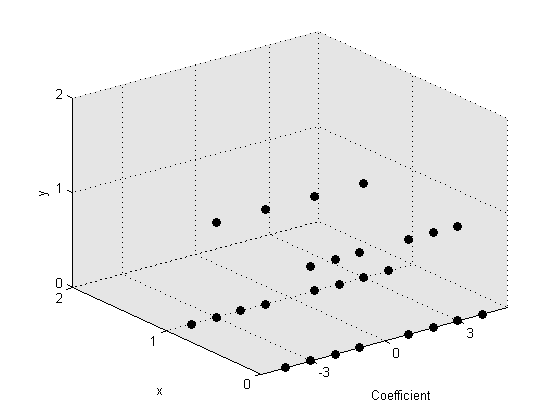
Figure 1. $0^{th}$ border closure

The first border is $\langle x^{2},2xy,y^{2},x^{2}y,xy^{2},4y\rangle$. The first border closure is given by $\langle ax^{2},bxy,cy^{2},dx^{2}y,exy^{2},fy:a,c,d,e\in\mathbb{Z},b\in\langle 2\rangle,f\in\langle 4\rangle$. Figure 2 is an illustration of the same.

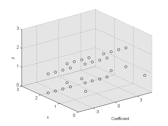
Figure 2. First border closure

For $k\geq 2$ the $k^{th}$ borders are exactly as that of fields. Figure 3 shows the borders for $k=2,3$. Note that the figure depicts the borders and not the border closures.

Figure 3. $2^{nd},3^{rd}$ border closure

We give below certain properties of order ideals, their borders and border closures. These properties are analogous to the case of polynomial rings over fields.

Proposition 3.20.

Let $\mathcal{O}$ be an order ideal and $\partial\mathcal{O}_{m}$ be its monomial border. Then

1. For $k\geq 1$, the $k^{th}$ monomial border closure of $\mathcal{O}$, $\operatorname{Mon}(\overline{\partial^{k}\mathcal{O}})$ is the following disjoint union, $\operatorname{Mon}(\mathcal{O})\cup\partial\mathcal{O}_{m}\cup(\cup_{i=2}^{k}\partial^{k}\mathcal{O})$.

2. For $k\geq 1$, $\partial^{k}\mathcal{O}_{m}$ = $\mathbb{M}_{k}^{n}\cdot\operatorname{Mon}(\mathcal{O})\setminus\mathbb{M}_{<k}^{n}.\operatorname{Mon}(\mathcal{O})$, where $\partial^{k}\mathcal{O}_{m}=\partial^{k}\mathcal{O}$ for $k\geq 2$.

3. A monomial, $x^{\alpha}\in\mathbb{M}^{n}$ is divisible by $x^{\beta}\in\partial\mathcal{O}_{m}$ if and only if $x^{\alpha}\in\mathbb{M}^{n}\setminus\operatorname{Mon}(\mathcal{O})$.

Proof.

(1) The proof is by induction on $k$. For $k=1$, clearly the monomials in the first border closure are elements of the set $\mathcal{O}_{m}\cup\partial\mathcal{O}_{m}$. From the definition of monomial border of $\mathcal{O}$ we have that $\mathcal{O}_{m}$ and $\partial\mathcal{O}_{m}$ are disjoint. Suppose that the claim is true for the $k^{th}$ monomial border closure. For $k+1$, $\overline{\partial^{k+1}\mathcal{O}_{m}}=\overline{\partial^{k}\mathcal{O}_{m}}\cup\partial^{k+1}\mathcal{O}$. It is easy to verify that the sets $\overline{\partial^{k}\mathcal{O}_{m}}$ and $\partial^{k+1}\mathcal{O}$ are disjoint.
(2) The claim follows from the observation that $\partial^{k}\mathcal{O}$ = $\overline{\partial^{k}\mathcal{O}_{m}}\setminus\overline{\partial^{k-1}\mathcal{O}_{m}}$.
(3) We have $x^{\beta}\in\partial\mathcal{O}_{m}$. This implies that there exists $x^{\gamma}\in\mathcal{O}_{m}$ and an indeterminate $x_{i_{0}}$ such that $x^{\beta}=x_{i_{0}}x^{\gamma}$. We have $x_{i_{0}}x^{\gamma}|x^{\alpha}$. If $x^{\alpha}\in\mathcal{O}_{m}$ then $x_{i_{0}}x^{\gamma}\in\mathcal{O}_{m}$ which is a contradiction. Now consider a monomial $x^{\alpha}\in\mathbb{T}^{n}\setminus\mathcal{O}$. Then, $x^{\alpha}\in\partial\mathcal{O}_{m}$ or $x^{\alpha}\in\partial^{k}\mathcal{O}$ for some $k\geq 2$. If $x^{\alpha}\in\partial^{k}\mathcal{O}$ then it implies that there exists a monomial $x^{\gamma}$ of degree $k-1$ and a $x^{\beta}\in\partial\mathcal{O}_{m}$ such that $x^{\alpha}=x^{\gamma}x^{\beta}$. The claim follows. ∎

Now we introduce some concepts that are essential for the division algorithm.

Definition 3.21.

The index of a term $cx^{\alpha}$ w.r.t. an order ideal, $\mathcal{O}$ is defined as

$$\operatorname{ind_{\mathcal{O}}}(cx^{\alpha})=\min\{k\in\mathbb{N}\ |\ cx^{\alpha}\in\overline{\partial^{k}\mathcal{O}}\}.$$

Definition 3.22.

Let $f\in A[x_{1},\ldots,x_{n}]$ be any nonzero polynomial with support, $\operatorname{supp}(f)$, then the index of $f$ w.r.t. an order ideal, $\mathcal{O}$ is defined as

$$\operatorname{ind_{\mathcal{O}}}(f)=\underset{\alpha\in\operatorname{supp}(f)}{\operatorname{max}}\operatorname{ind_{\mathcal{O}}}(c_{\alpha}x^{\alpha}).$$

Example 3.23.

Consider Example 3.5. The set of monic border terms that form the monomial border is $\partial\mathcal{O}_{m}=\{xy,y^{2},$ $x^{3},x^{2}y\}$ and the scalar border is $\partial\mathcal{O}_{s}=\{4x,3y,2x^{2}\}$. Then $\operatorname{ind}_{\mathcal{O}}(3x)=0$, $\operatorname{ind}_{\mathcal{O}}(xy)=1$ and $\operatorname{ind}_{\mathcal{O}}(xy^{2}+8x+7y)=2$.

Example 3.24.

Consider Example 3.6. The monomials that form the monomial border is $\partial\mathcal{O^{\prime}}_{m}=\{x^{3},x^{2}y,x^{2}z,xy^{2},$ $xyz,xz^{2},y^{2},yz,z^{2}\}$ and the scalar border is the set $\partial\mathcal{O^{\prime}}_{s}=\{u_{1}^{2}y,(u_{2}^{2}-3u_{1})z,u_{1}^{2}xy,(u_{2}^{2}-1)xy,u_{1}xz,u_{2}xz\}$. Then
$\operatorname{ind}_{\mathcal{O^{\prime}}}((3u_{2}+u_{2})x)=0$, $\operatorname{ind}_{\mathcal{O^{\prime}}}(u_{1}x^{2}y)=\operatorname{ind}_{\mathcal{O^{\prime}}}((u_{1}^{2}+u_{2})xz)=1$ and $\operatorname{ind}_{\mathcal{O^{\prime}}}(xy^{3}+8x)=2$.

For any polynomial, the terms of highest index are grouped together to form a border form analogous to the leading term in Gröbner bases theory. We define this below.

Definition 3.25.

Let $f\in A[x_{1},\ldots,x_{n}]$ be a nonzero polynomial such that the $\operatorname{ind_{\mathcal{O}}}(f)$ = $i_{0}$. The border form of $f$ w.r.t. $\mathcal{O}$ is defined as

$$\operatorname{BF}_{\mathcal{O}}(f)=\underset{\operatorname{ind_{\mathcal{O}}}(c_{\alpha}x^{\alpha})=i_{0}}{\underset{\alpha\in\operatorname{supp}(f),c_{\alpha}\in A}{\sum}}c_{\alpha}x^{\alpha}\enspace,$$

a polynomial in $A[x_{1},\ldots,x_{n}]$.

Note that unlike leading term of a polynomial in Gröbner bases theory that is always a monomial, border form can be a polynomial. The concept of leading term ideal has an analogous form in border bases theory called the border form ideal.

Definition 3.26.

The border form ideal of an ideal $\mathfrak{a}$ in $A[x_{1},\ldots,x_{n}]$ w.r.t. an order ideal $\mathcal{O}$ is defined as

$$\operatorname{BF}_{\mathcal{O}}(\mathfrak{a})=\langle\operatorname{BF}_{\mathcal{O}}(f)\ |\ f\in\mathfrak{a}\rangle.$$

Example 3.27.

Consider Example  3.5. Let $f=xy^{2}+2x^{2}y^{2}+xy+3x+2$. Then the index of $f$ w.r.t. the order ideal $\mathcal{O}$ is equal to 2. The border form of $f$ is the polynomial, $\operatorname{BF}_{\mathcal{O}}(f)=xy^{2}+2x^{2}y^{2}$.

Example 3.28.

Consider Example  3.6. Let $f=2xy^{2}+(u_{1}-u_{2})xz+3x+2$. Then the index of $f$ w.r.t. the order ideal $\mathcal{O^{\prime}}$ is equal to 2. The border form of $f$ is the polynomial, $\operatorname{BF}_{\mathcal{O^{\prime}}}(f)=2xy^{2}+(u_{1}-u_{2})xz$.

We now give the definition of border prebasis for an order ideal, $\mathcal{O}$.

Definition 3.29.

Let $\mathcal{O}$ be an order ideal, and $\partial\mathcal{O}=\{c_{1}x^{\alpha_{1}},\ldots,c_{s}x^{\alpha_{s}}\}$ be its border. Let $C_{x^{\alpha_{i}}}$ be the set of coset representatives of $A/\mathcal{I}_{x^{\alpha_{i}}}$. A finite set of polynomials $G$ = $\{g_{1},\ldots,g_{s}\}\subseteq A[x_{1},\ldots,x_{n}]$ is said to be an $\mathcal{O}$-border prebasis if $g_{i}=c_{i}x^{\alpha_{i}}-h_{i}$, where $h_{i}\in A[x_{1},\ldots,x_{n}]$ satisfying $\mathrm{Ter}(h_{i})\subseteq\mathcal{O}\setminus\{ax^{\alpha_{i}}\ |\ a\in C_{x^{\alpha_{i}}}\}$, $i=1,\ldots,s$.

Example 3.30.

We consider Example 3.5. The set $G=\{g_{1},\ldots,g_{7}\}$, where $g_{1}=xy-x$, $g_{2}=y^{2}-y$, $g_{3}=x^{3}-2y$, $g_{4}=x^{2}y-x^{2}+10$, $g_{5}=4x-2y$, $g_{6}=3y-3x$ and $g_{7}=2x^{2}-x+5$ is an $\mathcal{O}$-border prebasis but it is not acyclic. Let $G^{\prime}=\{g^{\prime}_{1},\ldots,g^{\prime}_{7}\}$ where $g^{\prime}_{1}=xy-x$, $g^{\prime}_{2}=y^{2}-y$, $g^{\prime}_{3}=x^{3}-x^{2}+6$, $g^{\prime}_{4}=x^{2}y-y+5$, $g^{\prime}_{5}=4x-7$, $g^{\prime}_{6}=3y-x$ and $g^{\prime}_{7}=2x^{2}-2y-3x$ which is also a $\mathcal{O}$-border prebasis but it is acyclic since the permutation of $G^{\prime}$, $\{g^{\prime}_{1},g^{\prime}_{2},g^{\prime}_{3},g^{\prime}_{4},g^{\prime}_{7},g^{\prime}_{6},g^{\prime}_{5}\}$ satisfies the acyclicity condition.

Example 3.31.

Consider Example 3.6. The set $G=\\ \{g_{1},\ldots,g_{15}\}$, where $g_{1}=x^{3}-3$, $g_{2}=x^{2}y-3u_{1}y$, $g_{3}=x^{2}z-2z$, $g_{4}=xy^{2}-x+10$, $g_{5}=xyz-11xy$, $g_{6}=xz^{2}-u_{2}u_{1}^{2}x^{2}$, $g_{7}=y^{2}-x+u_{1}u_{2}$, $g_{8}=yz-3y+2$, $g_{9}=z^{2}+5xz+11u_{1}x$, $g_{10}=u_{1}^{2}y+u_{2}x+3$, $g_{11}=(u_{2}^{2}-3u_{1})z-u_{2}^{2}y$, $g_{12}=u_{1}^{2}xy+3u_{1}x-2z$, $g_{13}=(u_{2}^{2}-1)xy+2x^{2}$, $g_{14}=u_{1}xz+3u_{1}x^{2}$, $g_{15}=u_{2}xz+2u_{1}xy+4x^{2}-4z-10u_{1}y+14$ is an acyclic $\mathcal{O}$-border prebasis since the following permutation of $G$, $\{g_{1},g_{2},g_{3},g_{4},g_{5},g_{6},g_{7},g_{8},g_{9},g_{14},g_{15},g_{13},g_{12},g_{11},g_{10}\}$ satisfies the acyclicity condition.

Note that unlike in fields, for a monomial in the border of $\mathcal{O}$, we can have more than one polynomial in the $\mathcal{O}$-border prebasis but only one polynomial corresponding to a term in the border. With the definition of $\mathcal{O}$-border prebasis, we now give a procedure for division of any polynomial in $A[x_{1},\ldots,x_{n}]$ with the $\mathcal{O}$-border prebasis.

Algorithm 3.32.

Let $\mathcal{O}$ be an order ideal. Let $\operatorname{Mon}(\mathcal{O})=\{x^{\alpha_{1}},\ldots,x^{\alpha_{t}}\}$ be its monomial part. Let $\partial\mathcal{O}_{m}=\{x^{\beta_{1}},\ldots,x^{\beta_{s^{\prime}}}\}$ and $\partial\mathcal{O}_{s}=\{c_{s^{\prime}+1}x^{\beta_{s^{\prime}+1}},\ldots,c_{s}x^{\beta_{s}}\}$ be its monomial border and scalar border respectively. Let $G=\{g_{1},\ldots,g_{s}\}\subseteq A[x_{1},\ldots,x_{n}]$ be an $\mathcal{O}$-border prebasis. For $f\in A[x_{1},\ldots,x_{n}]$ we perform the following steps.

1. Initialize $f_{1}=\ldots=f_{s}=0$, $a_{1}=\ldots=a_{t}=0$ and $h=f$.

2. If $h=0$ return ($f_{1},\ldots,f_{s},a_{1},\ldots,a_{t}$).

3. If $\operatorname{ind}_{\mathcal{O}}(h)$ = $0$ then find $b_{1},\ldots,b_{t}\in A$ such that $h=b_{1}x^{\alpha_{1}}+\ldots+b_{t}x^{\alpha_{t}}$. Set $a_{i}=b_{i}$ for each $1\leq i\leq t$. Return ($f_{1},\dots,f_{s},a_{1},\ldots,a_{t}$).

4. If $\operatorname{ind}_{\mathcal{O}}(h)$ = $1$ and $h$ contains a term $dx^{\beta}$ such that $x^{\beta}\in\partial\mathcal{O}_{m}$ then goto Step 5. Else, let $h$ = $d_{1}x^{\gamma_{1}}+\ldots+d_{j}x^{\gamma_{j}}$ such that $\operatorname{ind}_{\mathcal{O}}(h)=\operatorname{ind}_{\mathcal{O}}(d_{1}x^{\gamma_{1}})$ and $\operatorname{ind}_{\mathcal{O}}(d_{1}x^{\gamma_{1}})\geq\ldots\geq\operatorname{ind}_{\mathcal{O}}(d_{j}x^{\gamma_{j}})$. Find $b_{\mu+1},\ldots,b_{s}\in A$ such that $d_{1}x^{\gamma_{1}}=b_{s^{\prime}+1}(c_{s^{\prime}+1}x^{\beta_{s^{\prime}+1}})+\ldots+b_{s}(c_{s}x^{\beta_{s}})$. Subtract $b_{s^{\prime}+1}g_{s^{\prime}+1}+\ldots+b_{s}g_{s}$ from $h$, add $b_{i}\ to\ f_{i}$ for $s^{\prime}+1\leq i\leq s$ and return to Step 2.

5. Else, let $h$ = $d_{1}x^{\gamma_{1}}+\ldots+d_{j}x^{\gamma_{j}}$ such that $\operatorname{ind}_{\mathcal{O}}(h)=\operatorname{ind}_{\mathcal{O}}(x^{\gamma_{1}})$ and $\operatorname{ind}_{\mathcal{O}}(d_{1}x^{\gamma_{1}})\geq\ldots\geq\operatorname{ind}_{\mathcal{O}}(d_{j}x^{\gamma_{j}})$. Determine $x^{\beta_{i}}\in\partial\mathcal{O}_{m}$ with the smallest $i$ such that $x^{\gamma_{i}}=x^{\mu}x^{\beta_{i}}$ and $\operatorname{deg}(x^{\mu})=\operatorname{ind}_{\mathcal{O}}(h)-1$. Subtract $d_{1}x^{\mu}g_{i}$ from $h$, add $d_{1}x^{\mu}$ to $f_{i}$ and return to Step 2.

This procedure over rings differs from the case of fields only in Step 4. The termination of the above method is not assured because of the possibility that for a given polynomial, $f$, a monomial in its support identified with index $0$ in Step 3 may again have an index 1 after Step 4. Therefore, we cannot assume the reduction in index values at every step of the procedure.

4. Acyclic Border Prebases and Termination of Border Division Algorithm

Here, we identify a special class of $\mathcal{O}$-border prebases called acyclic $\mathcal{O}$-border prebases for which the termination of the border division algorithm can be established.

Definition 4.1.

A $\mathcal{O}$-border prebasis $G$ = $\{g_{1},\ldots,g_{s}\}$ is said to be acyclic if there exists a permutation of $G$, $\{g_{i_{1}},\ldots,g_{i_{s}}\}$ such that for any $g_{i_{j}}$, $g_{i_{k}}$, where $j\lneq k$, exactly one of the following conditions are satisfied

1. $c_{j}\operatorname{BF}_{\mathcal{O}}(g_{i_{j}})=c_{k}\operatorname{BF}_{\mathcal{O}}(g_{i_{k}})$ for any $c_{j},c_{k}\in A$ or

2. $d_{j}x^{\alpha_{j}}\in\partial\mathcal{O}$ and $d_{j}x^{\alpha_{j}}\in\operatorname{supp}(g_{i_{j}})$ implies $c_{k}x^{\alpha_{j}}\notin\operatorname{supp}(g_{i_{k}})$ for some $c_{k},d_{j}\in A$.

The ordered set of acyclic $\mathcal{O}$-border prebasis that satisfies the permutation given above is called a ‘well ordered’ acyclic $\mathcal{O}$-border prebasis. We now show the correctness and termination of Algorithm 3.32 when the $\mathcal{O}$-border prebasis is acyclic.

Proposition 4.2.

(Border Division Algorithm) Consider a polynomial $f\in A[x_{1},\ldots,x_{n}]$. If the $\mathcal{O}$-border prebasis $G=\{g_{1},\ldots,g_{s}\}$ is acyclic, then Algorithm  3.32 terminates for $f$ and returns a tuple,

$$(f_{1},\ldots,f_{s},a_{1},\ldots,a_{t})\in(A[x_{1},\ldots,x_{n}])^{s}\times A^{t}$$

such that

$$f=f_{1}g_{1}+\ldots+f_{s}g_{s}+a_{1}x^{\alpha_{1}}+\ldots+a_{t}x^{\alpha_{t}},$$

and $\operatorname{deg}(f_{i})\leq\operatorname{ind}_{\mathcal{O}}(f)$, for $i=1,\ldots,s$ with $f_{i}g_{i}\neq 0$.

Proof.

We first describe the execution of the algorithm. In Step 4, $\operatorname{ind}_{\mathcal{O}}(d_{1}x^{\gamma_{1}})=1$ and $d_{1}x^{\gamma_{1}}\in\operatorname{Span}_{A}(\langle\partial\mathcal{O}\rangle_{A})$. This implies that $d_{1}\in\mathcal{I}_{x^{\gamma_{1}}}$, where $\mathcal{I}_{x^{\gamma_{1}}}$ is an ideal generated by $\langle u_{1},\ldots,u_{k}\rangle$, $\ u_{i}x^{\gamma_{1}}\in\partial\mathcal{O}_{s}$, $1\leq i\leq k$. Thus, there exists $l_{1},\ldots,l_{k}\in A$ such that $d_{1}=\sum_{i=1}^{k}l_{i}u_{i}$. Hence, $d_{1}x^{\gamma_{1}}=\sum_{s^{\prime}+1}^{s}b_{i}(c_{i}x^{\beta_{i}})$, where $c_{i}x^{\beta_{i}}\in\partial\mathcal{O}_{s}$ and $b_{i}=l_{j}$ when $c_{i}x^{\beta_{i}}=u_{j}x^{\gamma_{1}}$ for some $j\in\{1,\ldots,k\}$, and $b_{i}=0$, otherwise. The other steps, due to the absence of scalar border terms, mimics the border basis division in fields (Kehrein & Kreuzer, 2005, Proposition 3). We prove that the representation,

$$f=f_{1}g_{1}+\ldots+f_{s}g_{s}+a_{1}x^{\alpha_{1}}+\ldots+a_{t}x^{\alpha_{t}}+h,$$

computed by the algorithm is valid in every step. Clearly, it is satisfied in Step 1. In Step 4 we subtract $(b_{s^{\prime}+1}g_{s^{\prime}+1}+\ldots+b_{s}g_{s})$ from $h$. These $b_{i}$s are then added to $f_{i}$s, i.e. $f_{i}=f_{i}+b_{i}$, $s^{\prime}+1\leq i\leq s$. Similarly in Step 5, from $h$ we subtract $d_{1}x^{\mu}g_{i}$ and we add $d_{1}x^{\mu}$ to $f_{i}$. The constants $a_{1},\ldots,a_{t}$ are modified only in Step 3. The representation of $f$ is valid because $\operatorname{ind_{\mathcal{O}}}(h)=0$. If the algorithm terminates, $h=0$ and we have a valid representation.

Now we prove that $\operatorname{deg}(f_{i})\leq\operatorname{ind}_{\mathcal{O}}(f)$ for all $i=1,\ldots,s$. In Step 5 of the algorithm, where we divide using the monomial border, our choice of the term $d_{1}x^{\mu}$ is such that
$\operatorname{deg}(dx^{\mu})=\operatorname{ind}_{\mathcal{O}}(h)-1$. In Step 4, where we divide using the scalar border, the index of the intermediate polynomial, $h$ is 1. The $b_{i}$, $i=1,\ldots,s$ are constants and the degree of $f_{i}$, $i=1,\ldots,s$ are therefore zero. All the other steps in the algorithm do not affect $f_{i}$, $i=1,\ldots,s$. Also, in the algorithm the index of the intermediate polynomial, $h$ never increases. From the above steps, the inequality $\operatorname{deg}(f_{i})\leq\operatorname{ind}_{\mathcal{O}}(f)-1$ for all $i=1,\ldots,s$ follows.

Next, we prove that the algorithm terminates on all inputs. In Step 4, $\operatorname{ind_{\mathcal{O}}}(h)=1$ and $\mathrm{Ter}(h)\subseteq$ $\operatorname{Span}_{A}(\operatorname{Mon}(\mathcal{O}))\cup\operatorname{Span}_{A}(\partial\mathcal{O}_{s})$ = $\operatorname{Span}_{A}(\operatorname{Mon}(\mathcal{O}))$. We claim that Step 4 terminates after a finite number of steps for an acyclic $\mathcal{O}$-border prebasis. Let $h=d_{1}x^{\alpha_{1}}+\ldots+d_{t}x^{\alpha_{t}}$. For simplicity, let us assume that the acyclic $\mathcal{O}$-border prebasis, $G$ is well ordered. It can easily be seen that $g_{1}$ will be used atmost once in Step 4, while $g_{2}$ will be used at most twice ($h\xrightarrow{g_{2}}h_{1}\xrightarrow{G\setminus\{g_{1},g_{2}\}}_{+}h_{2}\xrightarrow{g_{1}}h_{3}\xrightarrow{G\setminus\{g_{1},g_{2}\}}_{+}h_{4}\xrightarrow{g_{2}}h_{5}$). Similarly, any $g_{i}$ will be used atmost $\operatorname{O}\bigl{(}i^{2})$ times. For the set $G$, therefore Step 4 is executed at most $\operatorname{O}\bigl{(}s^{3})$ times. All the other steps of the division correspond to either order ideal, monomial border or the $k^{th}$ order border, $k\gneq 1$ and therefore mimic the border division in fields. Hence, the termination is guaranteed by (Kehrein & Kreuzer, 2005, Proposition 3). ∎

The border division algorithm gives us the remainder upon division by an acyclic $\mathcal{O}$-border prebasis as a part of its output. We now give a formal definition for remainder.

Definition 4.3.

Let $\mathcal{O}$ be an order ideal and $\operatorname{Mon}(\mathcal{O})=\{x^{\alpha_{1}},\ldots,x^{\alpha_{t}}\}$, its monomial part. Let $G=\{g_{1},\ldots,g_{s}\}$ be the $\mathcal{O}$-border prebasis. The $\mathcal{O}$-remainder of a polynomial $f$ w.r.t. $G$, if it exists, is given as

$$\operatorname{rem}_{\mathcal{O},G}(f)=a_{1}x^{\alpha_{1}}+\ldots+a_{t}x^{\alpha_{t}},$$

where $f=f_{1}g_{1}+\ldots+f_{s}g_{s}+a_{1}x^{\alpha_{1}}+\ldots+a_{t}x^{\alpha_{t}}$ and $a_{i}\in A$ for all $i=1,\ldots,t$ is a representation computed by the border division algorithm whenever the algorithm terminates.

5. Order Span and Acyclic Border Bases

Consider the case when $A[x_{1},\ldots,x_{n}]/\mathfrak{a}$ is finitely generated. Using the order function we define a generating set for $A[x_{1},\ldots,x_{n}]/\mathfrak{a}$ that also satisfies a weaker form of the linear independence property.

Definition 5.1 (Order span).

Let $\mathfrak{a}$ be an ideal and let $\mathcal{I}$ be a proper order function and $\mathcal{B}=\{x^{\alpha_{1}},\ldots,x^{\alpha_{m}}\}$ be a finite set of monomials of size $m$ such that $x^{\alpha}\notin\mathcal{B}$ if and only if $\mathcal{I}_{x^{\alpha}}=\langle 1\rangle$, where $x^{\alpha}\in\mathbb{M}^{n}$. Let $C_{\mathcal{I}_{x^{\alpha}}}$ be the coset representatives of the equivalence classes of $A/\mathcal{I}_{x^{\alpha}}$. Then we say the set of residue classes of $\mathcal{B}$ forms an order span for $A[x_{1},\ldots,x_{n}]/\mathfrak{a}$ w.r.t. $\mathcal{I}$ if it satisfies the following properties.

1. $\mathcal{B}+\mathfrak{a}$ generates $A[x_{1},\ldots,x_{n}]/\mathfrak{a}$ as an $A$-module and

   $$A[x_{1},\ldots,x_{n}]/\mathfrak{a}=\{\sum\limits_{i=1}^{m}a_{i}x^{\alpha_{i}}+\mathfrak{a}\ |\ a_{i}\in C_{\mathcal{I}_{x^{\alpha_{i}}}},x^{\alpha_{i}}\in\mathcal{B}\}.$$

2. If $\sum_{i=1}^{m}a_{i}x^{\alpha_{i}}+\mathfrak{a}=0$, where $m\in\mathbb{N}$, $x^{\alpha_{i}}\in\mathcal{B}$ and $a_{i}\neq 0$ for all $i=1,\ldots,m$, then for some $j\in\{1,\ldots,m\}$, $a_{j}\in\mathcal{I}_{x^{\alpha_{j}}}$.

3. If there exists an order function $\mathcal{I}^{{}^{\prime}}$ such that $\mathcal{I}^{{}^{\prime}}_{x^{\alpha}}\subseteq\mathcal{I}_{x^{\alpha}}$ for some $x^{\alpha}\in\mathbb{M}^{n}$ and $\mathcal{B}^{{}^{\prime}}=\{x^{\alpha}:\mathcal{I}^{{}^{\prime}}_{x^{\alpha}}\neq\langle 1\rangle\}$ satisfies (i) and (ii) w.r.t. $\mathcal{I}^{{}^{\prime}}$, then $\mathcal{I}^{{}^{\prime}}=\mathcal{I}$.

Remark 5.2.

The linear independence property requires that if $\sum_{i=1}^{k}a_{i}x^{\alpha_{i}}+\mathfrak{a}=0$ then for all $i\in\{1,\ldots,k\}$, $a_{i}\in\mathcal{I}_{x^{\alpha_{i}}}$. Therefore, the second condition in Definition 5.1 is a weaker form of the linear independence property. In fact, in the case of fields and residue class rings with a free $A$-module representation, the second condition automatically implies the linear independence property.

Remark 5.3.

The third condition in Definition 5.1 can be interpreted as a minimality condition on the spanning set. Over fields, linear independence of the spanning set ensures minimality but over rings it has to be specified separately. Consider the ideal $\mathfrak{a}=\langle 4x_{1},{x_{1}}^{2},x_{2}\rangle$ in $\mathbb{Z}[x_{1},x_{2}]$. Let $\mathcal{I}$ and $\mathcal{I}^{{}^{\prime}}$ be two order functions. Define $\mathcal{I}_{1}={0},\mathcal{I}_{x_{1}}=\langle 2\rangle$ and for all the other monomials $x^{\alpha}$, $\mathcal{I}_{x^{\alpha}}=\langle 1\rangle$. Similarly define $\mathcal{I}^{{}^{\prime}}_{1}={0},\mathcal{I}^{{}^{\prime}}_{x_{1}}=\langle 4\rangle$ and for all the other $x^{\alpha}\in\mathbb{M}^{2}$, $\mathcal{I}^{{}^{\prime}}_{x^{\alpha}}=\langle 1\rangle$. Both $\mathcal{I}$ and $\mathcal{I}^{{}^{\prime}}$ satisfy the first two conditions of the order span. However, since $\mathcal{I}^{{}^{\prime}}_{x_{1}}(=\langle 4\rangle)\subsetneq\mathcal{I}_{x_{1}}(=\langle 2\rangle)$, it is w.r.t. the second order function, $\mathcal{I}^{{}^{\prime}}$ that we define the order span of $\mathbb{Z}[x_{1},x_{2}]/\langle 4x_{1},{x_{1}}^{2},x_{2}\rangle$.

Corollary 5.4.

Let $\mathfrak{a}$ be an ideal such that $A[x_{1},\ldots,x_{n}]/\mathfrak{a}$ is finitely generated. Let $G=\{g_{1},\ldots,g_{t}\}$ be a Gröbner basis of an ideal $\mathfrak{a}$ and $\mathcal{I}^{(G)}$ the order function fixed by $G$. Then,

1. The order function $\mathcal{I}^{(G)}$ is proper,

2. The finite order span of $A[x_{1},\ldots,x_{n}]/\mathfrak{a}$ w.r.t. $\mathcal{I}^{(G)}$ is given by

   $$\mathcal{B}=\{x^{\alpha}:\mathrm{lt}(g_{i})\nmid ax^{\alpha},\text{ for some nonzero }a\in A,g_{i}\in G\}$$

We now provide a better interpretation of the mapping described by (1) in terms of order span.

Proposition 5.5.

Let $\mathfrak{a}$ be an ideal in $A[x_{1},\ldots,x_{n}]$. Let $\mathcal{I}$ be a proper order function and $\mathcal{B}=\{x^{\alpha_{1}},\ldots,x^{\alpha_{m}}\}$ be a finite set of monomials of size $m$ such that if $x^{\alpha}\notin\mathcal{B}$, $\mathcal{I}_{x^{\alpha}}=\langle 1\rangle$, where $x^{\alpha}\in\mathbb{M}^{n}$. Consider a mapping,

$$\begin{split}\phi:A[x_{1},\ldots,x_{n}]/\mathfrak{a}&\longrightarrow A/\mathcal{I}_{{x^{\alpha_{1}}}}\times\cdots\times A/\mathcal{I}_{{x^{\alpha_{m}}}}\\ f+\mathfrak{a}&\longmapsto(c_{1}+\mathcal{I}_{{x^{\alpha_{1}}}},\cdots,c_{m}+\mathcal{I}_{x^{\alpha_{m}}}),\end{split}$$

where $c_{i}\in C_{\mathcal{I}_{x^{\alpha_{i}}}}$ for all $i\in\{1,\ldots,m\}$. Then, $\phi$ is an isomorphism if $\mathcal{B}$ forms an order span for $A[x_{1},\ldots,x_{n}]/\mathfrak{a}$.

Proof.

Let $\mathcal{B}$ form an order span for $A[x_{1},\ldots,x_{n}]/\mathfrak{a}$. We first show that the mapping $\phi$ is well defined. Consider a polynomial $f\in A[x_{1},\ldots,x_{n}]$. Suppose

$$\phi(f+\mathfrak{a}) =(c_{1}+\mathcal{I}_{{x^{\alpha_{1}}}},\cdots,c_{m}+\mathcal{I}_{x^{\alpha_{m}}})\text{ and }$$

$$\phi(f+\mathfrak{a}) =(c^{\prime}_{1}+\mathcal{I}_{{x^{\alpha_{1}}}},\cdots,c^{\prime}_{m}+\mathcal{I}_{x^{\alpha_{m}}}),$$

where $c_{i}$, $c^{\prime}_{i}$ $\in C_{\mathcal{I}_{x^{\alpha_{i}}}}$, for all $i=1,\ldots,m$. This implies $(c_{i}-c^{\prime}_{i})\in\mathcal{I}_{{x^{\alpha_{i}}}}$, $i=1,\ldots,m$. Since the difference of two different coset representatives cannot give the zero coset, we have $c_{i}=c^{\prime}_{i}$ for all $i=1,\ldots,m$. Thus $\phi$ is well defined.

Clearly, $\phi$ is a surjective map by construction. We now have to prove that $\phi$ is an injective mapping. Consider a polynomial $f\in A[x_{1},\ldots,x_{n}]$ such that $\phi(f+\mathfrak{a})=(0,\ldots,0)$. Let us assume that $f\notin\mathfrak{a}$. Since $\mathcal{B}$ forms an order span for $A[x_{1},\ldots,x_{n}]/\mathfrak{a}$, we can obtain $c_{i}\in C_{\mathcal{I}_{x^{\alpha_{i}}}}$, $i=1,\ldots,m$ such that $f=\sum\limits_{i=1}^{m}c_{i}x^{\alpha_{i}}$ mod $\mathfrak{a}$. Further, atleast one of the $c_{i}$, $i\in\{1,\ldots,m\}$, is nonzero. This implies that $\phi(f+\mathfrak{a})$ also maps to $(c_{1},\ldots,c_{m})$. Therefore $\phi$ is not a well defined mapping. This is a contradiction and $f\in\mathfrak{a}$. Thus, the kernel of $\phi$, $\ker(\phi)=\{0+\mathfrak{a}\}$. This implies that $\phi$ is an injective mapping. Hence, it follows that $\phi$ is an isomorphism. ∎

Definition 5.6.

Let $\mathfrak{a}$ be an ideal such that $A[x_{1},\ldots,x_{n}]/\mathfrak{a}$ is a finitely generated $A$-module. Let $\mathcal{O}$ be an order ideal and $G=\{g_{1},\ldots,g_{s}\}$ be an acyclic $\mathcal{O}$-border prebasis consisting of polynomials in $\mathfrak{a}$. $G$ is an acyclic $\mathcal{O}$-border basis of $\mathfrak{a}$ if $\operatorname{Mon}(\mathcal{O})$ is an order span of $A[x_{1},\ldots,x_{n}]/\mathfrak{a}$.

The next proposition shows that these polynomials indeed generate the ideal in $\mathfrak{a}$.

Proposition 5.7.

Let $\mathfrak{a}$ be an ideal such that $A[x_{1},\ldots,x_{n}]/\mathfrak{a}$ is finitely generated as an $A$-module. Let $\mathcal{O}$ be an order ideal and let $G=\{g_{1},\ldots,g_{s}\}$ be an acyclic $\mathcal{O}$-border basis for $\mathfrak{a}$. Then $\mathfrak{a}$ is generated by $G$.

Proof.

Let $\operatorname{Mon}(\mathcal{O})=\{x^{\alpha_{1}},\ldots,x^{\alpha_{t}}\}$ be the monomial part of $\mathcal{O}$ and $G=\{g_{1},\ldots,g_{s}\}$ be an acyclic $\mathcal{O}$-border basis of $\mathfrak{a}$. Consider, $f\in\mathfrak{a}$. By Algorithm 4.2, we have $f_{1},\ldots,f_{s}\in A[x_{1},\ldots,x_{n}]$ and $a_{1},\ldots,a_{t}\in A$ such that

$$f=f_{1}g_{1}+\ldots+f_{s}g_{s}+a_{1}x^{\alpha_{1}}+\ldots+a_{t}x^{\alpha_{t}}.$$ (2)

Now, $f-\sum_{i=1}^{s}f_{i}g_{i}\in\mathfrak{a}$. This implies, $\sum_{i=1}^{t}a_{i}x^{\alpha_{i}}\in\mathfrak{a}$. Let $h=\sum_{i=1}^{t}a_{i}x^{\alpha_{i}}$. Suppose $h\neq 0$, then $a_{i}\notin\mathcal{I}_{x^{\alpha_{i}}}\setminus\{0\}$, for all $i=1,\ldots,t$. If $a_{i}\in\mathcal{I}_{x^{\alpha_{i}}}$, for all $i=1,\ldots,t$, then $\operatorname{ind_{\mathcal{O}}}(h)=1$. Then, (2) is not a valid output of Algorithm  4.2. But we are also given that $G$ is an acyclic border basis of $\mathfrak{a}$. The order span property of border basis implies that if $\sum_{i=1}^{t}a_{i}x^{\alpha_{i}}\in\mathfrak{a}$ for $a_{i}\neq 0$ for all $i=1,\ldots,t$, then $a_{i}\in\mathcal{I}_{x^{\alpha_{i}}}$ for some $i\in\{1,\ldots,t\}$. This is a contradiction. Hence, $h=0$. We have, $f=\sum_{i=1}^{s}f_{i}g_{i}$. The other inclusion follows from the fact that $G\subseteq\mathfrak{a}$. ∎

We need to verify if an acyclic $\mathcal{O}$-border basis exists for every ideal, $\mathfrak{a}$ in $A[x_{1},\ldots,x_{n}]$. We first address, below, whether an acylic $\mathcal{O}$-border basis for $\mathfrak{a}$ given an order ideal, $\mathcal{O}$, exists. We also prove the uniqueness of the acyclic $\mathcal{O}$-border basis.

Theorem 5.8.

Let $\mathcal{O}$ be an order ideal, and let $\mathfrak{a}$ be an ideal such that $A[x_{1},\ldots,x_{n}]/\mathfrak{a}$ is a finitely generated $A$-module. If $\operatorname{Mon}(\mathcal{O})$ is an order span then there exists a unique acyclic $\mathcal{O}$-border basis for $\mathfrak{a}$.

Proof.

Let $\operatorname{Mon}(\mathcal{O})=\{x^{\alpha_{1}},\ldots,x^{\alpha_{t}}\}$ be the monomial part of $\mathcal{O}$, and let $\partial\mathcal{O}=\{c_{1}x^{\beta_{1}},\ldots,c_{s}x^{\beta_{s}}\}$ be the border of $\mathcal{O}$. We now prove that an $\mathcal{O}$-border basis exists for $\mathfrak{a}$. Since $\operatorname{Mon}(\mathcal{O})$ is an order span basis, for each $c_{i}x^{\beta_{i}}\in\partial\mathcal{O}$ one can find $a_{j}^{(i)}x^{\alpha_{i}}s\in\mathcal{O}$ such that $c_{i}x^{\beta_{i}}=\sum_{j=1}^{t}a^{(i)}_{j}x^{\alpha_{j}}\text{ mod }\mathfrak{a}$. We define $G$ as

$$G=\{c_{i}x^{\beta_{i}}-\sum_{j=1}^{t}a^{(i)}_{j}x^{\alpha_{j}}\ |\ 1\leq i\leq s\}.$$

Clearly, $G$ is an acyclic $\mathcal{O}$-border prebasis. Now, $G\subseteq\mathfrak{a}$ and $A[x_{1},\ldots,x_{n}]/\mathfrak{a}=\{\sum a_{i}x^{\alpha_{i}}+\mathfrak{a}\ |\ x^{\alpha_{i}}\in\operatorname{Mon}(\mathcal{O})\text{ and }a_{i}\in A\}$. Hence, $G$ is an $\mathcal{O}$-border basis of $\mathfrak{a}$.

To prove the uniqueness of $\mathcal{O}$-border basis, consider two acyclic $\mathcal{O}$-border bases for $\mathfrak{a}$. Let $G=\{g_{1},\ldots,g_{t}\}$ and $G=\{g^{\prime}_{1},\ldots,g^{\prime}_{t}\}$ such that

$$\begin{split}&g_{i}=c_{i}x^{\beta_{i}}-\sum_{j=1}^{t}a^{(i)}_{j}x^{\alpha_{j}},\text{ where each }a_{j}^{(i)}x^{\alpha_{j}}\in\mathcal{O}\text{ and},\\ &g^{\prime}_{i}=c_{i}x^{\beta_{i}}-\sum_{j=1}^{t}a^{\prime(i)}_{j}x^{\alpha_{j}},\text{ where each }a^{\prime(i)}_{j}x^{\alpha_{j}}\in\mathcal{O}.\\ \end{split}$$

We have,

$$g_{i}-g^{\prime}_{i}=\sum_{j=1}^{t}a^{(i)}_{j}x^{\alpha_{j}}-\sum_{j=1}^{t}a^{\prime(i)}_{j}x^{\alpha_{j}}\in\mathfrak{a}.\\$$

This implies,

$$\sum_{j=1}^{t}(a^{(i)}_{j}-a^{\prime(i)}_{j})x^{\alpha_{j}}\in\mathfrak{a}.$$

Since $a^{(i)}_{j}$ and $a^{\prime(i)}_{j}$ are coset representatives of $A/\mathcal{I}_{x^{\alpha_{j}}}$ and the difference of two different cosets cannot be a zero coset, we have $a^{(i)}_{j}=a^{\prime(i)}_{j}$. Therefore, $g_{i}=g^{\prime}_{i}$. Hence, the acyclic $\mathcal{O}$-border basis of $\mathfrak{a}$ is unique. ∎

Thus, the question of existence of a border basis for an ideal reduces to the following questions. Given an ideal $\mathfrak{a}$, (i) does there always exist a proper order function, $\mathcal{I}$ such that the monomial part of the order ideal, $\operatorname{Mon}(\mathcal{O})$ constructed from $\mathcal{I}$ forms an order span for $A[x_{1},\ldots,x_{n}]/\mathfrak{a}$ and (ii) will the corresponding $\mathcal{O}$-border basis be acyclic. We use the theory of Gröbner bases to establish the result.

Theorem 5.9.

Given an ideal $\mathfrak{a}$ such that $A[x_{1},\ldots,x_{n}]/\mathfrak{a}$ is finitely generated as an $A$-module, there always exists an acyclic border basis of $\mathfrak{a}$ corresponding to some order ideal, $\mathcal{O}$.

Proof.

Let $\prec$ be a monomial order on $A[x_{1},\ldots,x_{n}]$. Let $G^{\prime}=\{g^{\prime}_{1},\ldots,g^{\prime}_{t}\}$ be a Gröbner basis of $\mathfrak{a}$. Consider the order function fixed by $G$, $\mathcal{I}^{(G)}$. Since $A[x_{1},\ldots,x_{n}]/\mathfrak{a}$ is finitely generated, the mapping is proper. Let $\mathcal{O}_{\prec}$ be the order ideal corresponding to $\mathcal{I}^{(G)}$. It follows from Corollary 5.4 that $\operatorname{Mon}(\mathcal{O}_{\prec})$ forms an order span. Let $\partial\mathcal{O_{\prec}}=\{c_{1}x^{\beta_{1}},\ldots,c_{s}x^{\beta_{s}}\}$ be the border of $\mathcal{O}_{\prec}$. Let $G$ be the $\mathcal{O}_{\prec}$-border prebasis constructed along the same lines as in the proof of Theorem  5.8. Therefore, each polynomial $g_{i}$ in $G$ is of the form,

$$g_{i}=c_{i}x^{\beta_{i}}-\sum_{j=1}^{t}a^{(i)}_{j}x^{\alpha_{j}},\hskip 3.0pti=1,\ldots,s,$$

where $c_{i}x^{\beta_{i}}\in\partial\mathcal{O}$ and each $a^{(i)}_{j}x^{\alpha_{j}}\in\mathcal{O}$.

For any $g_{i}\in G$, monomial ordering imposes that for every nonzero $a^{(i)}_{j}x^{\alpha_{j}}$, $x^{\alpha_{j}}\prec x^{\beta_{i}}$. Also, for two distinct border terms $c_{i}x^{\beta_{i}}$ and $c_{j}x^{\beta_{j}}$ such that $x^{\beta_{i}}\neq x^{\beta_{j}}$, either $x^{\beta_{i}}\prec x^{\beta_{j}}\text{ or }x^{\beta_{j}}\prec x^{\beta_{i}}$. The acyclic property of $G$ follows from these two observations. Theorem 5.8 implies that $G$ forms a unique acyclic $\mathcal{O_{\prec}}$-border basis for $\mathfrak{a}$. ∎

For any polynomial $f\in A[x_{1},\ldots,x_{n}]$, given an acylic $\mathcal{O}$-border prebasis, $G$ and an order ideal, $\mathcal{O}$, $\mathcal{O}$-remainder of $f$ is denoted by $\operatorname{rem_{\mathcal{O},G}}(f)$ (Definition 4.3).

Proposition 5.10.

Let $\mathfrak{a}\subseteq A[x_{1},\ldots,x_{n}]$ be an ideal such that $A[x_{1},\ldots,x_{n}]/\mathfrak{a}$ is finitely generated as an $A$-module and $G\subseteq\mathfrak{a}$ be an acyclic $\mathcal{O}$-border basis of $\mathfrak{a}$. For any $f\in A[x_{1},\ldots,x_{n}]$, $f\in\mathfrak{a}$ if and only if $\mathrm{rem}_{\mathcal{O},G}(f)=0$.

Proof.

Let $\operatorname{Mon}(\mathcal{O})=\{x^{\alpha_{1}},\ldots,x^{\alpha_{t}}\}$ be the monomial part of $\mathcal{O}$ and $G=\{g_{1},\ldots,g_{s}\}$ be an acyclic $\mathcal{O}$-border basis of $\mathfrak{a}$. By Algorithm 4.2, we have $f_{1},\ldots,f_{s}\in A[x_{1},\ldots,x_{n}]$ and $a_{1},\ldots,a_{t}\in A$ such that

$$f=\sum_{i=1}^{s}f_{i}g_{i}+\mathrm{rem}_{\mathcal{O,G}}(f),$$ (3)

where $\operatorname{rem}_{\mathcal{O},G}(f)=\sum_{j=1}^{t}a_{j}x^{\alpha_{j}}$. If $\mathrm{rem}_{\mathcal{O},G}(f)=0$ then $f=\sum_{i=1}^{s}f_{i}g_{i}$. Hence $f\in\mathfrak{a}$.

Now let $f\in\mathfrak{a}$. Then $f-\sum_{i=1}^{s}f_{i}g_{i}\in\mathfrak{a}$. This implies, $\operatorname{rem}_{\mathcal{O},G}(f)\in\mathfrak{a}$. Suppose $\operatorname{rem}_{\mathcal{O},G}(f)$ is not equal to zero. The proof proceeds along the same lines as the proof of Proposition 5.7, where we take $h=\operatorname{rem}_{\mathcal{O},G}(f)$ and arrive at a contradiction. Hence, when $f\in\mathfrak{a}$ the remainder of $f$ w.r.t. $G$ is zero. ∎

The above proposition enables us to solve the ideal membership problem provided the acyclic border basis of the ideal is known. However, it must be noted that the remainder on division by an acyclic $\mathcal{O}$-border basis for any $f\in A[x_{1},\ldots,x_{n}]$ is not unique.

Below we define the normal form of a polynomial w.r.t. an acyclic border basis.

Definition 5.11.

Let $\mathfrak{a}$ be an ideal such that $A[x_{1},\ldots,x_{n}]/\mathfrak{a}$ is finitely generated as an $A$-module. Let $G\subseteq\mathfrak{a}$ be an acyclic $\mathcal{O}$-border basis for $\mathfrak{a}$. Let $\operatorname{Mon}(\mathcal{O})=\{x^{\alpha_{1}},\ldots,x^{\alpha_{t}}\}$ be the monomial part of $\mathcal{O}$, $C_{\mathcal{I}_{x^{\alpha_{i}}}}$ be the set of coset representatives of the equivalence classes $A/\mathcal{I}_{x^{\alpha_{i}}}$ and $f$ be any polynomial in $A[x_{1},\ldots,x_{n}]$. Let $r$ be a polynomial given by $r=a_{1}x^{\alpha_{1}}+\cdots+a_{t}x^{\alpha_{t}}$, where $a_{i}\in C_{\mathcal{I}_{x^{\alpha_{i}}}}$, $1\leq i\leq t$. Then $r$ is said to be the normal form of $f$ if $f=r\text{ mod }\mathfrak{a}$.

The normal form of a polynomial is denoted by $\operatorname{NF}_{\mathcal{O},G}(f)$. We now prove that every polynomial $f$ in $A[x_{1},\ldots,x_{n}]$ has a unique normal form.

Proposition 5.12.

Let $\mathfrak{a}\subseteq A[x_{1},\ldots,x_{n}]$ be an ideal such that $A[x_{1},\ldots,x_{n}]/\mathfrak{a}$ is finitely generated as an $A$-module. Let $G\subseteq\mathfrak{a}$ be an acyclic $\mathcal{O}$-border basis for $\mathfrak{a}$. For any polynomial $f$ in $A[x_{1},\ldots,x_{n}]$, the normal form of $f$ is unique.

Proof.

Let $\operatorname{Mon}(\mathcal{O})=\{x^{\alpha_{1}},\ldots,x^{\alpha_{t}}\}$ be the monomial part of $\mathcal{O}$. Let $s^{\prime}\leq t$ be the number of monomials in the scalar border, $\partial\mathcal{O}_{s}$ and $G=\{g_{1},\ldots,g_{s}\}$ be an acyclic $\mathcal{O}$-border basis of $\mathfrak{a}$. The existence of a normal form, $\operatorname{NF}_{\mathcal{O},G}(f)$ for any polynomial $f\in A[x_{1},\ldots,x_{n}]$ is a consequence of the following equality,

$$A[x_{1},\ldots,x_{n}]/\mathfrak{a}=\{\sum\limits_{i=1}^{k}a_{i}x^{\alpha_{i}}+\mathfrak{a}\ |\ a_{i}\in C_{\mathcal{I}_{x^{\alpha_{i}}}}\}.$$

Now, we prove the uniqueness of the normal form of $f$. Let $r_{1}$ and $r_{2}$ be two different normal forms for $f$. Then $f=r_{1}\text{ mod }\mathfrak{a}$ and $f=r_{2}\text{ mod }\mathfrak{a}$. This implies, $r_{1}=r_{2}\text{ mod }\mathfrak{a}$. Therefore, $r_{1}-r_{2}\in\mathfrak{a}$. Let $r_{1}=\sum_{i=1}^{t}b_{i}x^{\alpha_{i}}$ and $r_{2}=\sum_{i=1}^{t}b^{\prime}_{i}x^{\alpha_{i}}$, where $b_{i}$ and $b^{\prime}_{i}$ are coset representatives in $C_{\mathcal{I}_{x^{\alpha_{i}}}}$. Then, $r_{1}-r_{2}=\sum_{i=1}^{t}(b_{i}-b^{\prime}_{i})x^{\alpha_{i}}$. If $r_{1}\neq r_{2}$, then there is atleast one $i$ such that $b_{i}\neq b^{\prime}_{i}$. This implies that $b_{i}-b^{\prime}_{i}\neq 0$. Since $b_{i}$ and $b^{\prime}_{i}$ are coset representatives of distinct cosets, $b_{i}-b^{\prime}_{i}\notin\mathcal{I}_{x^{\alpha_{i}}}$. Therefore, $(r_{1}-r_{2})\notin\mathfrak{a}$. Hence a contradiction. Thus $r_{1}=r_{2}$ and the normal form of a polynomial is unique. ∎

The below result states that if we can associate a monomial order to an order ideal $\mathcal{O}$, then the reduced Gröbner basis of $\mathfrak{a}$ w.r.t. to that monomial order is a subset of the acyclic border basis associated with $\mathcal{O}$.

Proposition 5.13.

Let $\mathfrak{a}$ be an ideal. Let $\prec$ be a monomial order. Let $\mathcal{O}_{\prec}$ be an order ideal corresponding to $\prec$ such that $\operatorname{Mon}(\mathcal{O})$ forms an order span for $A[x_{1},\ldots,x_{n}]/\mathfrak{a}$. Then Pauer reduced Gröbner basis (Pauer, 2007) of $\mathfrak{a}$ w.r.t. $\prec$ is a subset of the acyclic $\mathcal{O}$-border basis of $\mathfrak{a}$.

Proof.

Let $\operatorname{Mon}(\mathcal{O}_{\prec})=\{x^{\alpha_{1}},\ldots,x^{\alpha_{t}}\}$ be the monomial part of $\mathcal{O}_{\prec}$ and $\partial\mathcal{O}_{\prec}=\{c_{1}x^{\beta_{1}},\ldots,c_{s}x^{\beta_{s}}\}$ be the border of $\mathcal{O}_{\prec}$. Let $G=\{g_{1},\ldots,g_{s}\}$ be the acyclic $\mathcal{O}_{\prec}$-border basis for $\mathfrak{a}$. The acyclic $\mathcal{O}_{\prec}$-border basis is constructed as in the proof of Theorem 5.9. Since $G$ is an acyclic $\mathcal{O}_{\prec}$-border basis we have from Proposition 5.10 that for any $f\in\mathfrak{a}$, $f$ reduces to zero. This implies that $G$ is a Gröbner basis of $\mathfrak{a}$. Further, $\langle\operatorname{Lt}(\mathfrak{a})\rangle$ is generated by $\partial\mathcal{O}_{\prec}$. Recall that, $\langle\operatorname{Lc}(\alpha,\mathfrak{a})\rangle=\langle\operatorname{Lc}(f):f\in\mathfrak{a},\ \operatorname{Lm}(f)=x^{\alpha}\rangle$ and $\langle\operatorname{Lc}(<\alpha,\mathfrak{a})\rangle=\langle\operatorname{Lc}(f):f\in\mathfrak{a},\ \alpha\in\operatorname{deg}(f)+\mathbb{M}^{n},\ \operatorname{Lm}(f)\neq x^{\alpha}\rangle$. Clearly, for each monomial $x^{\alpha}$, in the monomial part, $\operatorname{Mon}(\mathcal{O}_{\prec})$, $\langle\operatorname{Lc}(\alpha,\mathfrak{a})\rangle=\mathcal{I}_{x^{\alpha}}$. From the definition of order ideal $\langle\operatorname{Lc}(\alpha,\mathfrak{a})\rangle\neq\langle 1\rangle$. For each monomial $x^{\alpha}$ in the monomial border, $\partial\mathcal{O}_{\prec_{m}}$, $\langle\operatorname{Lc}(\alpha,\mathfrak{a})\rangle=\langle 1\rangle$. Also, for each monomial $x^{\alpha}\in\operatorname{Lm}(G)$, we have

$$\mathrm{Gen}(\alpha,\mathfrak{a})=\{\eta(a,\langle\mathrm{Lc}(<\alpha,\mathfrak{a})\rangle):a\in\mathrm{Gen}(\langle\mathrm{Lc}(\alpha,\mathfrak{a})\rangle)\}\setminus\{0\},$$

where $\eta(a,\langle\mathrm{Lc}(<\alpha,\mathfrak{a})\rangle)$ maps to an element in the coset $a+\langle\mathrm{Lc}(<\alpha,\mathfrak{a})\rangle$. Consider the set, $\partial\mathcal{O}_{\prec_{\mathrm{red}}}=\{cx^{\alpha}\in\partial\mathcal{O}_{\prec}:c\notin\langle\operatorname{Lc}(<\alpha,\mathfrak{a})\rangle\}$. This set contains all the terms of the form $cx^{\alpha}$ in the border $\partial\mathcal{O}_{\prec}$ such that $c$ cannot be expressed as a combination of leading coefficients of those monomials that properly divide $x^{\alpha}$. Clearly, $\partial\mathcal{O}_{\prec_{\mathrm{red}}}\subseteq\partial\mathcal{O}_{\prec}$. Let $G_{\mathrm{red}}\subseteq G$ consist of polynomials in $G$ with the border term in $\partial\mathcal{O}_{\prec_{\mathrm{red}}}$. It can easily be seen that $\langle\operatorname{Lt}(\mathfrak{a})\rangle=\langle\partial\mathcal{O}_{\prec_{\mathrm{red}}}\rangle$. Therefore, $G_{\mathrm{red}}$ is a Gröbner basis for $\mathfrak{a}$. Also, it is clear from the construction of $\partial\mathcal{O}_{\prec_{\mathrm{red}}}$ that $\operatorname{Gen}(\alpha,\mathfrak{a})=\{c\ :\ cx^{\alpha}\in\partial\mathcal{O}_{\prec_{\mathrm{red}}}\}$. We now prove that $G$ satisfies the two properties of Pauer’s reduced Gröbner basis. The bijectivity of the map,

$$\phi:\{g\in G_{\mathrm{red}}:\mathrm{deg}(g)=\alpha\} \longrightarrow\operatorname{Gen}(\alpha,\mathfrak{a})$$

$$\phi(g) \longmapsto\operatorname{Lc}(g)$$

follows from the observation that corresponding to each border term $cx^{\beta}\in\partial\mathcal{O}_{\prec}$, there is exactly one polynomial $g\in G$ such that the border term in $g$ is $cx^{\beta}$. If we had not considered the reduced border $\partial\mathcal{O}_{\prec_{\mathrm{red}}}$, then for all $g\in G\setminus G_{\mathrm{red}}$, $\phi(g)$ will map to zero. Also, each polynomial $g_{i}\in G_{\mathrm{red}}$ is of the form,

$$c_{i}x^{\beta_{i}}-\sum_{j=1}^{t}a^{(i)}_{j}x^{\alpha_{j}}\text{ where }c_{i}x^{\beta_{i}}\in\partial\mathcal{O}_{\prec}\text{ and }a^{(i)}_{j}x^{\alpha_{j}}\in\mathcal{O}_{\prec}.$$

Since for each $a^{(i)}_{j}x^{\alpha_{j}}$, $a^{(i)}_{j}\in A/\mathcal{I}_{x^{\alpha_{j}}}$ we have that
$\eta(a^{(i)}_{j},\langle\mathrm{Lc}(\alpha_{j},\mathfrak{a})\rangle)=a^{(i)}_{j}$. Hence $G_{\mathrm{red}}$ satisfies the second condition of Pauer’s reduced Gröbner basis. Therefore, $G_{\mathrm{red}}$ is a reduced Gröbner basis for $\mathfrak{a}$. ∎

Theorem 5.14.

Let $\mathfrak{a}$ be a nonzero ideal in $A[x_{1},\ldots,x_{n}]$, $\mathcal{O}$ be an order ideal and $\partial\mathcal{O}=\{c_{1}x^{\beta_{1}},\ldots,c_{s}x^{\beta_{s}}\}$ be its border. Let $\operatorname{Mon}(\mathcal{O})=\{x^{\alpha_{1}},\ldots,x^{\alpha_{t}}\}$ be the monomial part of $\mathcal{O}$ and $G=\{g_{1},\ldots,g_{s}\}$ be an acyclic $\mathcal{O}$-border prebasis. Then the following statements are equivalent.

1. $G$ is an acyclic $\mathcal{O}$-border basis for $\mathfrak{a}$.

2. $f\in\mathfrak{a}$ if and only if $f\xrightarrow{G}_{+}$ 0.

3. $f\in\mathfrak{a}$ if and only if there exists $f_{1},\ldots,f_{s}\in A[x_{1},,\ldots,x_{n}]$ such that $f=\sum_{i=1}^{s}f_{i}g_{i}$ and $\operatorname{max}\{\operatorname{deg}(f_{i})\ |\ f_{i}g_{i}\neq 0,\hskip 1.0pti=1,\ldots,s\}=\operatorname{ind_{\mathcal{O}}}(f)-1$.

4. The border form of $\mathfrak{a}$, $\operatorname{BF}_{\mathcal{O}}(\mathfrak{a})=\langle c_{1}x^{\beta_{1}},\ldots,c_{s}x^{\beta_{s}}\rangle$.

Proof.

(i) $\Rightarrow$ (ii). The claim follows from the proof of Proposition 5.10.

(ii) $\Rightarrow$ (iii). Let $f\in\mathfrak{a}$. By the border division algorithm, there exists $f_{1},\ldots,f_{s}\in A[x_{1},,\ldots,x_{n}]$, $\operatorname{deg}(f_{i})\leq\operatorname{ind_{\mathcal{O}}}(f)-1$, $1\leq i\leq s$ such that $f=\sum_{i=1}^{s}f_{i}g_{i}$. Assume that $\operatorname{max}\{\operatorname{deg}(f_{i})\}\lneq\operatorname{ind_{\mathcal{O}}}(f)-1$. It can easily be verified that $\operatorname{ind_{\mathcal{O}}}(f_{i}g_{i})\leq\operatorname{ind_{\mathcal{O}}}(g_{i})+\operatorname{deg}(f_{i})$. The definition of $\mathcal{O}$-border prebasis implies that $\operatorname{ind_{\mathcal{O}}}(g_{i})=1$. Thus $\operatorname{ind_{\mathcal{O}}}(f_{i}g_{i})\leq\operatorname{deg}(f_{i})+1\lneq\operatorname{ind_{\mathcal{O}}}(f)-1+1$. Thus $\operatorname{ind_{\mathcal{O}}}(f_{i}g_{i})\lneq\operatorname{ind_{\mathcal{O}}}(f)$. Also it can be seen that, $\operatorname{ind_{\mathcal{O}}}(f+g)\leq\operatorname{max}\{\operatorname{ind_{\mathcal{O}}}(f),\operatorname{ind_{\mathcal{O}}}(g)\}$, when either $\operatorname{ind_{\mathcal{O}}}(f)\geq 1$ or $\operatorname{ind_{\mathcal{O}}}(g)\geq 1$. Thus,
$\operatorname{ind_{\mathcal{O}}}(\sum_{i=1}^{s}f_{i}g_{i})\lneq\operatorname{ind_{\mathcal{O}}}(f)$. This is a contradiction. Hence $\operatorname{max}\{\operatorname{deg}(f_{i})\}=\operatorname{ind_{\mathcal{O}}}(f)-1$.

(iii) $\Rightarrow$ (iv) Since each $g_{i}\in\mathfrak{a}$ and $\operatorname{BF}_{\mathcal{O}}(g_{i})=c_{i}x^{\beta_{i}}$, we have $\langle c_{1}x^{\beta_{1}},\ldots,c_{s}x^{\beta_{s}}\rangle\subseteq\operatorname{BF}_{\mathcal{O}}(\mathfrak{a})$. Consider a polynomial $f\in\mathfrak{a}$. Suppose $\operatorname{ind}_{\mathcal{O}}(f)\geq 1$, then by Definitions 3.22 and 3.25 each term in $\operatorname{BF}_{\mathcal{O}}(f)$ is divisible by $cx^{\beta}\in\partial\mathcal{O}$. Hence, it follows that $\operatorname{BF}_{\mathcal{O}}(f)\in\langle c_{1}x^{\beta_{1}},\ldots,c_{s}x^{\beta_{s}}\rangle$.

Let $\mathcal{I}$ be the proper order function associated with the order ideal $\mathcal{O}$. Now let us assume that the there exists a polynomial $f\in\mathfrak{a}\setminus\{0\}$ such that $\operatorname{ind}_{\mathcal{O}}(f)=0$ i.e., $f=\sum_{i=1}^{t}c_{i}x^{\alpha_{i}}$ where $c_{i}\notin\mathcal{I}_{x^{\alpha_{i}}}$. Then by hypothesis, there exist $f_{i}$s, $1\leq i\leq s$, such that $f=\sum_{i=1}^{s}f_{i}g_{i}$ and $\operatorname{max}\{\operatorname{deg}(f_{i})\ |\ f_{i}g_{i}\neq 0,i=1,\ldots,s\}=0-1=-1$. This is not possible since $\operatorname{deg}(f)\geq 0$ for all $f\in\mathbb{A}[x_{1},\ldots,x_{n}]$. This implies that $f=0$ which is a contradiction. Therefore, $\operatorname{ind}_{\mathcal{O}}(f)\geq 1$. Thus, $\operatorname{BF}_{\mathcal{O}}(\mathfrak{a})\subseteq\langle c_{1}x^{\beta_{1}},\ldots,c_{s}x^{\beta_{s}}\rangle$. The claim follows.

(iv) $\Rightarrow$ (i). Consider a polynomial $f\in A[x_{1},\ldots,x_{n}]$. By the border division algorithm, we have $f_{1},\ldots,f_{s}\in A[x_{1},\ldots,x_{n}]$ and $a_{1},\ldots,a_{t}\in A$ such that

$$f=f_{1}g_{1}+\cdots+f_{s}g_{s}+a_{1}x^{\alpha_{1}}+\cdots+a_{t}x^{\alpha_{t}}.$$

Since $\sum_{i=1}^{s}f_{i}g_{i}\in\mathfrak{a}$, $f=h\text{ mod }\mathfrak{a}$, where $h=\sum_{j=1}^{t}a_{j}x^{\alpha_{j}}$. We are given that the $\mathcal{O}$-border prebasis, $G$ is acyclic. Without loss of generality, let us assume that $G$ is well ordered. Find the smallest $i$ for which the border term in $g_{i}$ belongs to $\partial\mathcal{O}_{s}$ and assume that the monomial in the border term is $x^{\alpha_{1}}$. Let $G_{1}\subseteq G$ represent all the polynomials for which the border monomial is $x^{\alpha_{1}}$ and let $|G_{1}|=s_{1}$.

Let the ideal $\mathcal{I}_{x^{\alpha_{1}}}$ be generated by $\{c_{1},\ldots,c_{s_{1}}\}$ and let $b_{1}\in C_{\mathcal{I}_{x^{\alpha_{1}}}}$ be the coset representative of $a_{1}+\mathcal{I}_{x^{\alpha_{1}}}$. Then there exist $d_{1},\ldots,d_{s_{1}}\in A$ such that

$$(a_{1}-b_{1})=d_{1}c_{1}+\cdots+d_{s_{1}}c_{s_{1}}.$$

Let $h_{1}=h-d_{1}g_{1}+\cdots+d_{s_{1}}g_{s_{1}}$. Therefore we have,

$$h_{1}=b_{1}x^{\alpha_{1}}+b^{\prime}_{2}x^{\alpha_{2}}+\cdots+b^{\prime}_{t}x^{\alpha_{t}},$$

where $b^{\prime}_{i}\in A$, $i\in\{2,\ldots,t\}$. Further, $h_{1}=h\text{ mod }\mathfrak{a}$. Repeating the above process for the remaining monomials in $\partial\mathcal{O}_{s}$ in the same sequence as the well ordered basis, we get

$$h_{s^{\prime}}=b_{1}x^{\alpha_{1}}+\ldots+b_{s^{\prime}}x^{\alpha_{s^{\prime}}}+b_{s^{\prime}+1}x^{\alpha_{s+1}}+\cdots+b_{t}x^{\alpha_{t}},$$

where each $b_{i}$ is a coset representative in $C_{\mathcal{I}_{x^{\alpha_{i}}}}$. Note that for $x^{\alpha_{i}}$, ${s^{\prime}}+1\leq i\leq t$, $\mathcal{I}_{x^{\alpha_{i}}}=\{0\}$ and $b_{i}\in A$. The acyclicity of the basis ensures that at each stage, $i$, all $b_{j},\ j\lneq i$ will not be modified. Further, at every stage $i$, the intermediate polynomial, $h_{i}=h_{i-1}\text{ mod }\mathfrak{a}$. Therefore, $h_{s^{\prime}}=h\text{ mod }\mathfrak{a}$ which implies that $f=h_{s^{\prime}}\text{ mod }\mathfrak{a}$. Further, each $b_{i}$ is a coset representative in $C_{\mathcal{I}_{x^{\alpha_{i}}}}$ where $x^{\alpha_{i}}\in\operatorname{Mon}(\mathcal{O})$. Hence, $A[x_{1},\ldots,x_{n}]/\mathfrak{a}=\{\sum_{i=1}^{t}a_{i}x^{\alpha_{i}}+\mathfrak{a}\ |\ a_{i}\in C_{\mathcal{I}_{x^{\alpha_{i}}}}\}$.

To prove the second condition of the order span definition (Definition 5.1), consider a polynomial $f=\sum_{i=1}^{t}a_{i}x^{\alpha_{i}}\in\mathfrak{a}$.  Then, there exists an $i\in\{1,\ldots,t\}$ such that $a_{i}x^{\alpha_{i}}\in\operatorname{BF_{\mathcal{O}}}(f)$. By hypothesis we have, $\operatorname{BF_{\mathcal{O}}}(\mathfrak{a})=\langle c_{1}x^{\beta_{1}},\ldots,c_{s}x^{\beta_{s}}\rangle$. Since $\operatorname{BF_{\mathcal{O}}}(\mathfrak{a})$ is an ideal generated by terms, we have $a_{i}x^{\alpha_{i}}\in\operatorname{BF_{\mathcal{O}}}(\mathfrak{a})$. Thus, there exists terms $d_{i}x^{\gamma_{i}}$, $1\leq i\leq s$ such that

$$a_{i}x^{\alpha_{i}}=\sum_{i=1}^{s}(d_{i}x^{\gamma_{i}})(c_{i}x^{\beta_{i}}).$$

Since for all $x^{\beta}|x^{\alpha_{i}}$ $\mathcal{I}_{x^{\beta}}\subseteq\mathcal{I}_{x^{\alpha_{i}}}$, we have $a_{i}\in\mathcal{I}_{x^{\alpha_{i}}}$.

Consider a proper order function, $\mathcal{I}^{{}^{\prime}}$ such that for any $x^{\alpha}\in\mathrm{Mon}(A[x_{1},\ldots,x_{n}])$, either $\mathcal{I}^{{}^{\prime}}_{x^{\alpha}}\subsetneq\mathcal{I}_{x^{\alpha}}$ or $\mathcal{I}^{{}^{\prime}}_{x^{\alpha}}=\mathcal{I}_{x^{\alpha}}$. Let $\mathcal{O}^{{}^{\prime}}$ be the order ideal associated with $\mathcal{I}^{{}^{\prime}}$ and $\partial\mathcal{O}^{{}^{\prime}}=\{c_{1}^{{}^{\prime}}x^{\beta_{1}},\ldots,c_{l}^{{}^{\prime}}x^{\beta_{l}}\}$ be the corresponding border. Assume that $\mathrm{Mon}(\mathcal{O}^{{}^{\prime}})$ satisfies (i) and (ii). Consider the ideal, $\mathfrak{A}=\langle c_{1}^{{}^{\prime}}x^{\beta_{1}},\ldots,c_{l}^{{}^{\prime}}x^{\beta_{l}}\rangle$. We have, $\mathfrak{A}\subsetneq\operatorname{BF_{\mathcal{O}}}(\mathfrak{a})$ since $\mathcal{I}^{{}^{\prime}}_{x^{\alpha}}\subsetneq\mathcal{I}_{x^{\alpha}}$ for some $x^{\alpha}$. Consider $c_{\omega}x^{\omega}\in\operatorname{BF_{\mathcal{O}}}(\mathfrak{a})\setminus\mathfrak{A}$. Let $h$ denote the $\mathrm{rem}_{\mathcal{O},G}(c_{\omega}x^{\omega})$. Then each non zero term in $h$ is of the form $d_{\gamma}x^{\gamma}$ such that $d_{\gamma}\in A/\mathcal{I}_{x^{\gamma}}$ and $x^{\gamma}\in\mathrm{Mon}(\mathcal{O})$. Since $d_{\gamma}\notin\mathcal{I}_{x^{\gamma}}$, it is not an element of $\mathcal{I}^{{}^{\prime}}_{x^{\gamma}}$. Also, $c_{\omega}\notin\mathcal{I}^{{}^{\prime}}_{x^{\omega}}$. Therefore, $\mathrm{Mon}(\mathcal{O}^{{}^{\prime}})$ fails to satisfy Condition (ii) of the definition of order span for $c_{\omega}x^{\omega}-h$ and therefore we have a contradiction. Thus $G=\{g_{1},\ldots,g_{s}\}$ is an $\mathcal{O}$-border basis for $\mathfrak{a}$. ∎

6. A Full Example

In this section, we illustrate the concepts given in this paper with an example.

Example 6.1.

Let us consider the polynomial ring, $\mathbb{Z}[x,y]$. Let $\mathcal{I}$ be an order function such that $\mathcal{I}_{1}=\{0\}$, $\mathcal{I}_{x}=\{0\}$, $\mathcal{I}_{y}=\{0\}$, $\mathcal{I}_{xy}=\{0\}$, $\mathcal{I}_{y^{2}}=\{0\}$, $\mathcal{I}_{x^{2}}=\langle 2\rangle$, $\mathcal{I}_{x^{2}y}=\langle 2\rangle$ and the rest of the monomials map to $\langle 1\rangle$. Therefore, $C_{\mathcal{I}_{1}}$ = $C_{\mathcal{I}_{x}}$ = $C_{\mathcal{I}_{y}}$ = $C_{\mathcal{I}_{xy}}$ = $C_{\mathcal{I}_{y^{2}}}$ = $\mathbb{Z}$ and $C_{\mathcal{I}_{x^{2}}}$ = $C_{\mathcal{I}_{x^{2}y}}$ = $\{0,1\}$. The set,

$$\mathcal{O}= \{a_{1},a_{2}x,a_{3}y,a_{4}xy,a_{5}y^{2},a_{6}x^{2},a_{7}x^{2}y\ |$$

$$\ a_{1},a_{2},a_{3},a_{4},a_{5}\in\mathbb{Z},\ a_{6},a_{7}\in\{0,1\}\}$$

is an order ideal corresponding to $\mathcal{I}$. The monomial part of $\mathcal{O}$ is the set $\operatorname{Mon}(\mathcal{O})=\{1,x,y,x^{2},y^{2},xy,x^{2}y\}$. The scalar border of the order ideal is $\partial\mathcal{O}_{s}=\{2x^{2},2x^{2}y\}$ and the monomial border is $\partial\mathcal{O}_{m}=\{x^{3},y^{3},xy^{2},x^{2}y^{2},x^{3}y\}$. Thus the border of $\mathcal{O}$ is the union of the scalar border and the monomial border, i.e.,

$$\partial\mathcal{O}=\partial\mathcal{O}_{m}\cup\partial\mathcal{O}_{s}=\{x^{3},y^{3},xy^{2},x^{2}y^{2},x^{3}y,2x^{2},2x^{2}y\}.$$

Consider the set $G=\{g_{1},g_{2},g_{3},g_{4},g_{5},g_{6},g_{7}\}$, where $g_{1}=x^{3}-x,\ g_{2}=y^{3}-y,\ g_{3}=xy^{2}-xy,\ g_{4}=x^{2}y^{2}-x^{2}y,\ g_{5}=x^{3}y-xy,\ g_{6}=2x^{2}y-y^{2}-y\text{ and }g_{7}=2x^{2}+2xy-y^{2}-2x-y$. The set $G$ is an $\mathcal{O}$-border prebasis for the ideal $\mathfrak{a}=\langle g_{1},g_{2},g_{3},g_{4},g_{5},g_{6},g_{7}\rangle$. It is also clear that the $\mathcal{O}$-border prebasis satisfies the properties of acyclicity. Hence $G$ is an acyclic $\mathcal{O}$-border prebasis.

The set $G$ is a Gröbner basis for $\mathfrak{a}$ with deglex order with $x>y$. The proof of Theorem 5.9 implies that the set $G$ is an acyclic $\mathcal{O}$-border basis for $\mathfrak{a}$. Hence the border form ideal of $\mathfrak{a}$ is generated by the border terms i.e.,

$$\operatorname{BF}_{\mathcal{O}}(\mathfrak{a})=\langle x^{3},y^{3},xy^{2},x^{2}y^{2},x^{3}y,2x^{2},2x^{2}y\rangle.$$

Now we demonstrate the border division algorithm (Algorithm 4.2) for a polynomial, $f=x^{4}+2x^{3}y^{2}+x^{2}+4xy+15$ w.r.t. $G$. We have $\operatorname{Mon}(\mathcal{O})=\{x^{\alpha_{1}},\ldots,x^{\alpha_{7}}\}$, where $x^{\alpha_{1}}=1$, $x^{\alpha_{2}}=x$, $x^{\alpha_{3}}=y$, $x^{\alpha_{4}}=x^{2}$, $x^{\alpha_{5}}=y^{2}$, $x^{\alpha_{6}}=xy$ and $x^{\alpha_{7}}=x^{2}y$. The monomial border is $\partial\mathcal{O}_{m}=\{b_{1},\ldots,b_{5}\}$ and the scalar border is $\partial\mathcal{O}_{s}=\{b_{6},b_{7}\}$, where $b_{1}=x^{3}$, $b_{2}=y^{3}$, $b_{3}=xy^{2}$, $b_{4}=x^{2}y^{2}$, $b_{5}=x^{3}y$, $b_{6}=2x^{2}y$ and $b_{7}=2xy$.

1. Initialize $f_{1}=f_{2}=f_{3}=f_{4}=f_{5}=f_{6}=f_{7}=0$, $l_{1}=l_{2}=l_{3}=l_{4}=l_{5}=l_{6}=l_{7}=0$ and $h=x^{4}+2x^{3}y^{2}+x^{2}+4xy+15$.

2. Since $\operatorname{ind}_{\mathcal{O}}(h)=2$, Step 5 of the algorithm is executed. We have $x^{4}=xb_{1}$ and $\operatorname{deg}(x)=\operatorname{ind}_{\mathcal{O}}(h)-1$. Hence, we have $f_{1}=f_{1}+x$ and $h=x^{4}+2x^{3}y^{2}+x^{2}+4xy+15-x(x^{3}-x)$. Thus, $h=2x^{3}y^{2}+2x^{2}+4xy+15$. Return to Step 2.

3. Again, $\operatorname{ind}_{\mathcal{O}}(h)=2$ and we return to Step 5 of the algorithm. We have $x^{3}y^{2}=xb_{4}$ and $\operatorname{deg}(x)=\operatorname{ind}_{\mathcal{O}}(h)-1$. After the reduction step we have $f_{4}=f_{4}+2x$ and $h=2x^{3}y^{2}+2x^{2}+4xy+15-2x(x^{2}y^{2}-x^{2}y)=2x^{3}y+2x^{2}+4xy+15$. We return to Step 2.

4. In this step, $\operatorname{ind}_{\mathcal{O}}(h)=1$ and the polynomial $h$ has the monomial $x^{3}y$ in its support. Since $x^{3}y\in\partial\mathcal{O}_{m}$, we go to Step 5. We have $x^{3}y=1\cdot b_{5}$ and $\operatorname{deg}(1)=\operatorname{ind}_{\mathcal{O}}(h)-1$. We perform the operation $f_{5}=f_{5}+2$ and $h=2x^{3}y+2x^{2}+4xy+15-2(x^{3}y-xy)$. Hence, $h=2x^{2}+6xy+15$. We return to Step 2.

5. We have $\operatorname{ind}_{\mathcal{O}}(h)=1$ and none of the terms in $h$ are in the monomial border, $\partial\mathcal{O}_{m}$. Hence, we perform Step 4 of the algorithm. We have $2x^{2}=1\cdot b_{1}$. Thus, we have $f_{7}=f_{7}+1$ and $h=2x^{2}+6xy+15-1(2x^{2}+2xy-y^{2}-2x-y)$. Hence, $h=4xy+y^{2}+2x+y+15$.

6. We have $\operatorname{ind}_{\mathcal{O}}(h)=0$ and Step 3 of the algorithm is executed. We have $l_{1}=l_{1}+15$, $l_{2}=l_{2}+2$, $l_{3}=l_{3}+1$, $l_{4}=l_{4}+0$, $l_{5}=l_{5}+1$, $l_{6}=l_{6}+4$ and $l_{7}=l_{7}+0$. The algorithm terminates and returns $(f_{1},\ldots,f_{7},l_{1},\ldots,l_{7})$.

Thus we have the following representation for $f$,

$$f= xg_{1}+0g_{2}+0g_{3}+1g_{4}+2g_{5}+0g_{6}+1g_{7}+$$

$$15+2x+y+0x^{2}+1y^{2}+4xy+0x^{2}y.$$

The $\mathcal{O}$-remainder of $f$ is $\operatorname{rem}_{\mathcal{O},G}(f)=15+2x+y+y^{2}+4xy$. Since the remainder is not equal to zero, by Proposition 5.10, $f\notin\mathfrak{a}$. For this example, the normal form of $f$ is equal to the $\mathcal{O}$-remainder,

$$\operatorname{NF}_{\mathcal{O},G}(f)=\operatorname{rem}_{\mathcal{O},G}(f)=15+2x+y+y^{2}+4xy.$$

7. Concluding Remarks

The theory of border bases is popular in the symbolic computation community owing to its numerical stability and mathematical elegance. In (Francis & Dukkipati, 2014) it has been shown that border bases can be extended to polynomial rings over rings if the corresponding residue class ring is free and if one can find its free representation with respect to a monomial order by using Gröbner bases. In this paper we attempted to extend the theory to a much more general case.

A theory was built for a special class of generators of the ideal called acyclic border bases. We proved that the set of acyclic border bases contains all the reduced Gröbner bases associated with all term orders. A future direction in this work is to determine an algorithmic characterization for border bases in this case.

Example 7.1.

We consider Example 3.5. The set $G=\{g_{1},\ldots,g_{7}\}$, where $g_{1}=xy-x$, $g_{2}=y^{2}-y$, $g_{3}=x^{3}-2y$, $g_{4}=x^{2}y-x^{2}+10$, $g_{5}=4x-2y$, $g_{6}=3y-3x$ and $g_{7}=2x^{2}-x+5$ is an $\mathcal{O}$-border prebasis but it is not acyclic. Let $G^{\prime}=\{g^{\prime}_{1},\ldots,g^{\prime}_{7}\}$ where $g^{\prime}_{1}=xy-x$, $g^{\prime}_{2}=y^{2}-y$, $g^{\prime}_{3}=x^{3}-x^{2}+6$, $g^{\prime}_{4}=x^{2}y-y+5$, $g^{\prime}_{5}=4x-7$, $g^{\prime}_{6}=3y-x$ and $g^{\prime}_{7}=2x^{2}-2y-3x$ which is also a $\mathcal{O}$-border prebasis but it is acyclic since the permutation of $G^{\prime}$, $\{g^{\prime}_{1},g^{\prime}_{2},g^{\prime}_{3},g^{\prime}_{4},g^{\prime}_{7},g^{\prime}_{6},g^{\prime}_{5}\}$ satisfies the acyclicity condition.

Example 7.2.

Consider Example 3.6. The set $G=\\ \{g_{1},\ldots,g_{15}\}$, where $g_{1}=x^{3}-3$, $g_{2}=x^{2}y-3u_{1}y$, $g_{3}=x^{2}z-2z$, $g_{4}=xy^{2}-x+10$, $g_{5}=xyz-11xy$, $g_{6}=xz^{2}-u_{2}u_{1}^{2}x^{2}$, $g_{7}=y^{2}-x+u_{1}u_{2}$, $g_{8}=yz-3y+2$, $g_{9}=z^{2}+5xz+11u_{1}x$, $g_{10}=u_{1}^{2}y+u_{2}x+3$, $g_{11}=(u_{2}^{2}-3u_{1})z-u_{2}^{2}y$, $g_{12}=u_{1}^{2}xy+3u_{1}x-2z$, $g_{13}=(u_{2}^{2}-1)xy+2x^{2}$, $g_{14}=u_{1}xz+3u_{1}x^{2}$, $g_{15}=u_{2}xz+2u_{1}xy+4x^{2}-4z-10u_{1}y+14$ is an acyclic $\mathcal{O}$-border prebasis since the following permutation of $G$, $\{g_{1},g_{2},g_{3},g_{4},g_{5},g_{6},g_{7},g_{8},g_{9},g_{14},g_{15},g_{13},g_{12},g_{11},g_{10}\}$ satisfies the acyclicity condition.

References

- Adams & Loustaunau (1994) Adams, W. W. & Loustaunau, P. (1994). An Introduction to Gröbner Bases, vol. 3 of Graduate Studies in Mathematics. American Mathematical Society.
- Ajtai (1996) Ajtai, M. (1996). Generating hard instances of lattice problems (Extended Abstract). In: Proceedings of the 1996 ACM Symposium on the Theory of Computing, STOC (Miller, G. L., ed.). ACM.
- Ananth & Dukkipati (2012) Ananth, P. V. & Dukkipati, A. (2012). Complexity of Gröbner basis detection and border basis detection. Theoretical Computer Science 459, 1–15.
- Buchberger (1965) Buchberger, B. (1965). An Algorithm for Finding a Basis for the Residue Class Ring of a Zero-Dimensional Polynomial Ideal (in German). Ph.D. thesis, University of Innsbruck, Austria. (reprinted in Buchberger:2006:BrunoBuchbergersPhdThesis1965).