Slow Kinetics of Brownian Maxima

Abstract

We study extreme-value statistics of Brownian trajectories in one dimension. We define the maximum as the largest position to date and compare maxima of two particles undergoing independent Brownian motion. We focus on the probability $P(t)$ that the two maxima remain ordered up to time $t$, and find the algebraic decay $P\sim t^{-\beta}$ with exponent $\beta=1/4$. When the two particles have diffusion constants $D_{1}$ and $D_{2}$, the exponent depends on the mobilities, $\beta=\frac{1}{\pi}\arctan\sqrt{D_{2}/D_{1}}$. We also use numerical simulations to investigate maxima of multiple particles in one dimension and the largest extension of particles in higher dimensions.

Consider a pair of particles undergoing independent Brownian motion in one dimension mp . These two particles do not meet with probability that decays as $t^{-1/2}$ in the long-time limit. This classical first-passage behavior holds for Brownian particles with arbitrary diffusion constants. It holds even for particles undergoing symmetric Lévy flights sa ; wf , and has numerous applications wf ; sr . Here, we generalize this ubiquitous first-passage behavior to maxima of Brownian particles. Figure 1 shows that the maximal position of each particle forms a staircase and it illustrates that unlike the position, the maximum is a non-Markovian random variable pl ; im . We find that two such staircases do not intersect with probability $P$ that is inversely proportional to the one-fourth power of time, $P\sim t^{-1/4}$, in the long-time limit. If the particles move with diffusion constants $D_{1}$ and $D_{2}$, the two maxima remain ordered during the time interval $(0,t)$ with the slowly-decaying probability

$$P\sim t^{-\beta}\qquad\text{where}\qquad\beta=\frac{1}{\pi}\arctan\sqrt{\frac{D_{2}}{D_{1}}}\,.$$ (1)

In this letter, we obtain this result analytically and investigate numerically related problems involving multiple maxima and diffusion in higher dimensions.

Anomalous relaxation with nontrivial persistence exponents msb ; dhz ; to , enhanced transport due to disorder csg ; bk , and anomalous diffusion due to exclusion lkb ; bs are dynamical phenomena that were recently demonstrated in experiments involving Brownian particles. Understanding the nonequilibrium statistical physics of these diffusion processes is closely intertwined with the characteristic behavior of extreme fluctuations and the statistics of extreme values krb ; bms ; dls ; smcrf ; mz ; bk14 .

We first establish Eq. (1) for two Brownian particles having the same diffusion constant $D$. Let us denote the positions of the particles at time $t$ by $x_{1}(t)$ and $x_{2}(t)$, and without loss of generality, we assume $x_{1}(0)>x_{2}(0)$. We define the maximum of the first particle, $m_{1}(t)$, to be its rightmost position up to time $t$; similarly, $m_{2}(t)$ is the maximal position of the second particle. Our goal is to find the probability $P(t)$ that the two maxima remain ordered $m_{1}(\tau)>m_{2}(\tau)$ for all $0\leq\tau\leq t$.

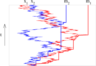
Figure 1: Space-time diagram of the positions (thin lines) and the ordered maxima (thick lines) of two Brownian particles.

The two maxima remain ordered if and only if $m_{1}(\tau)>x_{2}(\tau)$ at all times $0\leq\tau\leq t$. Hence, to find $P$, there is no need to keep track of the maximum $m_{2}$, and it suffices to consider only the position $x_{2}$. As a further simplification, we focus on the distance of each particle from the maximum $m_{1}$ and introduce the variables

$$u=m_{1}-x_{1}\qquad{\rm and}\qquad v=m_{1}-x_{2}.$$ (2)

By definition, both distances are positive, $u\geq 0$ and $v\geq 0$. The transformation (2) maps the four variables (two positions and two maxima) onto the two relevant variables (two distances). Since the positions $x_{1}$ and $x_{2}$ undergo simple diffusion, the distances $u$ and $v$ also undergo simple diffusion in the domain $u>0$ and $v>0$. Hence, the probability density $\rho(u,v,t)$ obeys the diffusion equation $\partial_{t}\rho=D\nabla^{2}\rho$ with $\nabla^{2}=\partial^{2}_{u}+\partial^{2}_{v}$ along with the boundary conditions $\rho\big{|}_{v=0}=0$ and $(\partial_{u}-\partial_{v})\rho\big{|}_{u=0}=0$. The boundary $v=0$ is absorbing so that position $x_{2}$ does not exceed maximum $m_{1}$. The second boundary condition (see Supplemental Material for derivation) is more subtle, and it effectively implies upward drift along the boundary $u=0$: When the maximum increases, $m_{1}\to m_{1}+\delta m$, one distance remains the same, $u=0$, but the second distance increases, $v\to v+\delta m$ (Fig. 2).

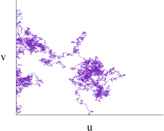
Figure 2: Sample trajectory of the composite particle. There is upward drift along the boundary $u=0$ and the boundary $v=0$ is absorbing.

The probability $P(t)$ is the integral of the probability density, $P(t)=\int_{0}^{\infty}\int_{0}^{\infty}du\,dv\,\rho(u,v,t)$. This quantity equals the survival probability of a “composite” particle with coordinates $(u,v)$ that is undergoing Brownian motion in two dimensions. This composite particle starts somewhere along the boundary $u=0$, and it diffuses in the domain $u>0$ and $v>0$. The particle experiences drift along the boundary $u=0$ but it is annihilated when it reaches the boundary $v=0$ (Figure 2).

In general, the probability $P$ depends on the initial coordinates $u(0)$ and $v(0)$. It is convenient to compute the probability $P$ directly rather than through the probability density $\rho(u,v,t)$. With the shorthand notations $X\equiv u(0)$ and $Y\equiv v(0)$, the probability $P\equiv P(X,Y,t)$ obeys the standard diffusion equation ghw ; bk-mult

$$\frac{\partial P}{\partial t}=D\nabla^{2}P$$ (3)

with the Laplace operator $\nabla^{2}=\partial^{2}_{X}+\partial^{2}_{Y}$. The initial condition is $P=1$ in the region $X\geq 0$ and $Y>0$, and the boundary conditions are $P\big{|}_{Y=0}=0$ and $(\partial_{X}+\partial_{Y})P\big{|}_{X=0}=0$. The former reflects that the boundary $Y=0$ is absorbing, and the second is a consequence of the drift (see Supplemental Material for details). Our problem corresponds to the special case $X=0$ and $Y=x_{1}(0)-x_{2}(0)$.

In terms of the polar coordinates $R=\sqrt{X^{2}+Y^{2}}$ and $\theta=\arctan(Y/X)$, the probability $P\equiv P(R,\theta,t)$ obeys the diffusion equation (3) with the Laplace operator

$$\nabla^{2}=\frac{\partial^{2}}{\partial R^{2}}+\frac{1}{R}\frac{\partial}{\partial R}+\frac{1}{R^{2}}\frac{\partial^{2}}{\partial\theta^{2}}$$

The first boundary condition is simply $P\big{|}_{\theta=0}=0$. The second boundary condition becomes

$$\left(R\,\frac{\partial P}{\partial R}-\frac{\partial P}{\partial\theta}\right)\,\Big{|}_{\theta=\pi/2}=0$$ (4)

where we have utilized $\partial_{X}=\cos\theta\,\partial_{R}-R^{-1}\sin\theta\,\partial_{\theta}$ and $\partial_{Y}=\sin\theta\,\partial_{R}+R^{-1}\cos\theta\,\partial_{\theta}$.

In the long-time limit, the solution to (3) has a separable form bk-mult

$$P(R,\theta,t)\sim\left(\frac{R^{2}}{Dt}\right)^{\beta}\sin\big{(}2\beta\theta\big{)}.$$ (5)

This form can be conveniently obtained using dimensional analysis: the probability $P$ is dimensionless and the quantity $R^{2}/(Dt)$ is the only dimensionless combination of the variables $R,D,t$. Hence, we anticipate $P(R,\theta,t)\sim(R^{2}/Dt)^{\beta}f(\theta)$. Plugging this expression into (3) we see that the left-hand side vanishes in the long-time limit, and the function $f$ obeys $f^{\prime\prime}+(2\beta)^{2}f=0$. We choose $f(\theta)=\sin\left(2\beta\theta\right)$ to satisfy the boundary condition $S\big{|}_{\theta=0}=0$. Next, we substitute (5) into (4), and observe that the second boundary condition is obeyed when $\tan(\beta\pi)=1$. Thus $\beta=1/4$ and we arrive at the slow kinetics (Fig. 3)

$$P\sim t^{-1/4}.$$ (6)

Importantly, the decay exponent is an eigenvalue of the angular component of the Laplace operator, and it is specified by the boundary conditions. We note that the behavior (6) also characterizes the probability that a particle diffusing on a plane avoids a semi-infinite needle cr .

Consider now the general case where the two particles have diffusion constants $D_{1}$ and $D_{2}$. The transformation $(x_{1},x_{2})\to(\widehat{x}_{1},\widehat{x}_{2})$ with $(\widehat{x}_{1},\widehat{x}_{2})=(x_{1}/\sqrt{D_{1}},x_{2}/\sqrt{D_{2}})$ maps this anisotropic Brownian motion onto isotropic Brownian motion in two dimensions. The maxima are also rescaled, $(m_{1},m_{2})\to(\widehat{m}_{1},\widehat{m}_{2})$ with $(\widehat{m}_{1},\widehat{m}_{2})=(m_{1}/\sqrt{D_{1}},m_{2}/\sqrt{D_{2}})$. The two maxima remain ordered, $m_{1}>m_{2}$, as long as

$$\sigma\,\widehat{m}_{1}>\widehat{m}_{2}\qquad\text{with}\qquad\sigma=\sqrt{D_{1}/D_{2}}.$$ (7)

Thus, we expect that the exponent depends on the ratio of diffusion constants, $\beta\equiv\beta(D_{1}/D_{2})$. When one particle is immobile, the problem simplifies. If $D_{1}=0$, the maxima remain ordered if the particles do not meet, $x_{1}(0)>x_{2}(t)$, and hence $P\sim t^{-1/2}$. In the complementary case $D_{2}=0$, an immobile particle can not overtake a maximum set by an mobile particle and $P=1$. The limiting values are therefore $\beta(0)=1/2$ and $\beta(\infty)=0$, and since the exponent should be a monotonic function of the ratio $D_{1}/D_{2}$, we deduce $0\leq\beta\leq 1/2$.

The above analysis is straightforward to generalize if instead of (2) we use the distances $u=\widehat{m}_{1}-\widehat{x}_{1}$ and $v=\sigma\,\widehat{m}_{1}-\widehat{x}_{2}$. Again, diffusion takes place in the domain $u>0$ and $v>0$, and the boundary conditions are $P|_{Y=0}=0$ and $(\partial_{X}+\sigma\,\partial_{Y})P\big{|}_{X=0}=0$. In polar coordinates, the latter boundary condition reads $(\sigma\,R\,\partial_{R}-\partial_{\theta})S\big{|}_{\theta=\pi/2}=0$. Using this boundary condition and the probability $P$ given by (5) we deduce $\sigma\tan\big{(}\beta\pi\big{)}=1$ and thus obtain our main result (1).

The exponent is rational for special values of the diffusion constants, for instance, $\beta(1/3)=1/3$, $\beta(1)=1/4$, and $\beta(3)=1/6$. Exponent $\beta$ varies continuously with the ratio $D_{1}/D_{2}$ (Fig. 4). Unlike the universal first-passage behavior $t^{-1/2}$ characterizing positions of Brownian particles, the behavior of the probability $P$ is not universal and further, it can not be derived using heuristic scaling arguments. Further, first-passage kinetics of maxima of mobile Brownian particles are generally slower compared with first-passage kinetics of positions since $\beta<1/2$. As expected, the limiting values are $\beta(0)=1/2$ and $\beta(\infty)=0$, and further, the limiting behaviors are $1/2-\beta\simeq\tfrac{1}{\pi}\sqrt{D_{1}/D_{2}}$ when $D_{1}\ll D_{2}$ and $\beta\simeq\tfrac{1}{\pi}\,\sqrt{D_{2}/D_{1}}$ for $D_{2}\ll D_{1}$.

Figure 3: The probability $P$ versus time $t$. Shown are Monte Carlo simulation results, obtained from $10^{8}$ independent realizations (circles). Also shown as reference (line) is the theoretical prediction (6).

One anticipates that the asymptotic behavior (1) applies to a broad class of diffusion processes. As a test, we performed Monte Carlo simulations (see also refs. pg ; obdkgs ) of discrete-time random walks in one dimension with two different implementations: (i) a random walk on a lattice where all step lengths have the same size, and (ii) a random walk on a line where the step lengths are chosen from a uniform distribution with compact support. In both cases, the simulation results are in excellent agreement with the theoretical predictions. The simulation results shown in Figures 3 and 4 correspond to random walks on a line.

For $n$ particles undergoing Brownian motion, there are three natural generalizations of the probability $P$. First is the probability $A_{n}$ that all $n$ maxima remain perfectly ordered, that is, $n$ staircases as in Figure 1 never intersect; for positions of Brownian particles, this problem dates back to mef . Second is the probability $B_{n}$ that rightmost staircase is never overtaken, the corresponding problem for positions was studied in bg . Third is the probability $C_{n}$ that the leftmost staircase never overtakes another maxima bjmkr . We expect all three quantities to decay as power laws,

$$A_{n}\sim t^{-\alpha_{n}},\quad B_{n}\sim t^{-\beta_{n}},\quad C_{n}\sim t^{-\gamma_{n}},$$ (8)

with exponents $\alpha_{n}$, $\beta_{n}$, and $\gamma_{n}$ that depend on the number of particles $n$. Table I lists results of Monte Carlo simulations along with the analogous exponents for the positions, rather than the maxima bk-mult .

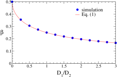
Figure 4: The exponent $\beta$ versus the ratio $D_{1}/D_{2}$. The line corresponds to the theoretical curve (1), and the dots to results of Monte Carlo simulations with $10^{7}$ independent realizations.

	maxima			positions
$n$	$\alpha_{n}$	$\beta_{n}$	$\gamma_{n}$	$a_{n}$	$b_{n}$	$c_{n}$
$3$	$0.653$	$0.432$	$0.335$	$3/2$	$3/4$	$3/8$
$4$	$1.13$	$0.570$	$0.376$	$3$	$0.91$	$0.306$
$5$	$1.60$	$0.674$	$0.401$	$5$	$1.02$	$0.265$
$6$	$2.01$	$0.759$	$0.417$	$15/2$	$1.11$	$0.234$

Table 1: The exponents $\alpha_{n}$, $\beta_{n}$, and $\gamma_{n}$ defined in equation (8) versus the number of particles $n$. Also shown as a reference are values for the corresponding exponents $a_{n}$, $b_{n}$, and $c_{n}$ characterizing analogous probabilities involving the positions of $n$ Brownian particles bk-mult . The only known mef sequence of exponents is $a_{n}=n(n-1)/4$.

All of the exponents are directly related to eigenvalues of the Laplace operator in high-dimensional space with suitable boundary conditions. Even for the simpler case of ordered positions, such eigenvalues are generally unknown (Table I). We expect that $\alpha_{n}>\beta_{n}>\gamma_{n}$ and furthermore that all three exponents increase with $n$. Further, it is possible to justify the behavior $\beta_{n}\simeq b_{n}$ and consequently bk-mult ; bjmkr obtain the logarithmic growth $\beta_{n}\simeq\tfrac{1}{4}\ln n$ when the number of particles is large, $n\to\infty$. Also, it is simple to show that $\gamma_{n}\to 1/2$ in the limit $n\to\infty$ bk14 . Based on the numerical results we conjecture that one of the exponents is rational, $\gamma_{n}=\tfrac{n-1}{2n}$; this form is consistent with $\gamma_{1}=0$ and $\gamma_{2}=1/4$.

Our results thus far concern diffusion in one spatial dimension, yet closely related questions can be asked of Brownian motion in arbitrary dimension $d$. Consider, for example, the maximum distance traveled by a Brownian particle. If the particle starts at the origin, this distance equals the radial coordinate in a spherical coordinate system. We expect that the probability $U_{d}$ that the maximal radial coordinate of one particle always exceeds that of another particle decays algebraically with time, $U_{d}\sim t^{-\nu_{d}}$. Our numerical simulations show that exponent $\nu$ grows rather slowly with dimension $d$

$$\nu_{1}=0.563,\qquad\nu_{2}=0.602,\qquad\nu_{3}=0.630.$$ (9)

It would also be interesting to study planar Brownian excursions and in particular the probability that the convex hull generated by one particle always contains that of a second particle bd ; mcr .

We also mention that the first-passage process studied in this letter is equivalent to a “competition” between two records abn . As a data analysis tool, the first-passage probability $P$ is a straightforward measure and can be used in finance bp , climate nmt ; whk , and earthquakes sdt ; bk13 . The notion of competing maxima could also describe the span of colloidal particles undergoing simple or anomalous diffusion csg ; lkb .

In summary, we studied maxima of Brownian particles in one dimension and found that the probability that such maxima remain ordered decays as a power law with time. The exponent characterizing this decay varies continuously with the diffusion coefficients governing the motion of the particles. When there are two particles, the problem reduces to diffusion in two dimensions with mixed boundary conditions. Recent studies show that the eigenvalues characterizing ordering of a very large number Brownian trajectories obey scaling laws in the thermodynamic limit bk-mult and an interesting open challenge would be to use such scaling methods to elucidate extreme value statistics of many Brownian trajectories.

We acknowledge DOE grant DE-AC52-06NA25396 for support (EB).

Appendix A Supplemental Material

To derive the various boundary conditions, we consider two discrete time random walks. We implement the random walk process as follows: in each time step one of the random walks is chosen at random and it jumps left or right with equal probabilities. Therefore, the coordinates $x$ and $y$ evolve according to

$$(x,y)\to\begin{cases}(x+1,y)&{\rm with\ prob.\ }1/4;\\ (x-1,y)&{\rm with\ prob.\ }1/4;\\ (x,y+1)&{\rm with\ prob.\ }1/4;\\ (x,y-1)&{\rm with\ prob.\ }1/4.\end{cases}$$ (10)

Consequently, the distances $u$ and $v$ change as follows

$$(u,v)\to\begin{cases}(u+1,v)&{\rm with\ prob.\ }1/4,\\ (u-1,v)&{\rm with\ prob.\ }1/4,\\ (u,v+1)&{\rm with\ prob.\ }1/4,\\ (u,v-1)&{\rm with\ prob.\ }1/4,\end{cases}$$ (11)

when $u>0$ and $v>0$. To derive the diffusion equation $\partial_{t}\rho=D\nabla^{2}\rho$ with $D=1/4$ we write the recursion equation

$$\rho(u,v,t+1)=\frac{\rho(u+1,v,t)+\rho(u-1,v,t)+\rho(u,v+1)+P(u,v-1,t)}{4}.$$ (12)

We now expand the left-hand as a first-order Taylor expansion in time and the right-hand side as a second-order Taylor series in space. The diffusion equation is subject to the boundary conditions

$$\left(\frac{\partial\rho}{\partial u}-\frac{\partial\rho}{\partial v}\right)\Big{|}_{u=0}=0\qquad\text{and}\qquad\rho\big{|}_{v=0}=0.$$ (13)

These boundary conditions follow from the jump rules along the lines $u=0$ and $v=0$ respectively,

$$(0,v)\to\begin{cases}(0,v+1)&{\rm with\ prob.\ }1/2;\\ (0,v-1)&{\rm with\ prob.\ }1/4;\\ (1,v)&{\rm with\ prob.\ }1/4.\end{cases}\qquad\text{and}\qquad(u,0)\to\begin{cases}(u+1,0)&{\rm with\ prob.\ }1/4;\\ (u-1,0)&{\rm with\ prob.\ }1/4;\\ (u,1)&{\rm with\ prob.\ }1/4.\end{cases}$$ (14)

In the second case, with probability $1/4$, the second random random walk tries to overtake the maximum set by the first walker and thus, it is annihilated (absorbed by the boundary $v=0$).

As function of the initial coordinates $X$ and $Y$, the probability $P(X,Y,t)$ satisfies a recursion equation analogous to (12)

$$P(X,Y,t+1)=\frac{P(X+1,Y,t)+P(X-1,Y,t)+P(X,Y+1,t)+P(X,Y-1,t)}{4},$$ (15)

leading to the diffusion equation for $P$ with $D=1/4$. The boundary condition $(\partial P/\partial X+\partial P/\partial Y)\big{|}_{X=0}=0$ follows from the recursion

$$P(0,Y,t+1)=\frac{P(1,Y,t)+P(0,Y-1,t)+2P(0,Y+1,t)}{4}.$$ (16)

To derive this equation, we have to take into account all relevant initial conditions $(m_{0},x_{0},y_{0})$ where $m_{0}$ is the initial maximum. The first term corresponds to $(x_{0}+1,x_{0},y_{0})$, the second to $(x_{0},x_{0},y_{0}+1)$, and the third includes contributions from two initial conditions: $(x_{0},x_{0},y_{0}-1)$ and $(x_{0}+1,x_{0}+1,y_{0})$. Of course, we are interested in the behavior along the line $X=0$ which corresponds to $m_{0}=x_{0}$, but the problem is well defined for all $m_{0}\geq x_{0}\geq y_{0}$, a region which lies entirely inside the first quadrant ($X\geq 0$ and $Y\geq 0$) in the $X$-$Y$ plane. Finally, we stress that in our reduced two-variable description, we “integrate” over the initial maximum $m_{0}$.

References

- (1) P. Mörders and Y. Peres, Brownian Motion (Cambridge University Press, Cambridge, 2010).
- (2) E. Sparre Andersen, Math. Scand. 1, 263 (1953); ibid. 2, 195 (1954).
- (3) W. Feller, An Introduction to Probability Theory and Its Applications (Wiley, New York, 1968).
- (4) S. Redner, A Guide to First-Passage Processes (Cambridge University Press, Cambridge, 2001).
- (5) P. Lévy, Processus Stochastiques et Mouvement Brownien (Gauthier-Villars, Paris, 1948).
- (6) K. Itô and H. P. McKean, Diffusion Processes and Their Sample Paths (New York, Springer, 1965).
- (7) S. N. Majumdar, C. Sire, A. J. Bray, and S. J. Cornell, Phys. Rev. Lett. 77, 2867 (1996).
- (8) B. Derrida, V. Hakim, R. Zeitak, Phys. Rev. Lett. 77, 2871 (1996).
- (9) Y. Takikawa and H. Orihara, Phys. Rev. E 88, 062111 (2013).
- (10) G. Coupier, M. Saint Jean, C. Guthmann, EPL 77, 60001 (2007).
- (11) E. Ben-Naim and P. L. Krapivsky, Phys. Rev. Lett. 102, 190602 (2009).
- (12) C. Lutz, M. Kollmann, and C. Bechinger, Phys. Rev. Lett. 93, 026001 (2004).
- (13) E. Barkai and R. Silbey, Phys. Rev. Lett. 102, 050602 (2009).
- (14) P. L. Krapivsky, S. Redner, and E. Ben-Naim, A Kinetic View of Statistical Physics (Cambridge University Press, Cambridge, 2010).
- (15) A. J. Bray, S. N. Majumdar, and G. Schehr, Adv. Phys. 62, 225 (2013).
- (16) B. Derrida, J. L. Lebowitz, and E. R. Speer, Phys. Rev. Lett. 15, 150601 (2001).
- (17) G. Schehr, S. N. Majumdar, A. Comtet, and J. Randon-Furling, Phys. Rev. Lett. 101, 150601 (2008).
- (18) S. N. Majumdar and R. M. Ziff, Phys. Rev. Lett. 101, 050601 (2008).
- (19) E. Ben-Naim and P. L. Krapivsky, arXiv:1404.2966.
- (20) G. H. Weiss, Aspects and Applications of the Random Walk (North-Holland, Amsterdam, 1994).
- (21) E. Ben-Naim and P. L. Krapivsky, J. Phys. A 43, 495007 (2010); J. Phys. A 43, 495008 (2010).
- (22) D. Considine and S. Redner, J. Phys. A 22, 1621 (1988).
- (23) P. Grassberger, Computer Phys. Comm. 147, 64 (2002).
- (24) T. Oppelstrup, V. V. Bulatov, A. Donev, M. H. Kalos, G. H. Gilmer, and B. Sadigh, Phys. Rev. E 80, 066701 (2009).
- (25) M. E. Fisher, J. Stat. Phys. 34, 667 (1984); D. A. Huse and M. E. Fisher, Phys. Rev. B 29, 239 (1984).
- (26) M. Bramson and D. Griffeath, in: Random Walks, Brownian Motion, and Interacting Particle Systems: A Festshrift in Honor of Frank Spitzer, eds. R. Durrett and H. Kesten (Birkhäuser, Boston, 1991).
- (27) P. L. Krapivsky and S. Redner, J. Phys. A 29, 5347 (1996); D. ben-Avraham, B. M. Johnson, C. A. Monaco, P. L. Krapivsky, and S. Redner, J. Phys. A 36, 1789 (2003).
- (28) B. Duplantier, in Fractal Geometry and Applications: A Jubilee of Benoît Mandelbrot (M. L. Lapidus and M. van Frankenhuysen, eds.), Proc. Symposia Pure Math. 72, 365 (2004).
- (29) S. N. Majumdar, A. Comtet, and J. Randon-Furling, J. Stat. Phys. 138, 955 (2010).
- (30) B. C. Arnold, N. Balakrishnan and H. N. Nagraja, Records (Wiley-Interscience, 1998).
- (31) J. -P. Bouchaud and M. Potters, Theory of Financial Risk and Derivative Pricing (Cambridge University Press, Cambridge 2003).
- (32) W. I. Newman, B. D. Malamud, and D. L. Turcotte, Phys. Rev. E 82, 066111 (2010).
- (33) G. Wergen, A. Hense, and J. Krug, Climate Dynamics 42, 1275 (2014).
- (34) R. Shcherbakov, J. Davidsen, and K. F. Tiampo, Phys. Rev. E 87, 052811 (2013).
- (35) E. Ben-Naim and P. L. Krapivsky, Phys. Rev. E 88, 022145 (2013); P. W. Miller and E. Ben-Naim, J. Stat. Mech. P10025 (2013).