Decoherence of a quantum system coupled to an XY spin chain: Role of the initial state of the spin chain

Abstract

We study the decoherence of a coupled quantum system consisting of a central spin and its correlated environment described by a general $XY$ spin-chain model. We make it clear that the evolution of the coherence factor sensitively depends on the initial states of the environment spin-chain. Specially, the dynamical evolution of the coherence factor of the central spin is numerically and analytically investigated in both weak and strong coupling cases for different initial states including thermal equilibrium state. In both weak and strong coupling regimes, the decay of the coherence factor can be approximated by a Gaussian and in the strong coupling regime the coherence factor oscillate rapidly under a Gaussian envelope. The width of the Gaussian decay (envelope) has been studied in details and we explained the origin of the so-called universal regime.

Docoherence induced by coupling a quantum system with an environment is one of the most important different features of opened quantum systems from isolated ones. It refers to the process that turns the system from quantum coherent pure states into classical mixed states. Usually, this process will destroy the coherence between the pointer states corresponding to their eigenvalues in a short time Zurek1 and is a major obstacle in quantum information processing (QIP) that use the coherent entangled states as resources Weiss ; Breuer . Hence the study of docoherence is important for understanding quantum physics and the implementation of QIP.

The decoherence process depends on the effective Hamiltonian and the initial state of the environment. The effects of the effective Hamiltonian on the decoherence has been studied in many papers Cormick1 ; Cormick2 ; You ; Cheng ; Lian ; Quan ; Yuan1 ; Yuan2 ; Liu ; Cucc1 ; Cucc2 ; Ai ; Li ; Sun ; Damski ; Cincio . Especially, dramatic manifestation of the decoherence has often been found in the vicinity of the quantum critical point of the effective Hamiltonian. Hence much work have been focused on the critical properties of the decoherence Quan ; Yuan1 ; Cheng ; Ai ; Li ; Sun ; Damski ; Cincio . Whereas, the dependence of the decoherence on the initial state of the environment has been rarely mentioned Win ; Moro and thus will be studied in this paper. In particular, we will focus on the Gaussian decay Cucc1 ; Cucc2 ; Zurek2 ; Cormick1 ; Yuan2 ; Rossini and explain the origin of the so-called universal regime of the Gaussian decay Cucc1 ; Cormick1 .

The dynamical evolution of the reduced density matrix may be used to describe the decoherence process. For a two-level qubit system such as a central spin, which is coupled to an environment of an $XY$ spin chain, the coefficients of the off-diagonal terms in the reduced density matrix of the system, named as “coherence factor” in the following discussion in this paper, may describe the degree of the decoherence. It was found that in such a simple model and with a few additional generic assumptions, the coherence factor displays a Gaussian decay. So the Gaussian decay is general and important for the decoherence research. Furthermore, a universal regime of the Gaussian envelope has been found when the coupling strength is large enough, which means that the envelope of the decay of the coherence factor in the system is Gaussian with a width independent of the system-environment coupling strength Cucc1 ; Cormick1 . While in another case, the Gaussian width in the strong coupling regime may be proportional to the coupling strength Yuan2 .

Now we introduce the Hamiltonian and the model. We consider a two-level quantum system (central spin) transversely coupled to an environment which is described by one-dimensional $XY$ spin chain model. The total Hamiltonian is given by $H$=$H_{E}^{\lambda}$+$H_{I}$, where (we take $\hbar$=$1$)

$$H_{E}^{\lambda} =-\overset{N}{\sum_{l=1}}\left(\frac{1+\gamma}{2}\sigma_{l}^{x}\sigma_{l+1}^{x}+\frac{1-\gamma}{2}\sigma_{l}^{y}\sigma_{l+1}^{y}+\lambda\sigma_{l}^{z}\right),$$ (1)

$$H_{I} =-g\sigma^{z}\overset{N}{\sum_{l=1}}\sigma_{l}^{z}.$$

Here $H_{E}^{\lambda}$ denotes the Hamiltonian of the environmental spin chain and $H_{I}$ denotes the interaction between the central spin and the environment. $\sigma^{\alpha}$ ($\alpha$=$x$, $y$, $z$) and $\sigma_{l}^{\alpha}$ are the Pauli matrices used to describe the central spin and the $j$th spin of the spin chain, respectively. The parameters $\lambda$ characterizes the strength of the spin interaction and the intensity of the magnetic filed applied along the $z$ axis respectively, and $\gamma$ measures the anisotropy in the in-plane interaction. $N$ is the total site number in the spin chain.

Before going any further, we explain how we dress the parameter of the intensity of the magnetic filed $\lambda$ and the Hamiltonian $H_{E}^{\lambda}$ in this paper. To explore the dependence of the decoherence on the initial states of the spin-chain, we should analyze various initial states. A natural and simple choice of the initial state is the ground state of the initial Hamiltonian $H_{E}^{\left(\lambda_{i}\right)}$ at time $t$=$0$ which may be different from the evolving Hamiltonian $H_{E}^{\left(\lambda_{e}\right)}$ for time $t$$>$$0$. Both of the the initial Hamiltonian $H_{E}^{\left(\lambda_{i}\right)}$ and the evolving Hamiltonian $H_{E}^{\left(\lambda_{e}\right)}$ are defined as $H_{E}^{\lambda}$ in Eq. (1) by replacing $\lambda$ with $\lambda_{i}$ and $\lambda_{e}$, respectively. That is, we assume that the coupling between the central system and the environment begin at $t$=$0$ and there may be a sudden change for the intensity $\lambda$ of the Hamiltonian at $t$=$0$. For simplicity, in the following of this paper we use $H$=$H_{E}^{\left(\lambda_{e}\right)}$+$H_{I}$ to represent the total Hamiltonian for $t$$>$$0$. Furthermore, we use $\lambda_{+}$=$\lambda_{e}\mathtt{+}g$ and $\lambda_{-}\mathtt{=}\lambda_{e}\mathtt{-}g$ to dress the intensity of the magnetic filed for two effective Hamiltonians $H_{E}^{\left(\lambda_{+}\right)}$ and $H_{E}^{\left(\lambda_{-}\right)}$, which are defined as $H_{E}^{\lambda}$ in Eq. (1) by replacing $\lambda$ with $\lambda_{+}$ and $\lambda_{-}$, respectively. So in this paper we label the intensity of the magnetic field with four types: $\lambda_{i}$, $\lambda_{e}$, $\lambda_{+}$ and $\lambda_{-}$.

Following Ref. Yuan2 , we can rewrite the total Hamiltonian $H$ as

$$H=\left|0\right\rangle\left\langle 0\right|\otimes H_{E}^{\left(\lambda_{+}\right)}+\left|1\right\rangle\left\langle 1\right|\otimes H_{E}^{\left(\lambda_{-}\right)},$$ (2)

where $\left|0\right\rangle$ and $\left|1\right\rangle$ denote the eigenstates of $\sigma^{z}$ with eigenvalues of $\pm 1$. $H_{E}^{\left(\lambda_{+}\right)}$ and $H_{E}^{\left(\lambda_{-}\right)}$ are the corresponding effective Hamiltonians of the spin chain. $H_{E}^{\left(\lambda_{j}\right)}$($j$=$i,e,+,-$) can be diagonalized by standard procedure Sach . As the first step, we define the conventional Jordan-Wigner (JW) transformation as follows

$$\sigma_{l}^{x} =\underset{m<l}{{\displaystyle\prod}}\left(1-2a_{m}a_{m}^{{\dagger}}\right)\left(a_{l}+a_{l}^{{\dagger}}\right),$$ (3)

$$\sigma_{l}^{y} =-i\underset{m<l}{{\displaystyle\prod}}\left(1-2a_{m}a_{m}^{{\dagger}}\right)\left(a_{l}-a_{l}^{{\dagger}}\right),$$ (4)

$$\sigma_{l}^{z} =1-2a_{l}a_{l}^{{\dagger}},$$ (5)

which maps spins to one-dimensional spinless fermions with creation (annihilation) operators $a_{l}^{{\dagger}}$ ($a_{l}$). After a straightforward derivation, the Hamiltonians become

$$H_{E}^{\left(\lambda_{j}\right)}=-\overset{N}{\sum_{l=1}}\left[\left(a_{l+1}^{{\dagger}}a_{l}+a_{l}^{{\dagger}}a_{l+1}\right)+\gamma\left(a_{l+1}a_{l}+a_{l}^{{\dagger}}a_{l+1}^{{\dagger}}\right)-\lambda_{j}\left(1-2a_{l}^{{\dagger}}a_{l}\right)\right].$$ (6)

In the second step, we introduce the Fourier transformation of the fermionic operators described by $a_{k}$=$\frac{1}{\sqrt{N}}{\textstyle\sum\nolimits_{l}}a_{l}e^{-i2\pi lk/N}$, with $k$=$-M+1,..,M;M=N/2$. The Hamiltonian (6) can be diagonalized by transforming the fermion operators to momentum space and then using the Bogoliubov transformation. The final result is

$$H_{E}^{\left(\lambda_{j}\right)} =\overset{M}{\underset{k=1}{{\displaystyle\sum}}}H_{E}^{\left(k,\lambda_{j}\right)}$$

$$=\overset{M}{\underset{k=1}{{\displaystyle\sum}}}\Omega_{k}^{\left(\lambda_{j}\right)}\left(b_{k,\lambda_{j}}^{{\dagger}}b_{k,\lambda_{j}}-\frac{1}{2}\right),$$ (7)

where $H_{E}^{\left(k,\lambda_{j}\right)}$=$\Omega_{k}^{\left(\lambda_{j}\right)}\left(b_{k,\lambda_{j}}^{{\dagger}}b_{k,\lambda_{j}}-\frac{1}{2}\right)$ and the energy spectrum is given by

$$\Omega_{k}^{\left(\lambda_{j}\right)}=2\sqrt{\left(\epsilon_{k}^{\left(\lambda_{j}\right)}\right)^{2}+\gamma^{2}\sin^{2}\frac{2\pi k}{N}}$$ (8)

with $\epsilon_{k}^{\left(\lambda_{j}\right)}$=$\lambda_{j}-\cos\frac{2\pi k}{N}$, and the correspoding Bogoliubov transformed fermion operators are defined by

$$b_{k,\lambda_{j}}=\cos\frac{\theta_{k}^{\left(\lambda_{j}\right)}}{2}a_{k,\lambda_{j}}-i\sin\frac{\theta_{k}^{\left(\lambda_{j}\right)}}{2}a_{-k,\lambda_{j}}^{{\dagger}}$$ (9)

with angles $\theta_{k}^{\left(\lambda_{j}\right)}$ =$\arccos[2\epsilon_{k}^{\left(\lambda_{j}\right)}/\Omega_{k}^{\left(\lambda_{j}\right)}].$ The corresponding ground state $\left|G\right\rangle_{\lambda_{j}}$ of $H_{E}^{\left(\lambda_{j}\right)}$ is the vacuum of the fermionic modes described by $b_{k,\lambda_{j}}\left|G\right\rangle_{\lambda_{j}}$=$0$ for any $b_{k,\lambda_{j}}$ and can be written as

$$\left|G\right\rangle_{\lambda_{j}}=\prod\nolimits_{k=1}^{M}\left|G\right\rangle_{\lambda_{j}}^{k}={\textstyle\prod\nolimits_{k=1}^{M}}\left[\cos\frac{\theta_{k}^{\left(\lambda_{j}\right)}}{2}\left|0\right\rangle_{k}\left|0\right\rangle_{-k}+i\sin\frac{\theta_{k}^{\left(\lambda_{j}\right)}}{2}\left|1\right\rangle_{k}\left|1\right\rangle_{-k}\right],$$ (10)

where

$$\left|G\right\rangle_{\lambda_{j}}^{k}=\cos\frac{\theta_{k}^{\left(\lambda_{j}\right)}}{2}\left|0\right\rangle_{k}\left|0\right\rangle_{-k}+i\sin\frac{\theta_{k}^{\left(\lambda_{j}\right)}}{2}\left|1\right\rangle_{k}\left|1\right\rangle_{-k},$$ (11)

$\left|0\right\rangle_{k}$ and $\left|1\right\rangle_{k}$ denote the vacuum and single excitation of the $k$th mode $a_{k,\lambda_{j}}$, respectively. It is straightforward to see that the operator $b_{k,\lambda_{j}}$ is related to the operator $b_{k,\lambda_{j^{\prime}}}$ by the following relation:

$$b_{k,\lambda_{j}}=\left[\cos\alpha_{k}^{\left(\lambda_{jj^{\prime}}\right)}\right]b_{k,\lambda_{j^{\prime}}}-i\left[\sin\alpha_{k}^{\left(\lambda_{jj^{\prime}}\right)}\right]b_{-k,\lambda_{j^{\prime}}}^{{\dagger}},$$ (12)

where $j$=$i,e,+,-$, and $\alpha_{k}^{\left(\lambda_{jj^{\prime}}\right)}$=$\frac{\theta_{k}^{\left(\lambda_{j}\right)}-\theta_{k}^{\left(\lambda_{j^{\prime}}\right)}}{2}$. As a result, the corresponding ground states satisfy the relation

$$|G\rangle_{\lambda_{j}}=\prod\nolimits_{k=1}^{M}\left[\cos\alpha_{k}^{\left(\lambda_{jj^{\prime}}\right)}+i\sin\alpha_{k}^{\left(\lambda_{jj^{\prime}}\right)}b_{k,\lambda_{j^{\prime}}}^{{\dagger}}b_{-k,\lambda_{j^{\prime}}}^{{\dagger}}\right]|G\rangle_{\lambda_{j^{\prime}}}.$$ (13)

Suppose the initial state of the total system is described by the density matrix:

$$\rho_{\mathbf{tot}}\left(0\right)=\rho_{s}\left(0\right)\otimes\rho_{E}\left(0\right),$$ (14)

where $\rho_{s}\left(0\right)$ and $\rho_{E}\left(0\right)$ is the initial density matrix of the central system and the environment respectively. The evolved density matrix of the total system for $t>0$ is

$$\rho_{\mathbf{tot}}\left(t\right)=U\left(t\right)\rho_{\mathbf{tot}}\left(0\right)U^{{\dagger}}\left(t\right),$$ (15)

where $U\left(t\right)$ is the time evolution matrix which can be obtained by solving the equation

$$i\dot{U}\left(t\right)=HU.$$

Equation (15) has an exact solution for a time-dependent step function form for the magnetic field $\lambda\left(t\right)=\lambda_{i}+\left(\lambda_{e}-\lambda_{i}\right)\theta\left(t\right)$ which we adopt in this work Sadiek ; Alkur . Here $\theta\left(t\right)$ is the usual mathematical step function. The solution to the time evolution operator for the Hamiltonian of the time-dependent step function form is exactly the same as that for the Hamiltonian of $H$ for $t>0$. That is, the time evolution operator can be expressed as

$$U\left(t\right)=\left|0\right\rangle\left\langle 0\right|\otimes U_{E}^{\left(\lambda_{+}\right)}\left(t\right)+\left|1\right\rangle\left\langle 1\right|\otimes U_{E}^{\left(\lambda_{-}\right)}\left(t\right),$$ (16)

where $U_{E}^{\left(\lambda_{\pm}\right)}\left(t\right)$=$\exp\left[-iH_{E}^{\left(\lambda_{\pm}\right)}t\right]$ is the effective time evolution operator dressed by $\lambda_{\pm}$. As a result, the reduced density matrix of the central system is

$$\rho_{S}\left(t\right) =\mathbf{Tr}_{E}\left[\rho_{\mathbf{tot}}\left(t\right)\right]$$

$$=\left(\begin{array}[c]{cc}\left[\rho_{S}\left(0\right)\right]_{11}&\left[\rho_{S}\left(0\right)\right]_{12}\left[\mathbf{Tr}_{E}U_{E}^{\left(\lambda_{+}\right)}\left(t\right)\rho_{E}\left(0\right)U_{E}^{{\dagger}\left(\lambda_{-}\right)}\left(t\right)\right]\\ \left[\rho_{S}\left(0\right)\right]_{21}\left[\mathbf{Tr}_{E}U_{E}^{\left(\lambda_{-}\right)}\left(t\right)\rho_{E}\left(0\right)U_{E}^{{\dagger}\left(\lambda_{+}\right)}\left(t\right)\right]&\left[\rho_{S}\left(0\right)\right]_{22}\end{array}\right).$$ (19)

It reveals in Eq. (19) that the environmental spin chain only modulates the off-diagonal terms of $\rho\left(t\right)$ through the coherence factor

$$F\left(t\right)=\left|\mathbf{Tr}_{E}\left[U_{E}^{\left(\lambda_{+}\right)}\left(t\right)\rho_{E}\left(0\right)U_{E}^{{\dagger}\left(\lambda_{-}\right)}\left(t\right)\right]\right|,$$ (20)

Equation (20) is our starting point of the following derivation and discussions. If the initial density matrix of the environmental spin chain $\rho_{E}\left(0\right)$ can be factored as $\rho_{E}\left(0\right)$=$\prod\nolimits_{k=1}^{M}\otimes\rho_{E}^{k}\left(0\right)$, then

$$F\left(t\right)=\prod\nolimits_{k=1}^{M}F_{k}\left(t\right),$$ (21)

where

$$F_{k}\left(t\right)=\left|\mathbf{Tr}_{E}\left\{\exp\left[iH_{E}^{\left(k,\lambda_{+}\right)}t\right]\rho_{E}^{k}\left(0\right)\exp\left[-iH_{E}^{\left(k,\lambda_{-}\right)}t\right]\right\}\right|.$$ (22)

Following Refs. Sadiek ; Alkur , we can also rewrite the Hamiltonian $H_{E}^{\left(k,\lambda_{j}\right)}$ and the effective time evolution operator $U_{E}^{\left(k,\lambda_{j}\right)}\left(t\right)$=$\exp\left[-iH_{E}^{\left(k,\lambda_{j}\right)}t\right]$ in the basis of $\left|\phi_{k}\right\rangle_{1}\mathtt{=}\left|0\right\rangle$, $\left|\phi_{k}\right\rangle_{2}\mathtt{=}a_{k,\lambda_{j}}^{{\dagger}}a_{-k,\lambda_{j}}^{{\dagger}}\left|0\right\rangle$, $\left|\phi_{k}\right\rangle_{3}\mathtt{=}a_{k,\lambda_{j}}^{{\dagger}}\left|0\right\rangle$, and $\left|\phi_{k}\right\rangle_{4}=a_{-k,\lambda_{j}}^{{\dagger}}\left|0\right\rangle$ (or equivelently $\left|0\right\rangle_{k}\left|0\right\rangle_{-k}$, $\left|1\right\rangle_{k}\left|1\right\rangle_{-k}$, $\left|1\right\rangle_{k}\left|0\right\rangle_{-k}$, and $\left|0\right\rangle_{k}\left|1\right\rangle_{-k}$) as follows:

$$H_{E}^{\left(k,\lambda_{j}\right)}=\left\{\begin{array}[c]{cccc}-\Omega_{k}^{\left(\lambda_{j}\right)}\cos\theta_{k}^{j}-2\cos\frac{2\pi k}{N}&i\Omega_{k}^{\left(\lambda_{j}\right)}\sin\theta_{k}^{j}&0&0\\ -i\Omega_{k}^{\left(\lambda_{j}\right)}\sin\theta_{k}^{j}&\Omega_{k}^{\left(\lambda_{j}\right)}\cos\theta_{k}^{j}-2\cos\frac{2\pi k}{N}&0&0\\ 0&0&-2\cos\frac{2\pi k}{N}&0\\ 0&0&0&-2\cos\frac{2\pi k}{N}\end{array}\right\},$$ (23)

$$U_{E}^{\left(k,\lambda_{j}\right)}\left(t\right)=e^{2it\cos\phi_{k}}\left\{\begin{array}[c]{cccc}i\cos\theta_{k}^{j}\sin\left(2t\Lambda_{k}^{j}\right)+\cos\left(2t\Lambda_{k}^{j}\right)&\sin\theta_{k}^{j}\sin\left(2t\Lambda_{k}^{j}\right)&0&0\\ -\sin\theta_{k}^{j}\sin\left(2t\Lambda_{k}^{j}\right)&-i\cos\theta_{k}^{j}\sin\left(2t\Lambda_{k}^{j}\right)+\cos\left(2t\Lambda_{k}^{j}\right)&0&0\\ 0&0&1&0\\ 0&0&0&1\end{array}\right\}.$$ (24)

Then for specific initial state of the environmental system $\rho_{E}\left(0\right)$, we can derive the corresponding coherence factor $F\left(t\right)$.

A natural choice of the initial state of the environmental system is the ground state $\left|G\right\rangle_{\lambda_{i}}$ of the initial Hamiltonian $H_{E}^{\left(k,\lambda_{i}\right)}$,

$$\rho_{k}\left(0\right)=S^{{\dagger}}\left(\begin{array}[c]{cccc}1&0&0&0\\ 0&0&0&0\\ 0&0&0&0\\ 0&0&0&0\end{array}\right)S=\left(\begin{array}[c]{cccc}\frac{1}{2}+\frac{1}{2}\cos\theta_{k}^{i}&-\frac{i}{2}\sin\theta_{k}^{i}&0&0\\ \frac{i}{2}\sin\theta_{k}^{i}&\frac{1}{2}-\frac{1}{2}\cos\theta_{k}^{i}&0&0\\ 0&0&0&0\\ 0&0&0&0\end{array}\right),$$ (25)

where

$$S=\left(\begin{array}[c]{cccc}\cos\frac{\theta_{k}^{i}}{2}&-i\sin\frac{\theta_{k}^{i}}{2}&0&0\\ -i\sin\frac{\theta_{k}^{i}}{2}&\cos\frac{\theta_{k}^{i}}{2}&0&0\\ 0&0&1&0\\ 0&0&0&1\end{array}\right)$$

is the transformation matrix. Then we can get the coherence factor $F\left(t\right)$ with the Eq. (22). The result is

$$F\left(t\right) =\prod\nolimits_{k=1}^{M}|[\cos 2\alpha_{k}^{\left(\lambda_{+-}\right)}\sin\left(\Omega_{k}^{\left(\lambda_{+}\right)}t\right)\sin\left(\Omega_{k}^{\left(\lambda_{-}\right)}t\right)+\cos\left(\Omega_{k}^{\left(\lambda_{+}\right)}t\right)\cos\left(\Omega_{k}^{\left(\lambda_{-}\right)}t\right)$$

$$+i\cos 2\alpha_{k}^{\left(\lambda_{+i}\right)}\sin\left(\Omega_{k}^{\left(\lambda_{+}\right)}t\right)\cos\left(\Omega_{k}^{\left(\lambda_{-}\right)}t\right)-i\cos 2\alpha_{k}^{\left(\lambda_{-i}\right)}\sin\left(\Omega_{k}^{\left(\lambda_{+}\right)}t\right)\cos\left(\Omega_{k}^{\left(\lambda_{-}\right)}t\right)]|,$$ (26)

or equivalently

$$F\left(t\right) =\prod\nolimits_{k=1}^{M}|-\exp\left[it\left(\Omega_{k}^{\left(\lambda_{+}\right)}+\Omega_{k}^{\left(\lambda_{-}\right)}\right)\right]\sin\alpha_{k}^{\left(\lambda_{+-}\right)}\cos\alpha_{k}^{\left(\lambda_{+i}\right)}\sin\alpha_{k}^{\left(\lambda_{-i}\right)}$$

$$+\exp\left[it\left(-\Omega_{k}^{\left(\lambda_{+}\right)}+\Omega_{k}^{\left(\lambda_{-}\right)}\right)\right]\cos\alpha_{k}^{\left(\lambda_{+-}\right)}\sin\alpha_{k}^{\left(\lambda_{+i}\right)}\sin\alpha_{k}^{\left(\lambda_{-i}\right)}$$

$$+\exp\left[it\left(\Omega_{k}^{\left(\lambda_{+}\right)}-\Omega_{k}^{\left(\lambda_{-}\right)}\right)\right]\cos\alpha_{k}^{\left(\lambda_{+-}\right)}\cos\alpha_{k}^{\left(\lambda_{+i}\right)}\cos\alpha_{k}^{\left(\lambda_{-i}\right)}$$

$$+\exp\left[it\left(-\Omega_{k}^{\left(\lambda_{+}\right)}-\Omega_{k}^{\left(\lambda_{-}\right)}\right)\right]\sin\alpha_{k}^{\left(\lambda_{+-}\right)}\sin\alpha_{k}^{\left(\lambda_{+i}\right)}\cos\alpha_{k}^{\left(\lambda_{-i}\right)}|.$$ (27)

In Refs. Quan ; Yuan1 ; Yuan2 , it has been shown that the coherence factor $F\left(t\right)$ decay more dramatically and rapidly in the vicinity of the quantum critical point $\lambda_{i}$=$\lambda_{e}$=$1$.$0$ Quan ; Yuan1 ; Yuan2 for small $N$ ($N\mathtt{\approx}10^{2}$). In this paper we will study the decoherence with different initial states. Hence in Fig. 1 we show dynamical evolution of the coherence facotor $F\left(t\right)$ as a function of time $t$ and $\lambda_{i}$ and keep $\lambda_{e}$=$1$ here and in the following unless specified. The other parameters are $\gamma$=$1$, $g$=$0.05$, $N$=$10^{2}$. One can see that $F\left(t\right)$ with any $\lambda_{i}$ decays from unity to zero in a short time. And around $\lambda_{i}$=$1$, there are significant revivals. This indicates that the decoherence process with different $\lambda_{i}$ and fixed $\lambda_{e}$ may include new interesting behavior and lead to more results.

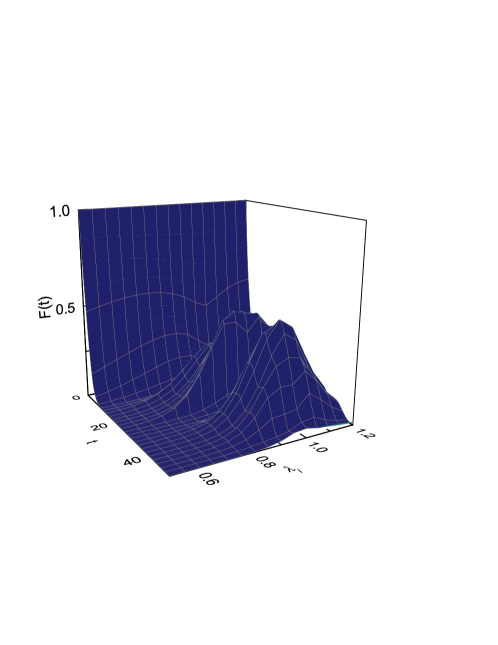
Figure 1: (Color online). The coherence factor $F\left(t\right)$ as a function of time $t$ and $\lambda_{i}$ for Ising ($\gamma$=$1$) spin chain with a size of $N$=$100$.

In fact, the revivals only appear for small $N$. For large $N$ which may be used to simulate the thermodynamic limit, there are no revivals. In Fig. 2 we show the evolution of $F\left(t\right)$ as a function of time $t$ and $\lambda_{i}$. The other parameters are $\gamma$=$1$, $g$=$0.05$, and $N$=$10^{4}$. One can see that $F\left(t\right)$ decays rapidly with no revivals for any $\lambda_{i}$. The disappearance of the revivals for large $N$ can be understood in the following way. Notice that $F\left(t\right)$ is a product of a series of $k$ modes. At $t$=$0$, the module of every mode is unity. After that, some of them decays remarkably, and the others remain unity. The rapid decay is induced by the effect of QPT of the evolving Hamiltonian $\lambda_{e}$=$1$. The effect of QPT come down to the disappearance of the energy gap between the ground state and the excited states. For small $N$, the number of the modes whose energy gaps nearly disappear is small. As a result, the evolution of the coherence factor $F\left(t\right)$ depends on the evolution of $F_{k}\left(t\right)$ of few modes. Hence there are revivals. For large $N$, the number of the modes whose energy gaps nearly disappear is large and thus leads to a chaos result with no revivals.

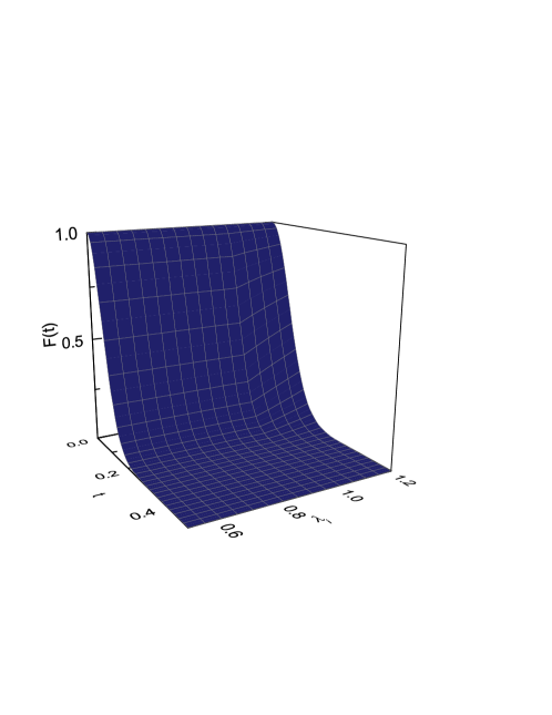
Figure 2: (Color online). The coherence factor $F\left(t\right)$ as a function of time $t$ and $\lambda_{i}$ for Ising ($\gamma$=$1$) spin chain with a size of $N$=$1\times 10^{4}$.

In fact, the decay of the coherence factor $F\left(t\right)$ is Gaussian. The Gaussian decay arises from the following expression

$$r(t) =\overset{M}{\underset{k}{{\displaystyle\prod}}}r_{k}(t)$$ (28)

$$=\overset{M}{\underset{k}{{\displaystyle\prod}}}\left[\left|\alpha_{k}\right|^{2}\exp\left(i\Omega_{k}t\right)+\left|\beta_{k}\right|^{2}\exp\left(-i\Omega_{k}t\right)\right],$$ (29)

where the coefficients $\left|\alpha_{k}\right|^{2}$ and $\left|\beta_{k}\right|^{2}$ satisfy $\left|\alpha_{k}\right|^{2}$+$\left|\beta_{k}\right|^{2}$=$1$. The value of such an expression can be understood as the “random walk” problem discussed in Refs. Cucc1 ; Cucc2 , in which the authors considered the distribution of $M$-step random walk. Each step correlates to a random variable taking the value $+\Omega_{k}$ or $-\Omega_{k}$ with probability $\left|\alpha_{k}\right|^{2}$ or $\left|\beta_{k}\right|^{2}$ respectively. We denote $a_{k}$ and $b_{k}$ the mean value and its variance of the random variable. If Lindeberg condition, which demands that the cumulative variances is finite, is satisfied, this distribution of energies yields a approximately Gaussian time dependence of $r(t)$ as

$$|r(t)|\approx\exp\left(-\frac{s_{M}^{2}t^{2}}{2}\right),$$ (30)

where

$$s_{M}^{2}=\underset{k}{\overset{M}{{\displaystyle\sum}}}b_{k}^{2}$$ (31)

is the cumulative variance.

In the expression of the coherence factor for $\left|G\right\rangle_{\lambda_{i}}$, Eq. (27), $F_{k}$ has four terms. While the sum of the coefficients of the four terms is still unity. This enlightens us to consider $M$-step random walk with random varible taking the values $\Omega_{k1}$=$+\left(\Omega_{k}^{\left(\lambda_{+}\right)}+\Omega_{k}^{\left(\lambda_{-}\right)}\right)$, $\Omega_{k2}$=$-\left(\Omega_{k}^{\left(\lambda_{+}\right)}+\Omega_{k}^{\left(\lambda_{-}\right)}\right)$, $\Omega_{k3}$=$+\left(\Omega_{k}^{\left(\lambda_{+}\right)}-\Omega_{k}^{\left(\lambda_{-}\right)}\right)$, and $\Omega_{k4}$=$-\left(\Omega_{k}^{\left(\lambda_{+}\right)}-\Omega_{k}^{\left(\lambda_{-}\right)}\right)$ with “probabilities” $p_{k1}$=$\sin\alpha_{k}^{\left(\lambda_{+-}\right)}\cos\alpha_{k}^{\left(\lambda_{+i}\right)}\sin\alpha_{k}^{\left(\lambda_{-i}\right)}$, $p_{k2}$=$\cos\alpha_{k}^{\left(\lambda_{+-}\right)}\sin\alpha_{k}^{\left(\lambda_{+i}\right)}\sin\alpha_{k}^{\left(\lambda_{-i}\right)}$, $p_{k3}$=$\cos\alpha_{k}^{\left(\lambda_{+-}\right)}\cos\alpha_{k}^{\left(\lambda_{+i}\right)}\cos\alpha_{k}^{\left(\lambda_{-i}\right)}$, and $p_{k4}$=$\sin\alpha_{k}^{\left(\lambda_{+-}\right)}\sin\alpha_{k}^{\left(\lambda_{+i}\right)}\cos\alpha_{k}^{\left(\lambda_{-i}\right)}$, respectively. Although the “probability” may be negative, the derivation process is similar with that given in Refs. Cucc1 ; Cucc2 . For this purpose we define $a_{k}$=$\bar{\Omega}_{kl}$=${\textstyle\sum\nolimits_{l=1}^{4}}p_{kl}\Omega_{kl}$ and $b_{k}$=${\textstyle\sum\nolimits_{l=1}^{4}}\left(p_{kl}\Omega_{kl}^{2}-p_{kl}a_{k}^{2}\right)$ as mean value and variance of the four random variables, respectively. After a straightforward derivation, we get, in the case of the initial state being $\left|G\right\rangle_{\lambda_{i}}$,

$$a_{k} =4g\cos\theta_{k}^{i},$$ (32)

$$s_{M}^{2} =\underset{k}{\overset{M}{{\displaystyle\sum}}}b_{k}^{2}=\underset{k}{\sum}\underset{l}{\sum}\left[p_{kl}\left(\Omega_{kl}-a_{k}\right)^{2}\right]=16g^{2}\underset{k}{\sum}\sin^{2}\theta_{k}^{i}.$$ (33)

For large $N$, the Lindeberg condition is satisfied and the decoherence factor is

$$F(t)\approx\exp\left(-s_{M}^{2}t^{2}/2\right)\approx\exp\left(-8g^{2}t^{2}\underset{k}{\sum}\sin^{2}\theta_{k}^{i}\right).$$ (34)

By noting that for $\gamma$=$1$,

$$\underset{k}{\sum}\sin^{2}\theta_{k}^{i}\approx\left\{\begin{array}[c]{c}\frac{M}{2\lambda_{i}^{2}}\\ \frac{M}{2}\end{array}\right.\begin{array}[c]{c}\lambda_{i}^{2}>1\\ \lambda_{i}^{2}\leq 1\end{array},$$ (35)

we get

$$s_{M}^{2}\approx\left\{\begin{array}[c]{c}\frac{8g^{2}M}{\lambda_{i}^{2}}\\ 8g^{2}M\end{array}\right.\begin{array}[c]{c}\lambda_{i}^{2}>1\\ \lambda_{i}^{2}\leq 1\end{array}.$$ (36)

Thus, the evolution of coherence factor $F(t)$ of Ising model ($\gamma$=$1$) can be approximated by a very simple formula,

$$F\left(t\right)\approx\left\{\begin{array}[c]{c}\exp\left(-4Mg^{2}t^{2}/\lambda_{i}^{2}\right)\\ \exp\left(-4Mg^{2}t^{2}\right)\end{array}\right.\begin{array}[c]{c}\lambda_{i}^{2}>1\\ \lambda_{i}^{2}\leq 1\end{array},$$ (37)

which is only affected by the coupling strength $g$, $M$ and $\lambda_{i}$. With certain $\lambda_{i}$, bigger chain number and stronger coupling strength, $F(t)$ will decay more rapidly. In the previous work Cormick1 ; Mukh , the relation between the width of the Gaussian decay and the parameters of the Hamiltonian has been studied. Here we first give the expression for the reciprocal of the width $s_{M}^{2}$ with the parameters of the Hamiltonian for Ising ($\gamma$=$1$) model. In Fig. 3 we show the numerical results of $F(t)$ as a function of $t$ with $\lambda_{i}$=$0.5$ and $\lambda_{i}$=$1.5$ respectively. These results are calculated with Eqs. (27), (34), and (37) respectively. The solid lines are drawn with Eq. (27); the dash lines are drawn with Eq. (34); the dot lines are drawn with E.q. (37). The three upper lines are drawn with $\lambda_{i}$=$0.5$ and the lower lines are drawn with $\lambda_{i}$=$1.5$. One can see that the lines from either Eq. (34) or (37) fit the lines from Eq. (27) very well. From Eq. (36) one can also see that the critical point ($\lambda_{i}$=$1$) of the initial Hamiltonian still plays a special role. At this critical point, the decaying speed is not particularly high, while the derivative of $s_{M}^{2}$ with $\lambda_{i}^{2}$ becomes discontinuous.

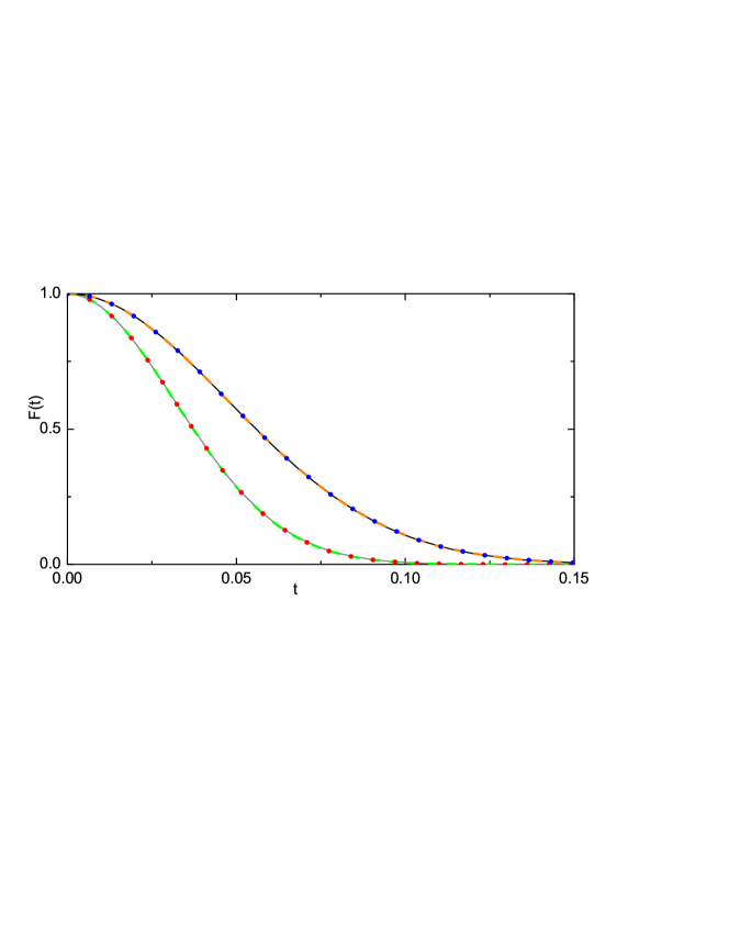
Figure 3: (Color online). The evolution of the coherence factor $F\left(t\right)$ and its approximate analytic expressions Eqs. (34) and (37) as a function of time $t$ with $\lambda_{i}$=$0.5$ and $\lambda_{i}$=$1.5$ for Ising ($\gamma$=$1$) spin chain with a size of $N$=$10^{5}$. Here, the solid lines are drawn with Eq. (27), the dash lines are drawn with Eq. (34), and the dot lines are drawn with Eq. (37).

Next, we choose thermal equilibrium state as initial state. By noting that the partition function of the thermal equilibrium state should be determined by the initial Hamiltonian $H_{E}^{\left(\lambda_{i}\right)}$, but not $H_{E}^{\left(\lambda_{e}\right)}$, we can derive the expression for the coherence factor as

$$F\left(t\right) =\frac{1}{Z}|[\cos 2\alpha_{k}^{\left(\lambda_{+-}\right)}\sin\left(\Omega_{k}^{\left(\lambda_{+}\right)}t\right)\sin\left(\Omega_{k}^{\left(\lambda_{-}\right)}t\right)+\cos\left(\Omega_{k}^{\left(\lambda_{+}\right)}t\right)\cos\left(\Omega_{k}^{\left(\lambda_{-}\right)}t\right)]$$

$$\times\left[\exp\left(-2\beta\Omega_{k}^{\left(\lambda_{i}\right)}\right)+1\right]-i[\cos 2\alpha_{k}^{\left(\lambda_{+i}\right)}\sin\left(\Omega_{k}^{\left(\lambda_{+}\right)}t\right)\cos\left(\Omega_{k}^{\left(\lambda_{-}\right)}t\right)$$

$$-\cos 2\alpha_{k}^{\left(\lambda_{-i}\right)}\sin\left(\Omega_{k}^{\left(\lambda_{-}\right)}t\right)\cos\left(\Omega_{k}^{\left(\lambda_{+}\right)}t\right)]\times\left[\exp\left(-2\beta\Omega_{k}^{\left(\lambda_{i}\right)}\right)-1\right]$$

$$+2\exp\left(-\beta\Omega_{k}^{\left(\lambda_{i}\right)}\right)|,$$ (38)

where

$$Z=\exp\left(-2\beta\Omega_{k}^{\left(\lambda_{i}\right)}\right)+1+2\exp\left(-\beta\Omega_{k}^{\left(\lambda_{i}\right)}\right)$$ (39)

is the partition function and $\beta$=$1/k_{B}T$ with $k_{B}$ the Boltzmann constant. By changing $\beta$, we can get the evolution of the coherence factor $F\left(t\right)$ at different temperatures. In Fig. 4 we show the numerical result of the coherence factor $F\left(t\right)$ as a function of time $t$ and temperature $T$. The other parameters are $\lambda_{i}$=$\lambda_{e}$=$1$, $\gamma$=$1$, $g$=$0.05$, and $N$=$2\times 10^{2}$. It is within the expectation that the evolution of $F\left(t\right)$ for thermal equilibrium state at extremely high temperature drops from unity to zero in a short time. Surprisingly, whereas, the decaying speed of $F\left(t\right)$ dose not increase monotonously with temperature for certain time $t$. In Fig. 5 we show the cross-section of Fig 4 at different time $t$. One can see that there is a peak on every line. That is, at certain temperature, the coherence factor $F\left(t\right)$ decays more slowly than that of the ground state. We think that the decrease in the decay speed of $F\left(t\right)$ originates from the increase in the proportion of the states $\left|1\right\rangle_{k}\left|0\right\rangle_{-k}$ and $\left|0\right\rangle_{k}\left|1\right\rangle_{-k}$ (on which there is no decoherence) in the thermal equilibrium state.

Figure 4: (Color online). The coherence factor $F\left(t\right)$ as a function of time $t$ and temperature $T$ for Ising ($\gamma$=$1$) spin chain with a size of $N$=$200$.

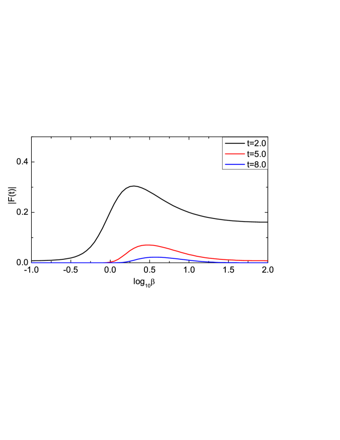
Figure 5: (Color online). The coherence factor $F\left(t\right)$ as a function of temperature $T$ at certain time for Ising ($\gamma$=$1$) spin chain with a size of $N$=$200$. These lines are from the cross-section of Fig 4 at different time $t$.

Now we turn to study the evolution of $F\left(t\right)$ with different initial states in the strong coupling regime. In this regime, $F\left(t\right)$ will oscillate rapidly under a Gaussian envelope Cucc2 ; Cormick2 ; Yuan2 . Following Refs. Cucc2 ; Cormick2 , we derive a formula to approximate the Gaussian envelope. By noting that in the strong coupling regime, $\alpha_{k}^{\left(\lambda_{+-}\right)}\approx\pi/2$, we can simplify Eq. (27) as

$$F\left(t\right)\approx\prod\nolimits_{k=1}^{M}|\exp\left[it\left(\Omega_{k}^{\left(\lambda_{+}\right)}+\Omega_{k}^{\left(\lambda_{-}\right)}\right)\right]\cos^{2}\alpha_{k}^{\left(\lambda_{+i}\right)}+\exp\left[it\left(-\Omega_{k}^{\left(\lambda_{+}\right)}-\Omega_{k}^{\left(\lambda_{-}\right)}\right)\right]\sin^{2}\alpha_{k}^{\left(\lambda_{+i}\right)}|.$$ (40)

The energy terms can be expressed as $\Omega_{k}^{\left(\lambda_{+}\right)}$+$\Omega_{k}^{\left(\lambda_{-}\right)}$=$E$+$\Delta_{k}$. The evolution of $F_{k}\left(t\right)$ oscillates rapidly with almost the same frequency $E\mathtt{\approx}4g$. The differences $\Delta_{k}\mathtt{\ll}E$ are responsible for the decay of the envelope. By evaluation near the peaks of the oscillations, $t$=$n\pi/E$+$\delta t$, and by using the Taylor expansions in $\delta t$ and $\Delta_{k}$, we find that the frequency of the peaks corresponds to the energy

$$E=\frac{\underset{k}{\overset{M}{{\displaystyle\sum}}}\sin^{2}\left(\theta_{k}^{g}-\theta_{k}^{i}\right)\left[\Omega_{k}^{\left(\lambda_{+}\right)}+\Omega_{k}^{\left(\lambda_{-}\right)}\right]}{\underset{k}{\overset{M}{{\displaystyle\sum}}}\sin^{2}\left(\theta_{k}^{g}-\theta_{k}^{i}\right)},$$ (41)

and the value of the envelope at these peaks can be approximated by

$$\tilde{F}\left(t\right)\approx\exp\left\{-\tilde{s}_{M}^{2}t^{2}/2\right\},$$ (42)

where

$$\tilde{s}_{M}^{2}=\sum\left\{\sin^{2}\left(\theta_{k}^{g}-\theta_{k}^{i}\right)\left\{\left[\Omega_{k}^{\left(\lambda_{+}\right)}+\Omega_{k}^{\left(\lambda_{-}\right)}\right]-E\right\}^{2}\right\}.$$ (43)

By noting that for $\gamma$=$1$

$$\underset{k}{{\displaystyle\sum}}\sin^{2}\theta_{k}^{i} \approx\left\{\begin{array}[c]{c}\frac{M}{2\lambda_{i}^{2}}\\ \frac{M}{2}\end{array}\right.\begin{array}[c]{c}\lambda_{i}^{2}>1\\ \lambda_{i}^{2}\leq 1\end{array},$$ (48)

$${\displaystyle\sum}\left(\sin^{2}\theta_{k}^{i}\sin^{2}\frac{2\pi k}{N}\right) \approx\left\{\begin{array}[c]{c}\frac{M}{8}\frac{3\lambda_{i}^{2}-1}{\lambda_{i}^{4}}\\ \frac{M}{8}\left(3-\lambda_{i}^{2}\right)\end{array}\right.\begin{array}[c]{c}\lambda_{i}^{2}>1\\ \lambda_{i}^{2}\leq 1\end{array},$$ (53)

$${\displaystyle\sum}\left(\sin^{2}\theta_{k}^{i}\sin^{4}\frac{2\pi k}{N}\right) \approx\left\{\begin{array}[c]{c}\frac{M}{32\lambda_{i}^{6}}\left(10\lambda_{i}^{4}-5\lambda_{i}^{2}+1\right)\\ \frac{M}{32}\left(10-5\lambda_{i}^{2}+\lambda_{i}^{4}\right)\end{array}\right.\begin{array}[c]{c}\lambda_{i}^{2}>1\\ \lambda_{i}^{2}\leq 1\end{array},$$ (58)

and after a tedious calculation, we obtain the exact expression for $\tilde{s}_{M}^{2}$ as

$$\tilde{s}_{M}^{2}\approx\left\{\begin{array}[c]{c}\frac{M}{8g^{2}\lambda_{i}^{4}}\left(\lambda_{i}^{2}+1\right)\\ \frac{M}{8g^{2}}\left(\lambda_{i}^{2}+1\right)\end{array}\right.\begin{array}[c]{c}\lambda_{i}^{2}>1\\ \lambda_{i}^{2}\leq 1\end{array}.$$ (59)

Similar to the case of weak coupling regime, here we firstly give the expression for the reciprocal of the envelops’s width $\tilde{s}_{M}^{2}$ with the parameters of the Hamiltonian for Ising ($\gamma$=$1$) model. That is, we succeed in using a simple formula to approximate the Gaussian envelope of the evolution of the coherence factor. It is noteworthy that in the strong coupling regime, the formula Eq. (37) is still applicable in very short time ($t\ll 1$). In Fig. 6 we show the numerical results of $F(t)$ as a function of $t$ with $\lambda_{i}$=$0.5$ and $\lambda_{i}$=$1.5$ respectively. The red and blue lines are drawn with Eqs. (27) and (42) respectively with $\lambda_{i}$=$0.5$; The black and yellow lines are drawn with Eqs. (27) and (42) respectively with $\lambda_{i}$=$1.5$. And the value of $\tilde{s}_{M}^{2}$ in Fig. 6 is calculated with Eq. (59). One can see that the approximate envelope fits very well. Also similar to the case of weak coupling regime, the derivative of $\tilde{s}_{M}^{2}$ with $\lambda_{i}^{2}$ is not continuous at the critical point $\lambda_{i}$=$1$.$0$ of the initial Hamiltonian.

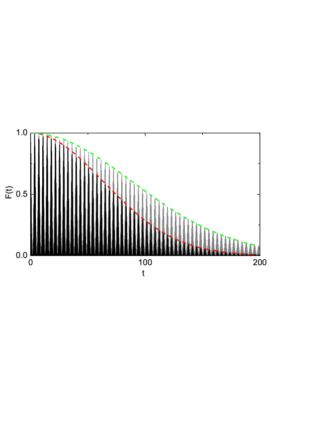
Figure 6: (Color online). The coherence factor $F\left(t\right)$ as a function of time $t$ for Ising ($\gamma$=$1$) spin chain with a size of $N$=$800$ in the strong coupling regime $g$=$500$.

In some previous papers Cucc1 ; Cormick1 , universal regime of the Gaussian envelope has been found when the coupling strength is large enough, which means that the envelope of the decay of the coherence factor in the system is Gaussian with a width independent of the system-environment coupling strength. While obviously, the width of the Gaussian envelope we calculated is proportional to the coupling strength $g$. This seeming conflict originates from the different settings of the Hamiltonian. In Refs. Cucc1 ; Cormick1 , only one of $\lambda_{-}$ and $\lambda_{+}$ is correlated with the coupling strength $g$, the other is uncorrelated with $g$. This setting leads to different results of $F(t)$ and thus the width of the envelope.

In conclusion, we have studied the decaying process of the coherence factor of a coupled system consisting of a central spin and its correlated environment described by a general $XY$ spin-chain model. We mainly analyzed the dependence of the decoherence on the initial state of the environmental Hamiltonian by assuming that the initial state is the ground state of the initial Hamiltonian $H_{E}^{\left(\lambda_{i}\right)}$ at time $t$=$0$ which may be different from the evolving Hamiltonian $H_{E}^{\left(\lambda_{e}\right)}$. In this case we have obtained the exact analytical expression for the decoherence factor $F\left(t\right)$. At the critical point $\lambda_{e}$=$1$ of the evolving Hamiltonian, the coherence factor $F\left(t\right)$ decays rapidly from unity to zero for any value of $\lambda_{i}$ and with no revivals when the site number $N$ is large enough. The evolution of the coherence factor $F\left(t\right)$ as a function of time $t$ is Gaussian in a short time whenever in weak or strong coupling regime. In the strong coupling regime, $F\left(t\right)$ oscillates rapidly under a Gaussian envelope. In this case, as a main result, we have obtained a simple expression for the Gaussian decay and the Gaussian envelope with the parameters of the Hamiltonian for Ising ($\gamma$=$1$) model. All these approximate expressions fit the evolution of the coherence factor or the envelope very well. We have also chosen thermal equilibrium state as initial state and found that the decaying speed of $F\left(t\right)$ dose not increase monotonously with temperature for certain time $t$.

This work was supported by NSFC under Grants No. 11147143, No. 11204012, and No. 91321103.

References

(1)W. H. Zurek. Rev. Mod. Phys. 75, 715–775, (2003).