Hamiltonians of Spherical Galaxies in Action-Angle Coordinates

Abstract

We present a simple formula for the Hamiltonian in terms of the actions for spherically symmetric, scale-free potentials. The Hamiltonian is a power-law or logarithmic function of a linear combination of the actions. Our expression reduces to the well-known results for the familiar cases of the harmonic oscillator and the Kepler potential. For other power-laws, as well as for the singular isothermal sphere, it is exact for the radial and circular orbits, and very accurate for general orbits. Numerical tests show that the errors are always very small, with mean errors across a grid of actions always $<1$ percent and maximum errors $<2.5$ percent. Simple first-order corrections can reduce mean errors to $<0.6$ percent and maximum errors to $<1$ percent.

We use our new result to show that: [1] the misalignment angle between debris in a stream and a progenitor is always very nearly zero in spherical scale-free potentials, demonstrating that streams can sometimes be well-approximated by orbits, [2] the effects of an adiabatic change in the stellar density profile in the inner region of a galaxy weaken any existing $1/r$ dark matter density cusp, which is reduced to $1/r^{1/3}$. More generally, we derive the full range of adiabatic cusp transformations and show that a $1/r^{\gamma_{0}}$ density cusp may be changed to $1/r^{\gamma_{1}}$ only if $\gamma_{0}/(4-\gamma_{0})\leq\gamma_{1}\leq(9-2\gamma_{0})/(4-\gamma_{0})$. It follows that adiabatic transformations can never completely erase a dark matter cusp.

1 INTRODUCTION

Action-angle coordinates are an extremely useful set of coordinates with which to describe a stellar system. Actions are integrals of motion given by

$$J_{i}=\dfrac{1}{2\pi}\oint_{\gamma_{i}}\boldsymbol{p}.\mathrm{d}\boldsymbol{q},$$ (1)

where $\gamma_{i}$ is a closed path around an orbital torus, and $(\boldsymbol{p},\boldsymbol{q})$ are canonically conjugate phase-space coordinates. Since actions are integrals of motion, they satisfy $\dot{J_{i}}=0$, greatly simplifying Hamilton’s equations for the canonically conjugate angle variables. These follow the trivial time evolution

$$\theta_{i}(t)=\theta_{i}(0)+\Omega_{i}t,\qquad\qquad\Omega_{i}=\frac{\partial H}{\partial J_{i}}.$$ (2)

Already, we can see the appeal of the action-angle coordinate space. In the physical phase-space $(\boldsymbol{x},\boldsymbol{v})$, each of the six phase-space coordinates generally evolves in a complicated fashion. In $(\boldsymbol{J},\boldsymbol{\theta})$ space, three of the coordinates are constant and the other three evolve linearly with time. Action-angle space is the natural arena in which to view stellar orbits.

The benefit of action-angles extends beyond their simple time evolution, however. Despite the fact that galaxies are never truly in a steady state, equilibrium models are hugely important tools in developing our understanding of galaxies. Using equilibrium models, we can infer the gravitational potential of a galaxy and predict all observable quantities. Under most circumstances, we are justified in assuming that a galaxy is always close to an equilibrium state, and we can model non-equilibrium effects such as accretion or stellar evolution as small perturbations to the system.

Given the assumption of dynamical equilibrium, the most efficient way to proceed is via the use of the Jeans theorem (see Binney & Tremaine 2008), which tells us that the phase-space distribution function (hereafter DF) of a galaxy or stellar system in equilibrium may be written as a function of just three isolating integrals. This reduces the dimensionality of the space under consideration from six to three, and so invoking the Jeans theorem leads to an elegant simplification of the modelling problem. Since actions are adiabatic invariants, if we choose to write the DF as a function of the actions, its functional form is preserved under slow changes to the galaxy. This property can be exploited to model various processes in galaxy evolution. For example, Goodman & Binney (1984) showed that the adiabatic growth of mass at the centre of a stellar system causes the velocity dispersion to become tangentially distended, a process invoked by Agnello et al. (2014) to explain the kinematics of M87’s globular cluster populations. Similarly, Katz et al. (2014) recently modelled the adiabatic compression of dark matter halos in galaxies from the THINGS survey to reproduce their rotation curves. Another example is provided by Gondolo & Silk (1999), who showed that the adiabatic growth of a black hole can cause a dark matter spike at the center of a cusped dark halo.

Unfortunately, although action-angles are very useful when known, they are not usually available analytically. In fact, Evans et al. (1990) showed that the most general potential in which the actions are available as elementary functions is the isochrone (which reduces to the Kepler and harmonic potentials in limiting cases). Recent efforts by Binney (2012), Bovy (2014) and Sanders & Binney (2014) mean that actions can now be numerically recovered in many potentials, but analytical approximations are still sparse. Though numerical methods are ultimately the most widely applicable, analytical approximations are important insofar as they give us valuable insight into the properties of a system, not to mention drastically reduced computational time when they are sufficiently accurate.

In this paper, we present a new method for finding accurate approximations to the Hamiltonians of spherically symmetric, scale-free systems and apply it to general power-law potentials and the isothermal sphere. We then use the method in two applications: finding the misalignment angle of a stellar stream, and calculating the effect of a slowly changing central stellar density profile on the slope of a dark matter cusp.

2 Method

In a spherical potential, the radial action is given by

$$J_{r}=\dfrac{1}{2\pi}\oint\sqrt{2E-2\Phi(r)-L^{2}/r^{2}}\mathrm{d}r.$$ (3)

The angular actions are related to the angular momentum components via $J_{\phi}=|L_{z}|$ and $J_{\theta}=L-|L_{z}|$, where $L=J_{\theta}+J_{\phi}$ is the total angular momentum and $L_{z}$ is the angular momentum about the $z$-axis. The Hamiltonian can then be regarded as a function of just two quantities: $H\equiv H(L,J_{r})$. The most general method of finding $H(L,J_{r})$ is to solve the integral equation (3) for $E$ but, as previously mentioned, this cannot be done for the general case.

We now present a prescription for finding approximations $\mathcal{H}(L,J_{r})$ to the exact Hamiltonian $H(L,J_{r})$ of a spherical, scale-free potential $\Phi(r)$. In terms of the usual phase-space coordinates, the Hamiltonian is given by

$$H(r,\boldsymbol{v})=\frac{1}{2}\boldsymbol{v}^{2}+\Phi(r).$$ (4)

We now look to find an approximate transformation by considering only the two most basic types of orbit: radial and circular orbits. For the radial orbits, we must evaluate

$$J_{r}=\dfrac{1}{2\pi}\oint\sqrt{2E(0,J_{r})-2\Phi(r)}\mathrm{d}r$$ (5)

and invert the resulting expression for $E(0,J_{r})$. The energy of the circular orbits is given by the system of simultaneous equations

$$L(r)=rv_{\rm c}(r),\qquad\qquad E(L,0)=\frac{1}{2}v_{\rm c}(r)^{2}+\Phi(r),$$ (6)

where $v_{\rm c}(r)$ is the circular speed. For a scale-free potential, simply as a consequence of dimensional analysis, both results will have the same functional form

$$E(J_{i},J_{j}=0)=f(a_{i}J_{i}),$$ (7)

where $f(x)$ is some function and $a_{i}$ is a constant. This means that a natural choice of interpolation for a general orbit is

$$\mathcal{H}(L,J_{r})=f(aL+bJ_{r}),$$ (8)

where $a$ and $b$ are found using the solutions to Eqs. (5) and (6). Therefore, as long as $a$ and $b$ are available, one has a very simple analytical approximation to the true Hamiltonian of any scale-free spherical system.

If our Hamiltonian is not scale-free, we can often break the problem up into scale-free regimes, and devise an interpolation formula that smoothly matches the limits. A specific example of this is provided by Evans & Williams (2014), who provided a Hamiltonian $\mathcal{H}(L,J_{r})$ for a halo model with a $1/r$ density cusp at the center but a flat rotation curve at large radii.

3 Power-Law Potentials

3.1 Results

Let us now consider power-law potentials of the form

$$\Phi(r)=Ar^{\alpha},\qquad A={v_{0}^{2}\over\alpha r_{0}^{\alpha}}.$$ (9)

The choice of constant $A$ is motivated by the rotation law, which takes the form

$$v_{\rm c}^{2}(r)=v_{0}^{2}\left({r\over r_{0}}\right)^{\alpha}.$$ (10)

So, the rotation curve has the value $v_{0}$ at reference radius $r_{0}$. Models with $\alpha>0$ (or $\alpha<0$) have a rising (or falling) rotation curve. The model with $\alpha=0$ has a flat rotation curve, and is recognised as the singular isothermal sphere. To recover its familiar logarithmic potential, we must add a constant $-v_{0}^{2}/\alpha$ to eq. (9) and use L’Hôpital’s rule to take carefully the limit $\alpha\rightarrow 0$. The physical range of $\alpha$ is $-1\leq\alpha\leq 2$, with the extremes representing a Keplerian potential (point mass) and a harmonic potential (homogenous matter distribution) respectively.

Applying our method to case when $A,\alpha>0$ (the rising rotation curve case), we find

$$E(0,J_{r}) = \bigg{[}\dfrac{\sqrt{2\pi}\alpha A^{1/\alpha}\Gamma(3/2+1/\alpha)}{\Gamma(1/\alpha)}\bigg{]}^{\beta}J_{r}^{\beta},$$

$$E(L,0) = \dfrac{(A\alpha)^{\beta/\alpha}}{\beta}L^{\beta},$$ (11)

where we have set $\beta=2\alpha/(\alpha+2)$. This implies that $f(x)\propto x^{\beta}$. This gives us the following very simple approximation for the Hamiltonian

$$\mathcal{H}(L,J_{r})=C(L+DJ_{r})^{\beta},$$ (12)

where the constants $C$ and $D$ are

$$C = \dfrac{v_{0}^{2\beta/\alpha}}{r_{0}^{\beta}\beta},$$ (13)

$$D = \dfrac{\sqrt{2\pi}\Gamma(3/2+1/\alpha)\alpha^{-1/\alpha}\beta^{1/\beta}}{\Gamma(1+1/\alpha)}.$$

This prescription may be tested on the special case of the harmonic oscillator ($\alpha=2$). Setting $A=\frac{1}{2}\Omega^{2}$, we recover the well-known exact analytical result (see, for example, Goldstein 1980)

$$\mathcal{H}(L,J_{r})=2\Omega J_{r}+\Omega L.$$ (14)

So, $\mathcal{H}$ perfectly coincides with the true Hamiltonian $H$ for the harmonic oscillator.

When $A,\alpha<0$ (the falling rotation curve case), the result is the same as eq. (12), except

$$D=\dfrac{\sqrt{2\pi}\Gamma(1-1/\alpha)(-\alpha)^{1-1/\alpha}(-\beta)^{1/\beta}}{\Gamma(-1/\alpha-1/2)}.$$ (15)

The obvious test in this case is the Keplerian potential, where $A=-GM$ and $\alpha=-1$, which gives:

$$\mathcal{H}(L,J_{r})=-\dfrac{1}{2}\bigg{(}\dfrac{GM}{L+J_{r}}\bigg{)}^{2}.$$ (16)

This coincides with the exact result for the Kepler potential, derived by the residue calculus in Born (1927) and repeated in Goldstein (1980).

The case of the flat rotation curve (or the singular isothermal sphere) can be derived by taking the limit $\alpha\rightarrow 0$ and using L’Hôpital’s rule. The potential becomes logarithmic $\Phi=v_{0}^{2}\log r/r_{0}$, and so we find that $f(x)\propto\log(x)$. Our approximation then gives

$$\mathcal{H}(L,J_{r})=v_{0}^{2}\log\bigg{(}\dfrac{\sqrt{e}L+\sqrt{2\pi}J_{r}}{v_{0}r_{0}}\bigg{)},$$ (17)

as stated in Evans & Williams (2014).

So, we have found a surprisingly simple and compact formula (12) for the Hamiltonian in terms of the actions valid for any power-law potential with $-1\leq\alpha\leq 2$. It is exact for the two classical cases – the Kepler potential and the harmonic oscillator – which have been known for over a century. Notice too that the frequencies $\Omega_{i}$ are rationally related only in the case of the Kepler potential and the harmonic oscillator. Thus, we have recovered Bertrand’s theorem (see e.g., Goldstein, 1980), which states that the only central force laws with everywhere closed bound orbits are the linear and inverse square force laws. For all other cases, our formula (12) gives frequencies that are incommensurable and so the motion is conditionally periodic.

3.2 Errors and First Order Corrections

Given that the approximation is only exact for the cases $\alpha=-1$ and $\alpha=2$, we tested the effectiveness of the approximation for several values of $\alpha$: $-0.5$, $0$ (the isothermal sphere), $0.5$, $1$, and $1.5$. In each case we evaluate a set of 10000 orbits on a grid of pericenter and apocenter radii: $r_{p}=0\rightarrow 50$, $r_{a}=0\rightarrow 100$. For each orbit we evaluate the energy and angular momentum, which are available as algebraic expressions in terms of pericenter and apocenter radii (Lynden-Bell, 2010), and the radial action, which requires the evaluation of a numerical integral. This results in an irregularly spaced grid in action space.

Before discussing numerical values, it is necessary to explain how we define errors across the sequence of models. We consider correction terms of the form

$$\mathcal{H}=f(aL+bJ_{r}+\epsilon\sqrt{LJ_{r}}).$$ (18)

where $f(x)\propto x^{\beta}$ (if $\beta\neq 0$) or $f(x)\propto\log x$ (if $\beta=0$). Due to lack of dimensional constants in the problem, the correction must possess the dimensions of actions. Its form is suggested by examing the error distribution along rays in action space. A measure of the fractional error between the corrected values and the original approximation is then

$$\dfrac{\Delta\mathcal{H}^{1/\beta}}{\mathcal{H}^{1/\beta}}=\dfrac{\epsilon\sqrt{LJ_{r}}}{aL+bJ_{r}+\epsilon\sqrt{LJ_{r}}}\approx\dfrac{\epsilon\sqrt{LJ_{r}}}{aL+bJ_{r}},$$ (19)

In the isothermal case ($\beta=0$), this becomes

$$\dfrac{\Delta\mathcal{\exp H_{\mathrm{iso}}}}{\exp\mathcal{H}_{\mathrm{iso}}}\approx\dfrac{\epsilon\sqrt{LJ_{r}}}{aL+bJ_{r}}.$$ (20)

and so the measure of error is a continuous function of power-law index $\alpha$.

We find that the errors in all cases are very small. The mean absolute percentage error on the action grid is $<1$ percent in every case, and the maximum absolute percentage error is always $<2.5$ percent. These results are given in Fig. 1. The distribution of errors is very similar in all cases: it is scale-free and maximised along a particular ray in action space. A typical example is given in Fig. 2.

Given the simplicity of the error distribution, we can calculate a value for $\epsilon$ in Eq. (18) very easily. Assuming the errors are maximised along the line $L=\chi^{2}J_{r}$, we can substitute this into Eqs. (19) or (20) to give

$$\epsilon=\dfrac{\delta_{\mathrm{max}}(\chi^{2}a+b)}{\chi}$$ (21)

where $\delta_{\mathrm{max}}$ is the fractional error with the largest absolute value on the grid. We carried out this analysis for each of our test cases and found that it had a significant effect on the maximum error on the grid, as well as reducing the average error in every case. These results are also given in Fig. 1. If these first-order corrections are included, the error never exceeds $1$ percent for any of our test cases.

On account of its astrophysical importance, we give the expression for the first-order corrected formula for the singular isothermal sphere:

$$\mathcal{H} = v_{0}^{2}\log\bigg{(}\dfrac{\sqrt{e}L+\sqrt{2\pi}J_{r}+\epsilon\sqrt{LJ_{r}}}{v_{0}r_{0}}\bigg{)},$$ (22)

$$\epsilon = -0.1009.$$

For the case $\alpha=1$, which corresponds to the cosmologically motivated $1/r$ or Navarro-Frenk-White (1996) density cusp, the corrected expression is

$$\mathcal{H} = {3v_{0}^{4/3}\over 2r_{0}^{2/3}}\bigg{(}L+{\pi\over\sqrt{3}}J_{r}+\epsilon\sqrt{LJ_{r}}\bigg{)}^{2/3},$$ (23)

$$\epsilon = -0.0412.$$

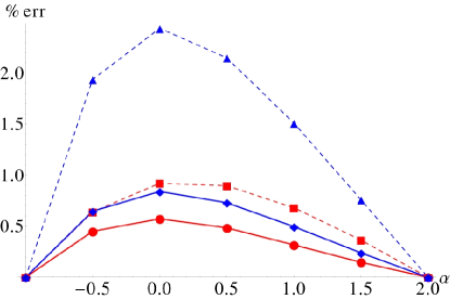
Figure 1: Absolute percentage errors against power-law index ($\alpha=0$ corresponds to the isothermal sphere). The dashed lines correspond to the original approximation, and the solid lines include first-order corrections. Blue lines are maximum absolute percentage errors across the action grid, red lines are the mean absolute percentage errors. One can see that the first-order corrections reduce the maximum error significantly, and also have a noticeable effect on the mean error.

4 Applications

Here, we present two simple applications of our results. The first is to stellar streams. We demonstrate that within this approximation streams are well delineated by orbits. The second is to cusps in the centre of galaxies. We show that the central slope of a dark matter halo is reduced when the stellar populations begin to dominate the potential.

4.1 Stellar Streams

Sanders & Binney (2013) showed that a stream can only be successfully modelled by an orbit if the misalignment angle is very small. This angle is given by

$$\varphi=\arccos(\hat{\boldsymbol{\Omega}}.\hat{\boldsymbol{e}}_{1}),$$ (24)

where $\hat{\boldsymbol{\Omega}}$ is the normalised frequency vector of the progenitor of the stellar stream and $\hat{\boldsymbol{e}}_{1}$ is the leading eigenvector of the Hessian matrix

$$D_{ij}(\hat{J})=\frac{\partial^{2}H}{\partial J_{i}\partial J_{j}}.$$ (25)

The misalignment angle quantifies the offset in angle space between stripped material and the progenitor, and encodes the direction in which stars spread in action-angle space. For a long, thin stream to form, the Hessian must have one dominant eigenvalue. We now evaluate $D_{ij}$ within our approximate framework. Any approximate Hamiltonian produced by our method is of the form

$$\mathcal{H}(L,J_{r})=f(aL+bJ_{r}),$$ (26)

giving rise to a Hessian matrix

$$D_{ij}(\hat{J})=G(L,J_{r})\left(\begin{array}[]{cc}a^{2}&ab\\ ab&b^{2}\end{array}\right).$$ (27)

Such a matrix has only one non-zero eigenvalue, $\lambda=G(a^{2}+b^{2})$, with corresponding eigenvector

$$\hat{\boldsymbol{e}}_{1}=\dfrac{1}{\sqrt{a^{2}/b^{2}+1}}\left(\begin{array}[]{c}a/b\\ 1\end{array}\right).\$$ (28)

Now, if we evaluate a general frequency vector using $\mathcal{H}$, we find

$$\hat{\boldsymbol{\Omega}}\propto\hat{\boldsymbol{e}}_{1}.$$ (29)

This implies that the misalignment angle vanishes, and so the stream will always develop along an orbit under this approximation. This suggests that, at least in the scale-free spherical case, the misalignment angle must be very small and therefore the stream should be very well approximated by an orbit. This may provide a measure of justification for the assumption used in Koposov et al. (2010), in which the GD1 stream (Grillmair & Dionatos, 2006) was assumed to lie along an orbit in a scale-free, mildly axisymmetric potential.

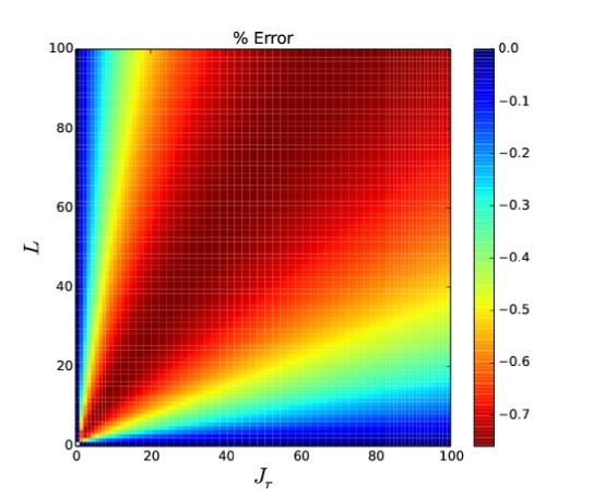
Figure 2: Distribution of percentage error with actions for the case $\alpha=1.5$. One can see a definite systematic trend that could be removed with an astute choice of first order correction.

4.2 Adiabatic Transformation of Density Cusps

Navarro, Frenk & White (1996) famously discovered that, in dissipationless simulations, dark haloes form a $1/r$ density cusp in the centre of galaxies. However, there is a discrepancy between the predicted density of dark matter at the center of spiral galaxies and the inferred dark matter density consistent with observations. For example, in the case of the Milky Way, Binney & Evans (2001) show that cuspy dark matter density haloes would violate constraints on the rotation curve, given the known contributions from the stellar and ISM disks and Galactic bar. Clearly, the $1/r$ cusp, if it originally formed in the Milky Way galaxy, has been weakened with the passage of time.

We assume that the dark halo of the galaxy formed first, and that the dark matter density in the center of a galaxy originally followed a $1/r$ cusp. With the build-up of the disk and bulge stellar populations, we assume that the the density profile of the dominant stellar populations becomes roughly constant in the very central parts. In this instance, the potential is initially linear ($\alpha_{0}=1$), corresponding to the Navarro-Frenk-White cusp, and becomes harmonic, ($\alpha_{1}=2$), corresponding to a constant density core. Assuming that this process occurs sufficiently slowly that the adiabatic invariance of the actions holds good, then we can find the final profile of the dark matter.

For the collisionless dark matter, we use the self-consistent power-law DF derived by Evans (1994) (Eq. 5.4), and assume an initially isotropic population so that

$$f(E)=\mathcal{N}E^{-\dfrac{\alpha_{0}+4}{2\alpha_{0}}},$$ (30)

where $\mathcal{N}$ is a normalisation factor. We then insert our approximation for $H(L,J_{r})$ from Eq. (13) for the case $\alpha=\alpha_{0}=1$ to find

$$f(L,J_{r})\simeq\mathcal{M}\bigg{(}L+\dfrac{\pi J_{r}}{\sqrt{3}}\bigg{)}^{-5/3},$$ (31)

where $\mathcal{M}$ is a new normalisation factor. Since the changes in the potential are presumed to occur adiabatically, the distribution function is always of this form, even at the endpoint. We now eliminate $J_{r}$ by again using Eq. (13) but for the final potential, $\Phi_{1}=\frac{1}{2}\Omega^{2}r^{2}$ (which is exact in this case), giving:

$$f(L,J_{r})\propto\bigg{(}L+\dfrac{\pi}{2\sqrt{3}}\bigg{[}\dfrac{H}{\Omega}-L\big{)}\bigg{]}\bigg{)}^{-5/3}$$ (32)

and substitute for $H$ using Eq. (4), which finally leaves

$$f(L,J_{r})\propto\bigg{(}\big{(}1-\dfrac{\pi}{2\sqrt{3}}\big{)}L+\dfrac{\pi}{2\Omega\sqrt{3}}\big{(}\frac{1}{2}\boldsymbol{v}^{2}+\frac{1}{2}\Omega^{2}r^{2}\big{)}\bigg{)}^{-5/3}.$$ (33)

We can simplify this rather messy looking expression. The first term is proportional to $L$, which will be small for particles that penetrate the centre of the galaxy. This term also has a considerably smaller numerical prefactor than the isotropic term. On this basis, we consider only the second term and integrate over velocity space to find the spatial dependence of the final density profile

$$\rho_{\mathrm{dm}}(r)\propto\int_{0}^{\infty}\dfrac{v^{2}\mathrm{d}v}{\bigg{(}v^{2}+\Omega^{2}r^{2}\bigg{)}^{5/3}}.$$ (34)

This integral can be evaluated using the substitution $v^{2}=\Omega^{2}r^{2}\tan^{2}\theta$, and gives the final result

$$\rho_{\mathrm{dm}}(r)\propto r^{-1/3}.$$ (35)

So, we have found that the density profile of dark matter particles that initially followed a $r^{-1}$ density cusp has developed a shallower density profile of $r^{-1/3}$ as the density becomes homogeneous in the very central parts.

This calculation can be carried out completely generally. Suppose the initial dark matter cusp has form $r^{-\gamma_{0}}$. Let the gravitational potential evolve so that the final end-state has $\phi\propto r^{\alpha_{1}}$. Then the final dark matter density cusp behaves like $r^{-\gamma_{1}}$, where

$$\gamma_{1}(\gamma_{0},\alpha_{1})={\gamma_{0}-\alpha_{1}(\gamma_{0}-3)-6\over\gamma_{0}-4}.$$ (36)

Our earlier result (35) corresponds to the special case of an NFW cusp responding to a potential that slowly changes to harmonic, that is $\gamma_{1}(1,2)=1/3$

This equation enables us to map out the domain of accessible adiabatic changes of cusp slope, as shown in Fig. 3. The upper line corresponds to $\gamma_{1}(\gamma_{0},-1)$, in which the underlying potential is slowly changed to Keplerian and the matter distribution becomes strongly concentrated. The lower line corresponds to $\gamma_{1}(\gamma_{0},2)$, as the potential is changed to harmonic and the matter distribution becomes homoegeneous. The starting cusp $\gamma_{0}$ may be adiabatically transformed into $\gamma_{1}$ provided

$${\gamma_{0}\over 4-\gamma_{0}}\leq\gamma_{1}\leq{9-2\gamma_{0}\over 4-\gamma_{0}}$$ (37)

This region is shown unshaded in Fig. 3. It is the domain of accessible cusp transformations. Notice that an initial NFW cusp can only ever be adiabatically transformed into a cusp with slope $1/3\leq\gamma_{1}\leq 7/3$. It can never be completely erased. Of course, this result is restricted to adiabatic changes. There are a variety of non-adiabatic processes that are widely believed to remove cusps, including repeated mass loss (Read & Gilmore, 2005), AGN driven outflows (Martizzi et al., 2013) and infall of satellites (El-Zant et al., 2001).

Finally, we note that Gondolo & Silk (1999), in their study of the response of a dark matter cusp to a growing black hole, derived the limit $\gamma_{1}(\gamma_{0},-1)$, though only for models with $0<\gamma_{0}<2$. The formula is generally valid throughout the entire physical range $0\leq\gamma_{0}\leq 3$, though the methods employed by Gondolo & Silk (1999) were unable to include isothermal cusp slopes and steeper.

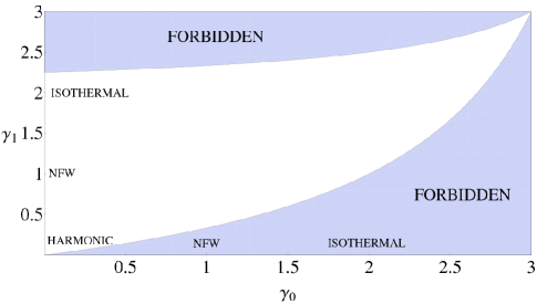
Figure 3: The domain of allowed cusp slope transformations. The final cusp slope $\gamma_{1}$ is plotted against the initial cusp slope $\gamma_{0}$. Shaded regions cannot be reached by adiabatic changes. The upper line corresponds to $\gamma_{1}(\gamma_{0},-1)$ (the Keplerian limit) and the lower line to $\gamma_{1}(\gamma_{0},2)$ (the harmonic limit).

5 Conclusions

Action-angle coordinates are a powerful tool in modern classical mechanics  (see e.g., Abraham & Marsden, 1978; Arnold, 1989) and galactic dynamics (Binney & Tremaine, 2008). Their widespread use is hampered by the fact that the actions can be difficult to find explicitly. Although numerical tools are becoming available to make this job easier (Binney, 2012; Bovy, 2014; Sanders & Binney, 2014), there are disappointingly few potentials for which analytic results are possible.

The main result of the paper is the discovery of a simple formula for the Hamiltonian of scale-free potentials in terms of the actions. The formula recovers the well-known and exact results for the harmonic oscillator and Keplerian potentials, which have been known for over a century (see e.g., Goldstein, 1980). For other power-laws, the formula is exact for radial and circular orbits, but approximate for general orbits. However, numerical tests show that the the errors are always very small, with mean errors across a grid of actions always $<1$ percent, and maximum errors never larger than $2.5$ percent. Our formula therefore provides a useful and accurate approximate Hamiltonian for many of the commonly used galactic potentials, including the isothermal sphere and power-law cusps. It may also be improved with simple first-order corrections if need be, which reduce the mean error to always $<0.6$ percent, and the maximum error $<1$ percent.

We provided two applications. First, the mismatch of streams from their progenitor is described by a misalignment angle. This in turn is controlled by the Hessian of the Hamiltonian with respect to the actions (Sanders & Binney, 2013). Most streams in the Milky Way halo occur at Galactocentric radii greater than 20 kpc, so that the potential is probably scale-free to a good approximation. If, in addition, the potential is nearly spherical, then the misalignment angle may be close to zero. This suggests that there may be regimes in which the approximation of thin streams by orbits is a reasonable one.

Second, we considered the evolution of a dark matter $1/r$ density cusp in a spiral galaxy. Although $1/r$ density cusps are known to be the endpoint of dissipationless simulations, there is ample evidence that in galaxies like the Milky Way, any such cusp must have been modified at the center (Binney & Evans, 2001). The response of a $1/r$ cusp to the slow build-up of a stellar bulge and disk can be computed using our formula, under the assumption of adiabatic invariance. As the overall potential becomes cored and harmonic, the dark matter density cusp becomes shallower and is nearly erased. It began as a $1/r$ and finished as $1/r^{1/3}$ density cusp. Considering the more general problem of density cusps of arbitrary slope, we show that adiabatic transformations can only weaken, and never remove, such cusps. A density singularity – once present – requires some non-adiabatic process to erase it.

In this paper, we only considered scale-free potentials. Nonetheless, our methods can also be applied to spherical potentials that possess a scale-length. This requires more work because we have to devise a suitable interpolation scheme to sew the different regimes together, but it is still very effective. Evans & Williams (2014) provide a specific example, but it would be interesting to study this problem in greater generality.

Also looking to the future, it is worthwhile to consider whether similar reasoning could be applied to scale-free, axisymmetric potentials. The regularity of Poincaré surfaces of sections for axisymmetric scale-free potentials  (Richstone, 1982; Evans, 1994) strongly hints that there are simple results to be found. This is a more complex problem, given that there are now three actions to consider rather than the two in the spherical case ($J_{r}$ and $J_{\theta}+J_{\phi}$). Nonetheless, we can consider three special orbits: purely vertical orbits, purely radial orbits and circular orbits in the plane, for which the actions are well-defined. For example, the flattened logarithmic potential is

$$\Phi(R,z)=\dfrac{1}{2}v_{0}^{2}\log\bigg{(}(R/r_{0})^{2}+(z/qr_{0})^{2}\bigg{)}.$$ (38)

Using the same interpolation techniques, we reach the following expression for an approximate Hamiltonian:

$$\mathcal{H}=v_{0}^{2}\log\bigg{(}\dfrac{\sqrt{2\pi}(J_{R}+J_{z}/q)+\sqrt{e}|L_{z}|}{v_{0}r_{0}}\bigg{)}.$$ (39)

Given the fact that the actions cannot be written down as a quadratures for general orbits in this potential, this expression would have to be tested using an approximate method, such as described in Binney (2012). We look to do exactly this in future investigations.

References

- Abraham & Marsden (1978) Abraham R., Marsden J., 1978, Foundations of Mechanics. Benjamin Cumings
- Agnello et al. (2014) Agnello A., Evans N. W., Romanowsky A. J., Brodie J.-P., 2014, ArXiv e-prints
- Arnold (1989) Arnold V., 1989, Mathematical Methods of Classical Mechanics. Springer Verlag
- Binney (2012) Binney J., 2012, MNRAS, 426, 1324
- Binney & Tremaine (2008) Binney J., Tremaine S., 2008, Galactic Dynamics: Second Edition. Princeton University Press
- Binney & Evans (2001) Binney J. J., Evans N. W., 2001, MNRAS, 327, L27
- Born (1927) Born M., 1927, The Mechanics of the Atom. G. Bell and Sons
- Bovy (2014) Bovy J., 2014, ArXiv e-prints
- El-Zant et al. (2001) El-Zant A., Shlosman I., Hoffman Y., 2001, ApJ, 560, 636
- Evans (1994) Evans N. W., 1994, MNRAS, 267, 333
- Evans et al. (1990) Evans N. W., de Zeeuw P. T., Lynden-Bell D., 1990, MNRAS, 244, 111
- Evans & Williams (2014) Evans N. W., Williams A. A., 2014, ArXiv e-prints
- Goldstein (1980) Goldstein H., 1980, Classical Mechanics: Second Edition. Addison-Wesley
- Gondolo & Silk (1999) Gondolo P., Silk J., 1999, Physical Review Letters, 83, 1719
- Goodman & Binney (1984) Goodman J., Binney J., 1984, MNRAS, 207, 511
- Grillmair & Dionatos (2006) Grillmair C. J., Dionatos O., 2006, ApJL, 643, L17
- Katz et al. (2014) Katz H., McGaugh S. S., Sellwood J. A., de Blok W. J. G., 2014, MNRAS, 439, 1897
- Koposov et al. (2010) Koposov S. E., Rix H.-W., Hogg D. W., 2010, ApJ, 712, 260
- Lynden-Bell (2010) Lynden-Bell D., 2010, MNRAS, 402, 1937
- Martizzi et al. (2013) Martizzi D., Teyssier R., Moore B., 2013, MNRAS, 432, 1947
- Navarro et al. (1996) Navarro J. F., Frenk C. S., White S. D. M., 1996, ApJ, 462, 563
- Read & Gilmore (2005) Read J. I., Gilmore G., 2005, MNRAS, 356, 107
- Richstone (1982) Richstone D. O., 1982, ApJ, 252, 496
- Sanders & Binney (2013) Sanders J. L., Binney J., 2013, MNRAS, 433, 1813
- Sanders & Binney (2014) Sanders J. L., Binney J., 2014, ArXiv e-prints