Abstract

We consider a model of neutrino mass based on R-parity violating (RPV) supersymmetry, with three $\mu_{i}$, relevant for bilinear RPV terms, and three $\lambda^{\prime}_{ijk}$, relevant for the trilinear terms. The present neutrino data, after a precise determination of the mixing angle $\theta_{13}$, severely constrain such models. We make a thorough study of one such class of models that may have interesting signatures at the upgraded LHC. In this class of models, the relevant trilinear couplings are of the form $\lambda^{\prime}_{i33}$, so if the lighter stop squark $\tilde{t}_{1}$ is the lightest supersymmetric particle (LSP), it will decay only through these couplings, giving rise to events with isolated hard leptons and jets. Even when $\tilde{t}_{1}$ is the next-to-LSP (NLSP), it can decay via the tiny $\lambda^{\prime}$ couplings allowed by the neutrino data, although it may face stiff competition from some R-parity conserving decay modes. Using a simple Pythia based simulation, we find that in both the cases the signal consisting of a pair of oppositely charged leptons ($ee$, $\mu\mu$ or $e\mu$) plus jets may be observable at the upgraded LHC experiments for a reasonable range of the $\tilde{t}_{1}$ mass.

PACS no.: 12.60.Jv, 14.60.Pq, 14.80.Ly

1 Introduction

While the Standard Model (SM) has been vindicated [1], no less by the recent discovery of the Higgs boson [2, 3], as the correct theory of elementary particles at the electroweak scale, there are reasons to suspect that it is at most an effective theory, to be superseded by a more complete theory at a higher energy scale. One of the reasons is the tiny but nonzero neutrino mass, unaccounted for in the SM, whose existence has been inferred from the solar, atmospheric, and reactor neutrino experiments confirming the idea of neutrino oscillation [4]. The smallness of neutrino mass, and the apparent absence of right-handed neutrinos, associated with the fact that neutrinos, being charge-neutral, can very well be their own antiparticles, hints at the possibility that the neutrino mass terms might be purely Majorana in nature. This in turn necessitates the presence of lepton number violating interactions, which are absent in the SM.

Another reason to believe in the incompleteness of the SM is the fine-tuning problem of the Higgs boson mass [5]. Unlike the fermion and gauge boson mass terms, a scalar mass term does not spoil any symmetry of the action, so there is no reason why the quantum corrections to the mass would not drive it to the scale up to which the SM is valid. If the SM is valid all the way up to the Planck scale $M_{Pl}=1/\sqrt{G_{N}}\sim{\cal O}(10^{19})$ GeV, this brings in a very unnatural fine-tuning in the theory, and this is considered a sufficient motivation for physics beyond the SM (BSM). While there are several options to avoid the fine-tuning problem, none of them are experimentally verified; however, supersymmetry (SUSY) [6] remains the most preferred option.

Baryon number $B$ and lepton number $L$ are accidental symmetries of the SM and there is a priori no reason why the SUSY action would respect such symmetries. However, if both of them are violated, protons would decay uncomfortably fast. To prevent that, one imposes an ad hoc $Z_{2}$ symmetry on the action, which is called the R-parity [6], defined as $R_{p}=(-1)^{3B+L+2S}$ where $S$ is the spin of the particle, making $R_{p}=+1(-1)$ for all particles (superparticles or sparticles). This forbids both $B$ and $L$ violating interactions as well, and makes the lightest SUSY particle (LSP) stable, which can be a good cold dark matter (CDM) candidate [7]. This model is commonly known as the R-parity conserving (RPC) SUSY. The lightest neutralino (${\tilde{\chi}}_{1}^{0}$), a weakly interacting massive particle (WIMP), is one of the most suitable CDM candidates.

On the other hand, one might allow either $B$ or $L$ (but not both) violating interactions, which will still forbid the rapid proton decay but violate R-parity. Such R-parity violating (RPV) models [8, 9] are obtained by augmenting the RPC SUSY Lagrangian by additional $L$ or $B$ violating terms. These terms lead to signatures that are drastically different from those of RPC SUSY. A typical example is the absence of large missing transverse energy (${E\!\!\!\!/_{T}}$) signals, the hallmark of the RPC case, in the RPV models because of the unstable nature of the LSP (this, at the same time, means that in the RPV models even a colored or charged sparticle can be the LSP).

It turns out that $L$-violating RPV SUSY models can provide an excellent mechanism of generating Majorana masses for neutrinos, various facets of which have already been discussed in the literature [10, 11, 12]. However, the neutrino masses depend not only on the RPV couplings but also on a number of parameters in the RPC sector, like gaugino and squark or slepton masses, and the higgsino mass parameter $\mu$. The constraints on these parameters and the smallness of the neutrino mass ensure that the required RPV couplings have to be quite small, typically $\sim{\cal O}(10^{-4})$ or smaller for sparticle masses of ${\cal O}(100)$ GeV [13]. This, in turn, means that RPV channels are going to be interesting only for the LSP decay; for all other cases (there is one exception that we will discuss below), they are going to be swamped by RPC decays, cascading down to the LSP.

As we have just mentioned, the LSP can be a charged or colored sparticle in the RPV models. However, a well-motivated choice is to have the lighter top squark (also called the stop) $\tilde{t}_{1}$ as the LSP. This can happen because of the large top quark mass which induces a significant mixing between the weak eigenstates of the stop, which in turn tends to make one of the mass eigenstates lighter. This supports the possibility of a $\tilde{t}_{1}$ LSP. It may also be the next-to-lightest sparticle (NLSP), with $\tilde{\chi}^{0}_{1}$ being the LSP. In this paper, we will focus only on these two cases, namely, $\tilde{t}_{1}$ LSP, and $\tilde{t}_{1}$ NLSP.

If $\tilde{t}_{1}$ be the LSP, it will decay through RPV channels with 100% branching ratio (BR) in spite of tiny RPV couplings as required by the models of neutrino mass. It is well-known that a class of RPV couplings that may generate the observed patterns for neutrino mass splittings and mixing angles will result in the signal $\tilde{t}_{1}\to b+\ell$, where $\ell$ stands for any one of the three charged leptons in the SM. Thus, the signal for the stop pair production and decay will be an opposite sign dilepton (OSDL) pair, accompanied by two hard jets and negligible ${E\!\!\!\!/_{T}}$ [14, 15, 16, 17].

It is worth emphasizing that it may be possible to observe the above RPV decays of the $\tilde{t}_{1}$ even if it is the NLSP while $\tilde{\chi}^{0}_{1}$ is the LSP. Of course this can happen if some of the RPC decays of the $\tilde{t}_{1}$ are either kinematically disallowed or dynamically suppressed. If the mass difference between $\tilde{t}_{1}$ and $\tilde{\chi}^{0}_{1}$ is a little more than 100 GeV, such that the channel $\tilde{t}_{1}\to bW\tilde{\chi}^{0}_{1}$ opens up, the BRs for the RPV channels will go down drastically. Thus we restrict ourselves to the parameter space with $m_{\tilde{t}_{1}}-m_{\tilde{\chi}^{0}_{1}}\leq 75$ GeV (this automatically rules out $\tilde{t}_{1}\to t+\tilde{\chi}^{0}_{1}$). In this scenario the competing RPC channnels like the flavor-changing neutral current (FCNC) decay [18] $\tilde{t}_{1}\to c+\tilde{\chi}^{0}_{1}$ and the four-body decay [19] $\tilde{t}_{1}\to f\bar{f}b\tilde{\chi}^{0}_{1}$ are also suppressed. Unlike the stop LSP case, the combined BR of the RPV channels is not necessarily 100%; it depends on the parameters of the RPV and RPC sectors.

The competition between the RPV and RPC stop decay modes were studied [20] in the context of a model of neutrino mass characterized by three bilinear $\mu_{i}$ and three trilinear $\lambda^{\prime}_{i33}$ RPV couplings ($i$ being the lepton generation index), defined at the weak scale in a basis where the sneutrino vacuum expectation values (VEV) are zero. It was found that the then neutrino data at the $2\sigma$ level could constrain the RPV parameter space pretty tightly; on the average only 4 per $10^{6}$ models, characterized by these 6 RPV couplings, passed the neutrino data. In Ref. [20] the analysis was restricted to only a few benchmark scenarios for the RPC sector.

It was further shown that the neutrino oscillation data induces a typical hierarchy among the three $\lambda^{\prime}_{i33}$ couplings [20]. Each set of RPV parameters consistent with the oscillation data is characterized by one of the six possible hierarchies, which is reflected in a similar hierarchy among the BRs of the RPV stop decays into the three leptonic channels. Thus a measurement of these BRs in colliders will provide a strong hint about the underlying model of neutrino mass. The prospects of observing these decays at the Tevatron [21] and the LHC [22] were estimated by two of us using PYTHIA [23] based analyses.

In view of the fact that the experiments at LHC operating at $\sqrt{s}=14$ TeV are round the corner, we update and upgrade the analysis of [22] in the following ways. We use the latest neutrino data [24] which have undergone a considerable change compared to the one used in Ref. [22]. A striking example is $\theta_{13}$, now definitely known to be nonzero, for which only an upper bound was used in Ref. [22]. At $1\sigma$ level, $\sin^{2}\theta_{23}$ is now split into two allowed regions excluding the erstwhile canonical value of $0.5$, and the spread is now significantly above or below $0.5$. A fresh look at the allowed parameter space (APS) consisting of all combinations of the six RPV parameters consistent with the neutrino data and the corresponding LHC signals is, therefore, called for. We also systematically study the effect of variation of the RPC parameters on the APS and document the results, while only a few benchmark RPC points were considered in the earlier analysis, on which the RPV parameters were scanned to find the APS. Last but not the least, now that the Higgs boson mass has been measured, a large stop mixing parameter $X_{t}$ is mandatory unless one is ready to introduce superheavy squarks. This parameter augments the mixing between the stop weak eigenstates, making the light $\tilde{t}_{1}$ scenario even more appealing.

In the LHC related analysis, we consider much higher values of $m_{\tilde{t}_{1}}$ compared to Ref. [22] for obtaining a rough estimate of the mass reach. Since neither $b$- nor $\tau$-tagging efficiency at LHC-14 TeV is well documented as yet, we do not include them in our analysis. For signals involving $\tau$ there is an additional uncertainty; a serious background may arise due to pure QCD processes where jets can be mistagged as $\tau$-jets. It is therefore better to wait for a data driven estimate of this background as and when it is available. We have thus restricted ourselves to final states only with $e$ and/or $\mu$, and do not consider the $b$-tagging. As we shall see, even with this simple minded approach (which can be further improved as and when the selection procedures and data driven background estimates from the LHC collaborations are available), a lot of parameter space can be covered.

Signals for stop decays mediated by the single coupling $\lambda^{\prime}_{333}$ ($\tilde{t}_{1}\to b+\tau$) have been explored by the CMS collaboration [25]. The bound does not depend on the exact values of the RPC or RPV couplings if $\tilde{t}_{1}$ is the LSP; the BR is always 100%. In this case the CMS group found a lower limit of 453 GeV on the mass of $\tilde{t}_{1}$. In a model of $\nu$ mass leading to $\tilde{t}_{1}$ decays, one requires three nonzero $\lambda^{\prime}_{i33}$ couplings; thus, the CMS bound is valid only in the special case $\lambda^{\prime}_{333}\gg\lambda^{\prime}_{133},\lambda^{\prime}_{233}$. For other hierarchies among the $\lambda^{\prime}_{i33}$s the above bound will get diluted. We have restricted ourselves, as just mentioned, to $\tilde{t}_{1}$ decays into final states with $e$ or $\mu$. Since the detection efficiencies of $e$ and $\mu$ are likely to be greater than that of $\tau$, we work with the conservative bound $m_{\tilde{t}_{1}}\buildrel\scriptscriptstyle>\over{\scriptscriptstyle\sim}$ 500 GeV.

The paper is arranged as follows. In Section II, we briefly summarize the neutrino mass generation mechanisms through RPV interactions. The next section deals with the signals of $\tilde{t}_{1}$ decays in the RPV channels mentioned above and the corresponding SM backgrounds following Ref. [22]. We also estimate the minimum observable product branching ratio (MOPBR), to be defined in Section III, for these channels as a function of $m_{\tilde{t}_{1}}$. In Section IV we discuss our analysis, based on the random generation of $10^{9}$ RPV models for both stop LSP and stop NLSP cases, and filtering them through the latest neutrino data. We compute the product branching ratios (PBR) for the relevant RPV decays of $\tilde{t}_{1}$ in the models consistent with the data and check the observability of the resulting signals using the MOPBRs derived in Section III. We also study the impact of variation of the important RPC parameters related to the neutrino mass matrix on the allowed solutions. In Section V, we summarize and conclude.

2 Neutrino mass with RPV

We consider a model with three bilinear R-parity violating (RPV) couplings $\mu_{i}$ and three trilinear couplings $\lambda^{\prime}_{i33}$ at the weak scale, so that the RPV part of the superpotential looks like

$${\cal W}_{\rm RPV}=\mu_{i}L_{i}H_{2}+\lambda^{\prime}_{i33}L_{i}Q_{3}D^{c}_{3}\,,$$ (1)

where $L_{i}$, $Q_{3}$, $D_{3}$ and $H_{2}$ are the lepton, third-generation SU(2) doublet quark, SU(2) singlet bottom quark, and the second Higgs doublet (the one responsible for giving mass to the top quark) superfields respectively, and $i=1,2,3$ is the generation index. All trilinear RPV couplings are taken to be real; making them complex does not affect the result.

In general, two bases for the $\{H_{2},L_{i}\}$ superfields are used in the literature [9]. One is where all the neutral components, the Higgs and the sneutrinos alike, get nonzero VEV. One can also rotate the basis in such a way that the sneutrino VEVs are zero in the new $\{H^{\prime}_{2},L^{\prime}_{i}\}$ basis, but the fields here are combinations of fields of the first basis. We choose the basis where the sneutrino VEVs are zero. It turns out that the rotation, which is a measure of the misalignment (or the sneutrino component of the Higgs), is extremely tiny, governed by $\mu_{i}/\mu$. To satisfy the neutrino data, one needs $\mu_{i}\sim 10^{-4}$ GeV, and if we take $\mu\sim 1$ TeV, $\mu_{i}/\mu\sim 10^{-7}$ (see the end of section IV for a more quantitative estimate). As a result, we have retained this mixing where it is the dominant effect (e.g. neutralino-neutrino mixing which directly contributes to the neutrino mass matrix) but have neglected this where it induces a subdominant effect (e.g. see the discussion on stop decay in Section IV).

The most general neutrino mass matrix can be found, e.g. in [9]. Due to our choice of basis one may drop the terms containing the sneutrino VEVs. Possible additional contributions due to mixing between different fields are strongly suppressed due to mixing effects discussed in the last paragraph.

In principle the bilinear soft RPV terms $B_{i}$ may contribute to the neutrino mass matrix. However, in view of the fact that there are too many free parameters in RPV SUSY models, it is a standard practice to work with a minimal set of RPV parameters which can adequately describe a physical phenomenon (neutrino mixing in the present case). In spirit it is like employing a ‘simplified model’ in the context of RPV SUSY used by the LHC collaborations and also by a number of phenomenological analyses. Following this practice we have assumed the $B_{i}$’s to be negligibly small.

Using the above approximations, the neutrino mass matrix $M_{\nu}$ has contributions coming from both tree and loop level processes as listed below. Bilinear RPV induces a mixing between neutrinos and neutralinos, and the tree-level neutrino mass matrix is

$$M^{\rm{tree}}_{ij}=\frac{M_{Z}^{2}M_{\tilde{\gamma}}\cos^{2}\beta}{\mu\left(M_{Z}^{2}M_{\tilde{\gamma}}\sin 2\beta-\mu M_{1}M_{2}\right)}\,\mu_{i}\mu_{j}\equiv C\mu_{i}\mu_{j}\,.$$ (2)

Here $M_{1}$ and $M_{2}$ are the $U(1)$ and $SU(2)$ gaugino masses, $\mu$ is the higgsino mass parameter, $M_{\tilde{\gamma}}=M_{1}\cos^{2}\theta_{W}+M_{2}\sin^{2}\theta_{W}$, and $\tan\beta=v_{2}/v_{1}$ is the usual ratio of the two Higgs VEVs. The flavor indices are denoted by $i,j$. The first term in the denominator of Eq. (2) is much smaller compared to the second if the lightest neutralinos are gaugino dominated ($\mu\gg M_{1},M_{2}$), or $\tan\beta\gg 1$. In either of these limits, we can write

$$M^{\rm{tree}}_{ij}=-\frac{M_{Z}^{2}M_{\tilde{\gamma}}\cos^{2}\beta}{M_{1}M_{2}}\,\frac{\mu_{i}}{\mu}\,\frac{\mu_{j}}{\mu}\equiv-C^{\prime}\,\frac{\mu_{i}}{\mu}\,\frac{\mu_{j}}{\mu}\,.$$ (3)

This approximate formula is valid throughout this paper, governed by our choices of the SUSY parameters. Note that $C$ is negative if the denominator of Eq. (2) is negative, and this statement is independent of the sign of $\mu$ in the limit for which Eq. (3) is valid.

This mass matrix has obviously only one non-zero eigenvalue, and is therefore unable to explain the neutrino data, which needs at least two non-zero mass eigenvalues. With the introduction of the trilinear RPV couplings, a variety of other diagrams contribute to the neutralino-neutrino mass matrix at the one-loop level [10, 11], and the new entries to the neutrino mass matrix look like

$$M^{\lambda^{\prime}\lambda^{\prime}}_{ij} = \frac{3}{8\pi^{2}}\sum_{k,l}\frac{A_{d}-\mu\tan\beta}{m^{2}_{\tilde{d}_{k}}}\lambda^{\prime}_{ilk}\lambda^{\prime}_{jkl}m_{d_{l}}m_{d_{k}}\,,$$

$$M^{\mu\lambda^{\prime}}_{ij} = \sum_{k}\frac{3}{16\pi^{2}}g_{2}m_{d_{k}}\frac{\mu_{i}\lambda^{\prime}_{jkk}}{m_{\tilde{d}_{k}}}\,.$$ (4)

Here $m_{\tilde{d}_{k}}$ is the average down-type squark mass parameter, $A_{d}$ is the relevant trilinear coupling, and $m_{d_{i}}$ is the $i$-th generation down-type quark mass. Note that Eq. (4) is a bit simplified expression, e.g. we neglect the quark flavor mixing and approximate the squared mass difference of the two squark mass eigenstates by the product of their average mass and the corresponding quark mass. For simplicity, we neglect the soft R-parity breaking bilinear $B_{i}$ terms and the corresponding entries to the neutrino mass matrix generated by them.

We will focus only on the cases where the lightest stop, $\tilde{t}_{1}$, is the LSP (or NLSP), and decays exclusively (mostly) through RPV channels, yielding a lepton in the final state. Thus, one of the indices $k$ and $l$ in Eq. (4) must be 3; leading to three possible combinations: $\lambda^{\prime}_{i31}\lambda^{\prime}_{j13}$, $\lambda^{\prime}_{i32}\lambda^{\prime}_{j23}$, and $\lambda^{\prime}_{i33}\lambda^{\prime}_{j33}$. We work in a framework where the first two generation squarks are taken to be much heavier than the third generation ones and therefore the matrix element has a suppression from the squark propagator if the combination $\lambda^{\prime}_{i31}\lambda^{\prime}_{j13}$ or $\lambda^{\prime}_{i32}\lambda^{\prime}_{j23}$ is chosen. Moreover, for these two combinations the quark mass factors, coming from the mass insertion in the internal quark line and the mixing in the internal squark line, will also be smaller ($m_{d}m_{b}$ or $m_{s}m_{b}$) compared to the choice $\lambda^{\prime}_{i33}\lambda^{\prime}_{j33}$, where the corresponding factor is $m_{b}^{2}$. As a result much larger values of the RPV couplings compared to the $\lambda^{\prime}_{i33}\lambda^{\prime}_{j33}$ case would be required to generate the same $M^{\lambda^{\prime}\lambda^{\prime}}_{ij}$. However, the combinations like $\lambda^{\prime}_{i1(2)3}\lambda^{\prime}_{i31(2)}$ contributing to the diagonal elements of the mass matrix are severely restricted from tree-level $B_{d}$–$\bar{B_{d}}$ ($B_{s}$–$\bar{B_{s}}$) mixing [26], the product being of the order of $10^{-6}$ or smaller for 300 GeV sleptons. This tension leads us to the last set, introducing three RPV couplings $\lambda^{\prime}_{133}$, $\lambda^{\prime}_{233}$ and $\lambda^{\prime}_{333}$ in the model .

This removes the summation over the quark generation indices in Eq. (4), and both $M^{\lambda^{\prime}\lambda^{\prime}}$ and $M^{\mu\lambda^{\prime}}$, now given by

$$M^{\lambda^{\prime}\lambda^{\prime}}_{ij} = \frac{3}{8\pi^{2}}\frac{A_{b}-\mu\tan\beta}{m^{2}_{\tilde{b}}}m_{b}^{2}\lambda^{\prime}_{i33}\lambda^{\prime}_{j33}\equiv K\lambda^{\prime}_{i33}\lambda^{\prime}_{j33}\,,$$

$$M^{\mu\lambda^{\prime}}_{ij} = \frac{3}{16\pi^{2}}g_{2}m_{b}\frac{\mu_{i}\lambda^{\prime}_{j33}}{m_{\tilde{b}}}\,,$$ (5)

become rank-1 matrices with only one non-zero eigenvalue. However, when we add all three terms, there are two nonzero eigenvalues (as all the matrices are not diagonalizable by the same unitary transformation), the first one is at about the same place as that of the tree-level $C\mu_{i}\mu_{j}$ matrix, and another one which is much smaller than that. Thus, the separation between them gives the atmospheric splitting, and the separation between the small nonzero eigenvalue and zero gives the solar splitting, leading to a normal hierarchy.

That the second eigenvalue is small can be ascribed to the choice of the parameters that one employs. However, there is a way to see that the normal hierarchy is more natural in this scenario. Suppose the RPC and RPV parameters are such that $M^{\lambda^{\prime}\lambda^{\prime}}$ gives a large eigenvalue, of the order of $0.1$ eV, and the contributions from the other two matrices, $M^{\rm tree}$ and $M^{\mu\lambda^{\prime}}$ are small. This will still give a normal hierarchy. Only in the case of a nontrivial fine-tuning among all these parameters we expect an inverted hierarchy, two large eigenvalues that are almost degenerate. Also, this has to pass the constraints on the neutrino mixing angles which is already quite precise. In fact, we did not get any solution that supports inverted hierarchy even if we play with all the SUSY parameters.

3 The signals and the SM backgrounds

In this section we study the prospect of detecting the RPV decays of $\tilde{t}_{1}$ at the upgraded LHC by a simple minded simulation following Ref. [22]. Our analysis, however, is extended to much larger values of $m_{\tilde{t}_{1}}$.

As already discussed we restrict ourselves to the RPV decays of $\tilde{t}_{1}$ through the couplings $\lambda^{\prime}_{133}$ and $\lambda^{\prime}_{233}$ only, focussing on electrons and muons in the final state and neglecting the $\tau$ leptons. The signal size is sensitive to $P_{ij}$, the product branching ratio (PBR) for the $ij$-th channel, given by

$$P_{ij}={\rm Br}\,(\tilde{t}_{1}\to\ell_{i}+b)\times{\rm Br}\,(\tilde{t}_{1}\to\ell_{j}+b)$$ (6)

where $i,j=1(2)$ for $e(\mu)$. Note that we are considering the decay of the mass eigenstate $\tilde{t}_{1}$, whereas the weak eigenstate $\tilde{t}_{L}$ takes part in RPV decays. Thus, the amplitudes of $\tilde{t}_{1}$ decay depend on the stop mixing angle $\theta_{t}$, defined as

$$\tilde{t}_{1}=\tilde{t}_{L}\cos\theta_{t}+\tilde{t}_{R}\sin\theta_{t}\,,\ \ \tilde{t}_{2}=-\tilde{t}_{L}\sin\theta_{t}+\tilde{t}_{R}\cos\theta_{t}\,.$$ (7)

However, if $\tilde{t}_{1}$ is the LSP, there is no RPC decay channel open for it, so the $\theta_{t}$ dependence cancels out in the BRs and hence in the PBR. This is not so for the $\tilde{t}_{1}$ NLSP case.

In this section we treat the $P_{ij}$s as model independent free parameters and estimate the minimum value of $P_{ij}$ corresponding to observable signals in $ee$, $\mu\mu$ and $e\mu$ channels. In the next section we compute $P_{ij}$ in different randomly generated models of neutrino mass, and see how many of them would lead to observable signals in different channels.

We simulate the pair production of the lightest stop, $\tilde{t}_{1}$, at 14 TeV LHC using PYTHIA [23]. For this analysis, initial and final state radiation, decay, hadronization, fragmentation and jet formation are implemented according to the standard procedures in PYTHIA.

For reconstruction of jets we follow the cone algorithm procedure described in Ref. [22] using PYCELL in PYTHIA. Final state $e^{\pm}$ and $\mu^{\pm}$ are selected with transverse momentum $P_{T}\geq 20$ GeV and $|\eta|<2.5$. To suppress the SM backgrounds the following selection criteria (SC) are used:

• SC1: For isolated $e$ and $\mu$ we require lepton-jet angular separation, $\delta(l,j)>0.5$. The $e$ and $\mu$ identification efficiencies are assumed to be 100%.

• SC2: Events with two isolated leptons ($e$ and $\mu$) with $P_{T}>150$ GeV are selected.

• SC3: Only events with two jets are selected.

• SC4: Two highest jets are required to have $P_{T}>100$ GeV.

• SC5: Only events with missing transverse energy $E_{T}\!\!\!\!\!\!\!/\,\,\,\,<60$ GeV are kept.

We reiterate that in this analysis $b$-tagging is not implemented.

We consider backgrounds arising from $t\bar{t},WW,WZ,ZZ$, Drell-Yan (DY) and QCD events. The stronger $P_{T}$-cut on leptons (SC2) dramatically reduces all backgrounds; except $t\bar{t}$ all other backgrounds become vanishingly small. Moreover, for $t\bar{t},WW$ and $WZ$ events SC5 severely suppresses all of them. For further details about the cuts, we refer the reader to Tables 4, 5 and 6 of Ref. [22]. In Table 4 of [22], it was shown that $t\bar{t}$ events significantly reduce to a small value after SC5 although the maximum suppression comes from SC2.

Among the relevant backgrounds QCD is very large, because the QCD cross-section is very large. The leading order cross-sections were computed by PYTHIA in two $P_{T}$ bins: (i) 400 GeV $<P_{T}<$ 1000 GeV and (ii) 1 TeV $<P_{T}<$ 2 TeV. The QCD scale has been set to be $\sqrt{s}$. The cross-sections corresponding to the above two bins are 2090 pb and 10 pb respectively. Beyond 2000 GeV, the number of events are negligible, and so we do not consider them here. Due to SC2 QCD events drop down to zero (see Table 5 of [22]).

The cut SC2 brings the DY events down to a very low level, and SC3 and SC4 finally make it negligible. Similarly, SC2 makes $WW$, $WZ$, and $ZZ$ events vanishingly small. SC5 plays the same role for $t\bar{t}$ events; it is also effective for $WW$ and $WZ$.

In Table 6 of [22] all SM backgrounds are presented for the integrated luminosity ${\cal L}=10$ fb^-1. However, in this work we consider ${\cal L}$ to be either 100 fb^-1 or 300 fb^-1, so the numbers given in that table are to be multiplied by 10 or 30 respectively. While the few surviving events were eliminated with $b$-tagging in [22], we do not use this for our analysis as the signal is already sharp enough.

For a given integrated luminosity ${\cal L}$ the minimum observable product branching ratio (MOPBR) for each process is given by

$$P_{ij}^{\rm{min}} = \frac{5\sqrt{\eta\,{\cal L}\,\sum_{y}\left(\sigma_{y}\epsilon_{y}\right)}}{\eta\,{\cal L}\,\sigma(\tilde{t}_{1}\tilde{t}_{1}^{\ast})\epsilon}\,,$$ (8)

where $P_{ij}$ is defined in Eq. (6), $\sigma_{y}$ and $\epsilon_{y}$ denote, respectively, the cross-section and the efficiency of the background of type $y$. The final efficiency for the signal is denoted by $\epsilon$. The factor $\eta$ is equal to $1(2)$ for $i=j$ $(i\not=j)$. In essence, this corresponds to a $5\sigma$ significance for discovery.

Figure 1: The MOPBR lines for the channels $e^{+}e^{-}$, $\mu^{+}\mu^{-}$, and $e^{\pm}\mu^{\mp}$ coming from the RPV decays of the lighter stop pair. The upper red (lower blue) curve is for an integrated luminosity of 100 (300) fb^-1. A signal can be observed if the PBR falls above the MOPBR line.

In Figure 1 we plot the model independent MOPBR as a function of $m_{\tilde{t}_{1}}$ for different RPV decay channels of $\tilde{t}_{1}$. The upper (lower) curve corresponds to an integrated luminosity ${\cal L}=$ 100 (300) fb^-1. For any solution, a particular signal will be observable if the PBR in that channel exceeds the correponding MOPBR. Note that the higher luminosty option plays a marginal role for low $m_{\tilde{t}_{1}}$ ($<600$ GeV), and again has very little to do if the kinematic threshold is reached for high $m_{\tilde{t}_{1}}$ ($>950$ GeV). The improvement can be seen only in the intermediate region.

One might wonder whether, for the stop NLSP case, the RPV decays of the LSP $\tilde{\chi}^{0}_{1}$ can fake the signal ($q\bar{q}l\bar{l}$ without large ${E\!\!\!\!/_{T}}$). However, these decays will be a serious background only if the $\tilde{\chi}^{0}_{1}$ is directly pair produced. If it is produced in association with other sparticles or come from a decay cascade of heavier sparticles, the multiplicity of leptons and jets in the final state will be very different from our signal. Thus a significant background can arise only with LSP pair production followed by the RPV decays of $\tilde{\chi}^{0}_{1}$ into $l+W$ and $\nu+Z$. It may be noted that the LSP pair production cross-section at the LHC is negligible compared to the stop pair production. For example, with $m_{\tilde{\chi}^{0}_{1}}=525$ GeV and $m_{\tilde{t}_{1}}=600$ GeV, the cross-sections of stop pair production and LSP pair production are $0.44$ pb and $0.27$ fb respectively. Since the BRs involved in the signal and backgrounds are $\sim{\cal O}(1)$, the fake events from LSP decays will be rather small. Moreover, the leptons and jets from direct stop pair production will be much harder than the lepton and jets resulting from $W$ and $Z$ decays in case of LSP pair production. We have checked that the hard cuts on leptons and jets in this paper would suppress the background very efficiently.

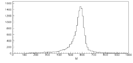
Figure 2: Invariant mass ($M$) distribution of the muon-jet pair in a dimuon-dijet sample for $m_{\tilde{t}_{1}}=600$ GeV. See text for details.

One can sharpen the signal further by constructing the invariant mass of the jet-lepton pair. In Ref. [22] the reconstruction of the stop mass from the signal events in a particular channel was illustrated. This is, however, possible even without $b$-tagging. Suppose we take the two hardest jets in an event and combine each of them with the two hard isolated leptons in turn, and keep only those events where both the invariant masses are close. The result is shown in Fig. 2 where the difference between two jet-lepton invariant masses is taken to be 20 GeV or less. We show the unnormalized distribution of invariant mass of the higher-mass muon-jet pair in the dimuon-dijet sample for $m_{\tilde{t}_{1}}=600$ GeV. This procedure can be used to further reduce the SM backgrounds, if necessary.

4 Analysis

In this section we will discuss the APS in the framework of the model as defined in Section 2 vis-à-vis the neutrino data. Apart from the RPV parameters, the neutrino masses and mixing angles depend on several RPC parameters. The tree-level contributions, as shown in Eqs. (2) and (3), depend on the combination $C$. As noted earlier, for a bino dominated $\tilde{\chi}^{0}_{1}$ and a wino dominated ${\tilde{\chi}}_{1}^{\pm}$, $C$ is naturally negative, or $C^{\prime}$ is naturally positive. Similarly, the one-loop contributions shown in Eq. (5) depend on the SU(2) gauge coupling, the trilinear soft breaking term $A_{b}$, $\mu$, $\tan\beta$, and the average $b$-squark mass ${m_{\tilde{b}}}$. The sign of the parameter $K$ defined in Eq. (5) depend on the relative magnitude and sign of $A_{b}$ and $\mu$. Note that the second term in Eq. (5) does not involve any further RPC parameters other than those already defined.

As said earlier, we assume, in the entire analysis, (i) the first two squark generations to be much heavier than the third, and (ii) bino-dominated $\tilde{\chi}^{0}_{1}$ and wino-dominated $\tilde{\chi}^{+}_{1}$.

The numerical inputs are

$$\mu=1.762~{}{\rm TeV}\,,\ \ \tan\beta=10\,,\ \ A_{t}=3~{}{\rm TeV}\,,\ \ A_{b}=-5.5~{}{\rm TeV}\,,\ \ m_{\tilde{b}}=2.5~{}{\rm TeV}\,,\ \ M_{2}-M_{1}=100~{}{\rm GeV}\,.$$ (9)

Apart from this, we take $m_{\tilde{\chi}^{0}_{1}}-m_{\tilde{t}_{1}}=25$ GeV for the stop LSP case, and $m_{\tilde{t}_{1}}-m_{\tilde{\chi}^{0}_{1}}=25$ and 75 GeV for stop NLSP cases. While $M_{1}$ is more or less fixed by the $\tilde{\chi}^{0}_{1}$ mass, $M_{2}$ is kept close to $M_{1}$ so that $C^{\prime}$ in Eq. (3) is large, which, as we will show, is favored by the neutrino data.

The stop decay width depends on the mixing angle $\theta_{t}$ defined in Eq. (7). This angle (as well as $m_{\tilde{t}_{1}}$) is computed from the $2\times 2$ stop mass matrix ${\cal M}^{\tilde{t}}$. We take the diagonal and off-diagonal entries of ${\cal M}^{\tilde{t}}$ as free parameters. The off-diagonal entries are proportional to the stop mixing parameter $X_{t}=A_{t}-\mu\cot\beta$; this has to be large so that the mass of the lighter Higgs scalar comes out to be in the range $126\pm 3$ GeV [27]. This motivates the choice of $A_{t}$. ${\cal M}^{\tilde{t}}_{LL}$, which is the common mass parameter for L-type stop and sbottom squarks, is chosen to be large so that the average sbottom mass is 2.5 TeV. Thus the relatively small ${\cal M}^{\tilde{t}}_{RR}$ essentially determines $m_{\tilde{t}_{1}}$, and this is the parameter that we tune to generate different $m_{\tilde{t}_{1}}$. Over the entire range of $m_{\tilde{t}_{1}}$ corresponding to observable signals, the allowed values of $\theta_{t}$ lie in a narrow range: $0.10\leq\cos\theta_{t}\leq 0.12$, which is due to the Higgs mass constraint. Thus, $\tilde{t}_{1}$ is dominantly $\tilde{t}_{R}$, but even the small $\tilde{t}_{L}$ component makes the RPV channels competitive to the RPC ones for stop NLSP case. The mixing angle is of no consequence for stop decays when $\tilde{t}_{1}$ is the LSP.

Given the above RPC parameters the solutions consistent with the neutrino masses and mixing depend on the interplay of the three biliear RPV parameters $\mu_{i}$ and the three trilinear couplings $\lambda^{\prime}_{i33}$. We randomly generate these parameters varying them over a wide range:

$$\mu_{i}\in[10^{-4},5\times 10^{-2}]~{}{\rm GeV}\,,\ \ \lambda^{\prime}_{i33}\in[2\times 10^{-8},2.5\times 10^{-4}]\,.$$ (10)

The required parameters are directly read from the SLHA output file generated by SUSPECT [28]. We choose only those points that satisfy all the neutrino constraints and correctly reproduce the Higgs mass $m_{h}$ in the allowed region.

The generated mass squared differences and mixing angles must be consistent with the neutrino oscillation data [24]. At $1\sigma$ level, this reads:

$$\Delta m_{21}^{2}=\left(7.45^{+0.19}_{-0.16}\right)\times 10^{-5}~{}{\rm eV}^{2}\,,\ \ \Delta m_{31}^{2}=(2.417\pm 0.014)\times 10^{-3}~{}{\rm eV}^{2}\,,$$

$$\sin^{2}(\theta_{12})=0.306\pm 0.012\,,\ \ \sin^{2}(\theta_{23})=(0.446\pm 0.008)\oplus 0.593^{+0.027}_{-0.043}\,,$$

$$\sin^{2}(\theta_{13})=0.0231\pm 0.0019\,.$$ (11)

However, the precise determination of $\sin^{2}\theta_{13}$ has severely constrained the parameter space for RPV models. The highly restrictive nature of the neutrino data can be understood from the fact that we hardly find any solutions from $10^{9}$ randomly generated points over the RPV parameter space as shown in Eq. (11). Therefore, we extend the range to $3\sigma$ level [24] for further analysis :

$$\Delta m_{21}^{2}=[6.98:8.05]\times 10^{-5}~{}{\rm eV}^{2}\,,\ \ \Delta m_{31}^{2}=[2.247:2.623]\times 10^{-3}~{}{\rm eV}^{2}\,,$$

$$\sin^{2}(\theta_{12})=[0.271:0.346]\,,\ \ \sin^{2}(\theta_{23})=[0.366:0.663]\,,\ \ \sin^{2}(\theta_{13})=[0.0173:0.0288]\,.$$ (12)

The combinations of the RPV parameters which are filtered through the above data defines the APS and each member of this set is refered to as a solution. We also require that the sum of all the neutrino masses must also satisfy

$$\sum m_{\nu}<0.22~{}{\rm eV~{}at~{}95\%~{}CL}\,$$ (13)

using the data from cosmic microwave background, the baryon acoustic oscillation, and the supernova luminosity distance from Hubble space telescope [29].

The values of $\lambda^{\prime}_{i33}$, for every solution, show a hierarchical structure; one or two of the couplings will be large compared to the other(s). This was also noted in Refs. [20] and [22]. Obviously, the number of any particular type of lepton in the final state is directly proportional to the square of the RPV coupling. Thus, all possible solutions can be divided into several groups, depending upon which lepton(s) are going to be dominant. For example, if $\lambda^{\prime}_{233}\gg\lambda^{\prime}_{133},\lambda^{\prime}_{333}$, we will expect only muon signals from such models. While there are nine possible leptonic combinations from the two stops, it reduces to only three for us ($ee$, $\mu\mu$, and $e\mu$) as we do not simulate final states with $\tau$, for reasons discussed before. Let us also note here that the solutions are almost equally spread about $\sin^{2}\theta_{23}=0.5$.

As we will show, for higher stop masses, some solutions are ‘lost’, i.e. the corresponding PBRs in all three dilepton channels ($ee$, $\mu\mu$ and $e\mu$) fall below the respective MOPBRs. One might wonder whether $\tau$ detection might help, although this possibility cannot be checked as yet for reasons already discussed. The pattern of the solutions, however, shows that for every stop mass (both LSP and NLSP cases), at least 50% of the solutions have $\lambda^{\prime}_{333}>\lambda^{\prime}_{133},\lambda^{\prime}_{233}$. Thus a significant fraction of the so-called ‘lost’ solutions may be observed through the $\tau$ channels. For example, with $m_{\tilde{t}_{1}}=900$ GeV for the stop LSP case and an integrated luminosity of 100 fb^-1, 144 solutions are lost, out of which $\lambda^{\prime}_{333}$ is largest for 112 solutions. For stop NLSP case, there are 188 (219) lost solutions with $m_{\tilde{t}_{1}}=700$ (900) GeV and $m_{\tilde{t}_{1}}-m_{\tilde{\chi}^{0}_{1}}=75$ GeV; 111 (114) of them have $\lambda^{\prime}_{333}$ as the largest coupling. Of course, just the fact that $\lambda^{\prime}_{333}$ is largest does not guarantee a detection through the $\tau$ channel.

4.1 ${\tilde{t}_{1}}$ LSP

In this subsection we study the APS for models where $\tilde{t}_{1}$ is the LSP and decays entirely through the RPV channels. For our parameter choice, $C^{\prime}$ (Eq. (3)) is positive but $K$ (Eq. (5)) is negative; for example,

$$C^{\prime}=1.2\times 10^{8}~{}{\rm eV}\,,\ \ K=-1.7\times 10^{6}~{}{\rm eV}\,,$$ (14)

for $m_{\tilde{t}_{1}}=600$ GeV. Note that changing the sign of $\mu$ would flip the sign of $K$ but $C^{\prime}$ is independent of sgn($\mu$). Later in the paper, we try to play with these constants , and it turns out that the above choice is close to the optimal one; no matter how we change the coefficients, the number of models that pass the neutrino data filter never has a order-of-magnitude enhancement. In almost all the cases, it goes down, and sometime goes down rather drastically.

Only the RPV channels are open for $\tilde{t}_{1}$ decay, and for each solution the BR of $\tilde{t}_{1}\to\ell_{i}+b$ is simply proportional to $\left({\lambda^{\prime}_{i33}}\right)^{2}$. The BRs are independent of $m_{\tilde{t}_{1}}$ and $\theta_{t}$; the dependence cancels out only for the stop LSP case.

$m_{\tilde{t}_{1}}$ (GeV)	No. of	$N_{ee}$	$N_{\mu\mu}$	$N_{e\mu}$	Lost
	solutions $N$				solutions $N_{0}$
500	348	73 (104)	309 (319)	239 (260)	0 (0)
550	306	48 (59)	272 (275)	176 (209)	0 (0)
600	250	41 (43)	219 (224)	105 (136)	1 (0)
650	247	40 (41)	200 (204)	92 (132)	10 (2)
700	251	46 (50)	186 (199)	64 (111)	17 (7)
750	238	31 (32)	161 (191)	35 (73)	48 (17)
800	233	17 (25)	141 (169)	6 (41)	75 (40)
850	222	14 (19)	109 (136)	0 (11)	99 (67)
900	223	8 (20)	70 (104)	1 (1)	144 (99)
950	203	0 (6)	5 (63)	0 (0)	198 (134)
1000	199	0 (0)	0 (0)	0 (0)	199 (199)

Table 1: Distribution of signals for the various model solutions. Column 2 shows the total number of solutions $N$; columns 3-5 show the solutions that result in an observable $ee$, $\mu\mu$, or $e\mu$ signal (PBR $>P^{\rm min}_{ij}$). The last column shows the number of ‘lost’ solutions $N_{0}$ for which no signal can be observed. The numbers are for ${\cal L}=100(300)$ fb^-1.

Table 1 summarizes our result for this case. The second column gives, for different $m_{\tilde{t}_{1}}$, the number of solutions $N$ after scanning over $10^{9}$ randomly generated combinations. This is only indicative of the stringent nature of the neutrino data; $N$ will increase if we employ a finer scan, focussing around individual solutions. This number might be contrasted with [22], where a few thousand solutions were obtained for the same number of randomly generated points in spite of imposing a tighter constraint of taking the neutrino data at the $2\sigma$ level.

It is a bit puzzling to note that $N$, which is apparently independent of $m_{\tilde{t}_{1}}$, decreases significantly for higher values of $m_{\tilde{t}_{1}}$. This is due to the fact that in this case $M_{1}$ and $M_{2}$ must also be large to maintain the stop LSP condition. As a result, $C^{\prime}$ in Eq. (3) goes down while $K$ remains unchanged, thereby reducing the probability of satisfying the constraints from neutrino data. For higher values of $M_{1}$ and/or $M_{2}-M_{1}$, the number of solutions goes down in general.

Our process is the production of a $\tilde{t}_{1}$ pair and its subsequent decay to a pair of leptons plus $b$-jets. There are only three leptonic channels ($ee$, $\mu\mu$ and $e\mu$) that we focus upon; for each of these channels, the number of solutions $N_{\ell\ell}$ for which the signal is above the MOPBR limit is shown in the next three columns of Table 1. The numbers are shown for integrated luminosities of 100 and 300 fb^-1 respectively, the latter within parentheses. In the last column, we show the number of ‘lost’ solutions, denoted by $N_{0}$.

Note that $N_{0}$ increases with $m_{\tilde{t}_{1}}$; we lose almost half of the solutions for $m_{\tilde{t}_{1}}>850$ GeV with 100 fb^-1 and $m_{\tilde{t}_{1}}>900$ GeV with 300 fb^-1. The higher luminosity option is of marginal help, as we have noted before. Above $m_{\tilde{t}_{1}}=950$ GeV, we do not expect to see the signals for any solution point. However, $\tau$ detection might be of considerable help.

4.2 $\tilde{t}_{1}$ NLSP

As discussed in the introduction, for a $\tilde{t}_{1}$ NLSP with $m_{\tilde{t}_{1}}>m_{\tilde{\chi}^{0}_{1}}$, there may be various competing RPC decay modes of $\tilde{t}_{1}$ depending on the parameter space. These modes are: (i) $\tilde{t}_{1}\to t\tilde{\chi}^{0}_{1}$, which is not kinematically allowed if $m_{\tilde{t}_{1}}-m_{\tilde{\chi}^{0}_{1}}<m_{t}$, (ii) $\tilde{t}_{1}\to bW\tilde{\chi}^{0}_{1}$, which may be dynamically suppressed if LSP is almost a pure bino, (iii) $\tilde{t}_{1}\to c\tilde{\chi}^{0}_{1}$, which is a loop-induced process, and (iv) $\tilde{t}_{1}\to f\bar{f}^{\prime}b\tilde{\chi}^{0}_{1}$. The process (ii) swamps the RPV decay channels when $m_{\tilde{t}_{1}}-m_{\tilde{\chi}^{0}_{1}}>m_{W}$ and if the RPV couplings are of the order of $10^{-4}$–$10^{-5}$. Thus, we restrict ourselves to two typical cases: $m_{\tilde{t}_{1}}-m_{\tilde{\chi}^{0}_{1}}=25$ and 75 GeV, keeping $m_{\tilde{t}_{1}}$ a free parameter. Thus only processes (iii) and (iv) may possibly be the competing RPC decay channels.

$m_{\tilde{t}_{1}}$ (GeV)	$m_{\tilde{\chi}^{0}_{1}}$ (GeV)	BR (RPV)	No. of	$N_{ee}$	$N_{\mu\mu}$	$N_{e\mu}$	Missed
		(%)	solutions $N$				solutions $N_{0}$
500	425	6 - 53	410	53 (59)	266 (317)	49 (82)	97 (44)
	475	64 - 96	384	68 (85)	337 (344)	230 (248)	1 (0)
550	475	7 - 55	388	36 (51)	174 (251)	33 (74)	191 (89)
	525	64 - 97	348	66 (71)	299 (306)	198 (230)	2 (2)
600	525	7 - 57	329	16 (33)	101 (188)	15 (39)	215 (121)
	575	65 - 97	299	48 (51)	249 (260)	120 (167)	10 (1)
650	575	8 - 63	269	17 (23)	52 (77)	2 (18)	200 (173)
	625	61 - 97	250	36 (41)	207 (219)	65 (99)	12 (1)
700	625	6 - 69	256	19 (21)	50 (67)	0 (4)	188 (168)
	675	63 - 97	247	37 (41)	184 (203)	59 (99)	28 (7)
750	675	8 - 68	238	13 (14)	39 (51)	0 (5)	187 (173)
	725	63 - 98	251	39 (47)	161 (185)	28 (72)	52 (19)
800	725	8 - 72	241	8 (16)	38 (58)	0 (0)	195 (168)
	775	65 - 98	225	20 (24)	133 (158)	5 (37)	71 (45)
850	775	6 - 72	238	2 (7)	16 (43)	0 (0)	223 (188)
	825	66 - 98	233	13 (17)	102 (133)	0 (3)	119 (83)
900	825	8 - 74	219	0 (2)	0 (21)	0 (0)	219 (196)
	875	69 - 98	222	6 (11)	59 (93)	0 (0)	157 (118)
950	875	8 - 74	223	0 (0)	0 (0)	0 (0)	223 (223)
	925	64 - 99	223	0 (6)	2 (58)	0 (0)	221 (159)
1000	925	8 - 81	212	0 (0)	0 (0)	0 (0)	212 (212)
	975	67 - 98	203	0 (0)	0 (0)	0 (0)	203 (203)

Table 2: Same as Table 1 but for the stop NLSP case. For each stop mass, two cases are shown where the LSP $\tilde{\chi}^{0}_{1}$ is 25 (75) GeV below $m_{\tilde{t}_{1}}$. The branching fractions for both stops decaying through RPV channels are also shown. The numbers are for ${\cal L}=100(300)$ fb^-1.

The RPC parameters are fixed as before. For a given stop mass, the stop mixing angle $\theta_{t}$ is no longer a constant like the LSP case, because of the presence of RPC channels. However, $\cos\theta_{t}$ still remains small, almost at about the same range as in the LSP case.

Our results are shown in Table 2, which is similar to Table 1, except that the second column shows the LSP mass and the third column shows the BR of the stop through RPV channels. The remaining columns 4–8 carry the same information as colums 2–6 of Table 1.

Several points are to be noted here. First, $N$ is fairly insensitive to $m_{\tilde{t}_{1}}-m_{\tilde{\chi}^{0}_{1}}$ for fixed $m_{\tilde{t}_{1}}$. However, $N$ decreases with increasing $m_{\tilde{t}_{1}}$ for reasons discussed in the last subsection. Second, the probability of RPV decays (by which we mean both the $\tilde{t}_{1}$s will decay to $\ell+b$) goes down with increasing $m_{\tilde{t}_{1}}-m_{\tilde{\chi}^{0}_{1}}$, and this is true for all values of $m_{\tilde{t}_{1}}$. This is because the RPC channels start to open up with increasing phase space. Third, the ‘reach’ for the stop NLSP case is in general a bit lower compared to the stop LSP case, which is again due to the dilution of the RPV branching fractions from the RPC channels.

4.3 Parameter variation

In this subsection we vary some of the key RPC parameters individually, keeping others fixed. The rationale is to check whether our choice is the optimal or close to optimal one, or whether there exists some other benchmark with allows a significantly larger number of solutions. Of course the RPV parameters $\mu_{i}$ and $\lambda^{\prime}_{i33}$ are generated randomly and scanned over their entire range. We show the entire variation for $m_{\tilde{t}_{1}}=600$ GeV. For the stop NLSP case, we display results only for $m_{\tilde{t}_{1}}-m_{\tilde{\chi}^{0}_{1}}=25$ GeV. In all tables in this subsection, the first numerical columns represent our benchmark scenario, followed by the variations.

4.3.1 Variation of $\mu$

Table 3 shows the effect of changing $\mu$ by $\pm 500$ GeV from our benchmark of 1762 GeV. While the number of solutions increase (decrease) for lower (higher) values of $\mu$, the change is not so drastic. One might wonder why there should be a variation at all, as the tree-level neutrino mass matrix depends on the ratios $\mu_{i}/\mu$ and $\mu_{j}/\mu$. However, $\mu$ also appears in the first term of Eq. (5) in a nontrivial way, and the interplay determines the number of solutions.

$\mu$ (GeV)	1762	1262	2262
No. of	299	618	260
solutions	(250)	(614)	(248)

Table 3: Variation of $\mu$. We show the number of solutions in $10^{9}$ tries that pass the neutrino filter. The numbers in parentheses are for the stop LSP case.

4.3.2 Variation of $M_{2}-M_{1}$

The results are shown in Table 4. Note that there is only a modest change of N as we vary our benchmark mass difference of 100 GeV. However, low values of $M_{2}-M_{1}$, which increase $C^{\prime}$, help towards more solutions.

$(M_{2}-M_{1})$ (GeV)	100	300	500
No. of	299	232	219
solutions	(250)	(239)	(221)

Table 4: Variation of $M_{2}-M_{1}$. The numbers in parentheses are for the stop LSP case.

4.3.3 Variation of average bottom squark mass

Entries in $M^{\lambda^{\prime}\lambda^{\prime}}$ are inversely proportional to $m^{2}_{\tilde{b}}$, and those in $M^{\mu\lambda^{\prime}}$ are inversely proportional to $m_{\tilde{b}}$, the average $b$-squark mass. The number of solutions decrease when $m_{\tilde{b}}$ goes down. When $m_{\tilde{b}}$ is increased, the behavior is different for $\tilde{t}_{1}$ LSP and NLSP cases, but the number of solutions remain at the same order of magnitude. Thus, our choice of $m_{\tilde{b}}$ is optimal for stop NLSP and close to optimal for stop LSP case. For the NLSP case, smaller $m_{\tilde{b}}$ enforces smaller $\lambda^{\prime}_{i33}$ to generate the same solutions, so the RPV BRs also go down.

$m_{\tilde{b}}$ (GeV)	2500	1500	3000
No. of	299	70	200
solutions	(250)	(109)	(499)

Table 5: Variation of $m_{\tilde{b}}$. The numbers in parentheses are for the stop LSP case.

4.3.4 Variation of $C^{\prime}$ and $K$

Next, we vary the parameters $C^{\prime}$ in Eq. (3) and $K$ in Eq. (5), one at a time. We see from Table 6 that our choice of $C^{\prime}$ is the optimal one; both the allowed number of solutions and the RPV branching ratios fall as we move by one order of magnitude to either side. Note that the variation of $C^{\prime}$ affects only the tree-level mass term, unlike the variation of $\mu$, which affects all terms. Also, the relative values of $C^{\prime}$ and $K$ are important to generate correct atmospheric as well as solar splittings. Identical conclusions appear from the variation of $K$, see Table 7, where we have shown our results also by flipping the sign of $\mu$. Even though we have not considered the variation of the $\mu_{i}\lambda^{\prime}_{i33}$ term, this exercise alone shows that the neutrino mass hierarchy is strongly preferred to be a normal one.

$C^{\prime}$ (eV)	$1.2\times 10^{8}$	$1.2\times 10^{7}$	$1.2\times 10^{9}$
No. of	299	115	8
solutions	(250)	(107)	(11)

Table 6: Variation of the tree-level coefficient $C^{\prime}$ of the neutrino mass matrix. The numbers in parentheses are for the stop LSP case.

$K$ (eV)	$-1.7\times 10^{6}$	$-1.7\times 10^{5}$	$-1.7\times 10^{7}$	$8.9\times 10^{5}$
No. of	299	114	9	99
solutions	(250)	(2)	(10)	(83)

Table 7: Variation of the loop-level coefficient $K$ of the neutrino mass matrix. The numbers in parentheses are for the stop LSP case. The last column is when the sign of $\mu$ is flipped: $\mu=-1762$ GeV.

Before we end, let us mention that the rotation from $\{H_{2},L_{i}\}$ basis to $\{H^{\prime}_{2},L^{\prime}_{i}\}$ basis can in principle induce charged lepton-chargino, and neutrino-neutralino mixing. They can affect the decays of the NLSP, $\tilde{t}_{1}$, or the LSP, $\tilde{\chi}^{0}_{1}$. For example the RPC vertex $\tilde{t}_{1}$–$b$–chargino may lead to additional lepton number violating couplings of the $\tilde{t}_{1}$ due to chargino-lepton mixings. Similar induced couplings may arise from $\tilde{t}_{1}$–$t$–neutralino coupling due to mixing in the neutralino-neutrino sector (these couplings may be relevant only if the $\tilde{t}_{1}$ is significantly heavier than the top quark). The mixing factors which would suppress the induced couplings can be estimated from the 5 $\times$ 5 (7 $\times$ 7) chargino-lepton (neutralino-neutrino) mass matrix. The estimated value is ${\cal O}(\mu_{i}/\mu)\sim 10^{-7}$. Since the largest $\mu_{i}$ allowed by the oscillation data is ${\cal O}(10^{-4})$ GeV, the mixing factors are estimated to be ${\cal O}(10^{-7})$ or smaller. Moreover, the induced couplings will be additionally suppressed by gauge or Yukawa couplings. On the other hand the smallest $\lambda^{\prime}_{i33}$ coupling contributing to $\tilde{t}_{1}$ decay consistent with the nuetrino oscillation data is ${\cal O}(10^{-5})$. Thus the $\tilde{t}_{1}$-NLSP BRs computed by considering $\lambda^{\prime}_{i33}$ driven decays only are quite reliable.

We now justify the above estimates by some numerical results, analogous to those obtained in [21]. We numerically diagonalize the mass matrices in the chargino-lepton or the neutralino-neutrino sector for all combinations of RPV parameters allowed by the oscillation data. We find that the chargino-charged lepton mixing is always extremely tiny; A typical amplitude for finding a charge lepton mass eigenstate in a chargino is $1.6\times 10^{-6}$. The corresponding $\lambda^{\prime}_{133}$, responsible for the $\tilde{t}_{1}$ or LSP decay signal, is $1.2\times 10^{-4}$. Similarly the maximum amplitude for finding a neutrino mass eigenstate in any neutralino is $1.5\times 10^{-6}$. The corresponding $\lambda^{\prime}_{133}$ is $1.2\times 10^{-4}$. The above results are for $m_{{\tilde{\chi}}_{1}^{0}}=500$ GeV but this trend is seen over the entire range of parameters considered in this paper.

5 Summary

In conclusion, we reiterate that the current neutrino data severely constrain the RPV generated neutrino mass models. In this paper, we have discussed a particular type of such models, where the neutrino mass matrix is generated by three bilinear and three trilinear $\lambda^{\prime}_{i33}$-type couplings. The severity of the constraint can be gauged from the fact that out of a billion randomly generated sets of the above six parameters, only a few hundred at the most are found to be consistent with the data. While the actual number of solutions depends on the RPC parameters, we have explicitly checked that our choice of those parameters is close to optimal. We have intentionally refrained from making an absolute optimal choice of the RPC parameters, just to keep our analysis on the conservative side. We have also kept our analysis on the conservative side, by considering only electrons and muons in the final state, and not employing $b$-tagging, as $\tau$- and $b$-tagging efficiencies at LHC-14 TeV are not yet publicly available. Even with such a conservative analysis, we get a lot of interesting conclusions.

The model considered in this paper may be tested through the RPV decays of the lighter stop squark, $\tilde{t}_{1}$, provided it is the LSP or the NLSP. These scenarios with a relatively light $\tilde{t}_{1}$ are now well motivated since the mixing parameter $X_{t}$ in the stop sector is likely to be large in view of the measured value of $m_{h}\approx$ 126 GeV, resulting in a rather light stop mass eigenstate. For a stop pair produced at LHC-14 TeV, we consider their RPV decays into the channels $\ell_{i}\ell_{j}+2$ jets. Using PYTHIA based simulations, we obtain model independent estimates of the minimum observable product branching ratios as a function of $m_{\tilde{t}_{1}}$. In contrast to an earlier work by two of us, we show that a favourable signal may be obtained without $b$-tagging. Following this procedure one can also reconstruct the mass of $\tilde{t}_{1}$ from the lepton-jet invariant mass distributions, which in turn reveals the lepton number violating nature of the underlying stop decays.

We then consider the RPV models consistent with neutrino data and compute the product branching ratios for each of them. We find that for lower values of $m_{\tilde{t}_{1}}$, signals from almost all the models are observable; on the other hand, the fraction of observable models goes down with increasing $m_{\tilde{t}_{1}}$, and for $m_{\tilde{t}_{1}}$ around 1 TeV, no signal can be seen for any of the allowed models. We have checked that many of the lost solutions correspond to $\lambda^{\prime}_{333}>\lambda^{\prime}_{133},\,\lambda^{\prime}_{233}$, especially for moderately heavy $\tilde{t}_{1}$. Once the techniques for handling $\tau$ rich final states at LHC-14 TeV experiments and the corresponding background estimates are available, the inclusion of these states will improve the observability of neutrino mass models.

6 Acknowledgements

R.B. acknowledges Council for Scientific and Industrial Research, Govt. of India, and A.K. acknowledges Department of Science and Technology, Govt. of India, and Council for Scientific and Industrial Research, Govt. of India for research support. A.D acknowledges the award of an emeritus Senior Scientist Position by the Indian National Science Academy.

References

-
[1]
S. Schael et al. [ALEPH and DELPHI and L3 and OPAL and SLD and LEP
Electroweak Working Group and SLD Electroweak Group and SLD Heavy Flavour
Group Collaborations],
Phys. Rept. 427, 257 (2006)
[hep-ex/0509008];
M. Baak et al., Eur. Phys. J. C 72, 2205 (2012) [arXiv:1209.2716 [hep-ph]]. -
[2]
G. Aad et al. [ATLAS Collaboration],
Phys. Lett. B 716, 1 (2012)
[arXiv:1207.7214 [hep-ex]];
G. Aad et al. [ATLAS Collaboration], Phys. Rev. D 86, 032003 (2012) [arXiv:1207.0319 [hep-ex]]. - [3] S. Chatrchyan et al. [CMS Collaboration], Phys. Lett. B 716, 30 (2012) [arXiv:1207.7235 [hep-ex]].
-
[4]
See, e.g. R. N. Mohapatra and P. B. Pal, Massive Neutrinos in Physics
and Astrophysics, World Scientific, Singapore, 2004;
The review on neutrino mass and mixing in the Particle Data Group webpage (2013 update) at http://pdg.lbl.gov/2013/reviews/rpp2013-rev-neutrino-mixing.pdf, and the webpage http://www.nu-fit.org for the latest numbers. - [5] See any standard review on Higgs physics, e.g. L. Reina, hep-ph/0512377.
- [6] For reviews on Supersymmetry, see, e.g. H. P. Nilles, Phys. Rept. 1, 110 ( 1984); H. E. Haber and G. Kane, Phys. Rept. 117, 75 ( 1985) ; J. Wess and J. Bagger, Supersymmetry and Supergravity, 2nd ed., (Princeton, 1991); M. Drees, P. Roy and R. M. Godbole, Theory and Phenomenology of Sparticles, (World Scientific, Singapore, 2005).
- [7] G. Jungman, M. Kamionkowski and K. Griest, Phys. Rept. 267, 195 (1996) [hep-ph/9506380].
- [8] For reviews on RPV SUSY see, e.g. H. K. Dreiner, in Kane, G.L. (ed.): Perspectives on supersymmetry II, pp. 565-583 [hep-ph/9707435]; M. Chemtob, Prog. Part. Nucl. Phys. 54, 71 (2005) [hep-ph/0406029].
- [9] R. Barbier, C. Berat, M. Besancon, M. Chemtob, A. Deandrea, E. Dudas, P. Fayet and S. Lavignac et al., Phys. Rept. 420, 1 (2005) [hep-ph/0406039];
- [10] For a review, see S. Rakshit, Mod. Phys. Lett. A 19, 2239 (2004) [hep-ph/0406168]. See Ref. [15] of this review for detailed references.
-
[11]
For various neutrino mass generation mechanisms through RPV, see, e.g.
Y. Grossman and H. E. Haber, Phys. Rev. Lett. 78, 3438 (1997) [hep-ph/9702421]; S. Davidson, M. Losada and N. Rius, Nucl. Phys. B 587, 118 (2000) [hep-ph/9911317]; S. Davidson and M. Losada, JHEP 0005, 021 (2000) [hep-ph/0005080]; Phys. Rev. D 65, 075025 (2002) [hep-ph/0010325]; F. Borzumati and J. S. Lee, Phys. Rev. D 66, 115012 (2002) [hep-ph/0207184]; Y. Grossman and S. Rakshit, Phys. Rev. D 69, 093002 (2004) [hep-ph/0311310]. Also see Ref. [15] of [10]. -
[12]
A. S. Joshipura and M. Nowakowski,
Phys. Rev. D 51, 2421 (1995)
[hep-ph/9408224];
M. Nowakowski and A. Pilaftsis, Nucl. Phys. B 461, 19 (1996) [hep-ph/9508271];
A. S. Joshipura and S. K. Vempati, Phys. Rev. D 60, 111303 (1999) [hep-ph/9903435];
J. C. Romao, M. A. Diaz, M. Hirsch, W. Porod and J. W. FValle, Phys. Rev. D 61, 071703 (2000) [hep-ph/9907499];
M. Hirsch, M. A. Diaz, W. Porod, J. C. Romao and J. W. F. Valle, Phys. Rev. D 62, 113008 (2000) [Erratum-ibid. D 65, 119901 (2002)] [hep-ph/0004115];
A. Abada, S. Davidson and M. Losada, Phys. Rev. D 65, 075010 (2002) [hep-ph/0111332];
A. Datta, J. P. Saha, A. Kundu and A. Samanta, Phys. Rev. D 72, 055007 (2005) [hep-ph/0507311];
M. A. Diaz, M. Hirsch, W. Porod, J. C. Romao and J. W. F. Valle, Phys. Rev. D 68, 013009 (2003) [Erratum-ibid. D 71, 059904 (2005)] [hep-ph/0302021];
Y. Grossman and S. Rakshit, Phys. Rev. D 69, 093002 (2004) [hep-ph/0311310];
B. C. Allanach and C. H. Kom, JHEP 0804, 081 (2008) [arXiv:0712.0852 [hep-ph]];
Z. Marshall, B. A. Ovrut, A. Purves and S. Spinner, arXiv:1402.5434 [hep-ph]. -
[13]
A. Abada and M. Losada,
Phys. Lett. B 492, 310 (2000)
[hep-ph/0007041];
A. Abada, G. Bhattacharyya and M. Losada, Phys. Rev. D 66, 071701 (2002) [hep-ph/0208009]. -
[14]
A. Datta and B. Mukhopadhyaya,
Phys. Rev. Lett. 85, 248 (2000)
[hep-ph/0003174];
D. Restrepo, W. Porod and J. W. F. Valle, Phys. Rev. D 64, 055011 (2001) [hep-ph/0104040]. - [15] D. Acosta et al. [CDF Collaboration], Phys. Rev. Lett. 92, 051803 (2004) [hep-ex/0305010].
- [16] S. Chakrabarti, M. Guchait and N. K. Mondal, Phys. Rev. D 68, 015005 (2003) [hep-ph/0301248]; Phys. Lett. B 600, 231 (2004) [hep-ph/0404261].
- [17] S. P. Das, A. Datta and M. Guchait, Phys. Rev. D 70, 015009 (2004) [hep-ph/0309168].
- [18] K. -i. Hikasa and M. Kobayashi, Phys. Rev. D 36, 724 (1987).
- [19] C. Boehm, A. Djouadi and Y. Mambrini, Phys. Rev. D 61, 095006 (2000) [hep-ph/9907428].
- [20] S. P. Das, A. Datta and S. Poddar, Phys. Rev. D 73, 075014 (2006) [hep-ph/0509171].
- [21] A. Datta and S. Poddar, Phys. Rev. D 75, 075013 (2007) [hep-ph/0611074].
- [22] A. Datta and S. Poddar, Phys. Rev. D 79, 075021 (2009) [arXiv:0901.1619 [hep-ph]].
- [23] T. Sjostrand, P. Eden, C. Friberg, L. Lonnblad, G. Miu, S. Mrenna and E. Norrbin, Comput. Phys. Commun. 135, 238 (2001) [hep-ph/0010017]; for a more recent version, T. Sjostrand, S. Mrenna and P. Z. Skands, JHEP 0605, 026 (2006) [hep-ph/0603175].
- [24] The fit webpage, at http://www.nu-fit.org.
- [25] S. Chatrchyan et al. [CMS Collaboration], Phys. Rev. Lett. 110, 081801 (2013) [arXiv:1210.5629 [hep-ex]].
- [26] A. Kundu and J. P. Saha, Phys. Rev. D 70, 096002 (2004) [hep-ph/0403154].
-
[27]
G. Degrassi, S. Heinemeyer, W. Hollik, P. Slavich and G. Weiglein,
Eur. Phys. J. C 28, 133 (2003)
[hep-ph/0212020];
B. C. Allanach, A. Djouadi, J. L. Kneur, W. Porod and P. Slavich, JHEP 0409, 044 (2004) [hep-ph/0406166];
S. P. Martin, Phys. Rev. D 75, 055005 (2007) [hep-ph/0701051];
R. V. Harlander, P. Kant, L. Mihaila and M. Steinhauser, Phys. Rev. Lett. 100, 191602 (2008) [Phys. Rev. Lett. 101, 039901 (2008)] [arXiv:0803.0672 [hep-ph]];
S. Heinemeyer, O. Stal and G. Weiglein, Phys. Lett. B 710, 201 (2012) [arXiv:1112.3026 [hep-ph]];
A. Arbey, M. Battaglia, A. Djouadi and F. Mahmoudi, JHEP 1209, 107 (2012) [arXiv:1207.1348 [hep-ph]]. - [28] A. Djouadi, J. -L. Kneur and G. Moultaka, Comput. Phys. Commun. 176, 426 (2007) [hep-ph/0211331]; we use version 2.43.
- [29] E. Giusarma, E. Di Valentino, M. Lattanzi, A. Melchiorri and O. Mena, arXiv:1403.4852 [astro-ph.CO].