Deep ocean early warning signals of an Atlantic MOC collapse

Qing Yi Feng, Jan P. Viebahn and Henk A. Dijkstra

Institute for Marine and Atmospheric research Utrecht (IMAU),

Department of Physics and Astronomy, Utrecht University, Utrecht, The Netherlands.

The Atlantic Meridional Overturning Circulation (MOC) is a crucial part of the climate system because of its associated northward heat transport [1, 2]. The present-day MOC is sensitive to freshwater anomalies and may collapse to a state with a strongly reduced northward heat transport [3, 4]. A future collapse of the Atlantic MOC has been identified as one of the most dangerous tipping points in the climate system [7]. It is therefore crucial to develop early warning indicators for such a potential collapse based on relatively short time series. So far, attempts to use indicators based on critical slowdown have been marginally successful [8]. Based on complex climate network reconstruction [9, 10], we here present a promising new indicator for the MOC collapse that efficiently monitors spatial changes in deep ocean circulation. Through our analysis of the performance of this indicator we formulate optimal locations of measurement of the MOC to provide early warning signals of a collapse. Our results imply that an increase in spatial resolution of the Atlantic MOC observations (i.e., at more sections) can improve early detection, because the spatial coherence in the deep ocean arising near the transition is better captured.

To develop this indicator and to study its performance, we use the results from the control simulation and the freshwater perturbed (from now on referred to as ‘hosing’) simulation of the FAMOUS climate model (see Methods). In the hosing simulation, the freshwater flux over the extratropical North Atlantic is increased linearly from zero to 1.0 Sv (1 Sv = 10⁶ m³s^-1) over 2000 years [11]. Fig. 1a displays the annual mean time series of the Atlantic MOC value at latitude 26^∘N and at 1000 m depth for the control simulation (green curve) and the hosing simulation (blue curve). Whereas the control MOC values are statistically stationary over the 2000 year integration period, the MOC values for the hosing simulation show a rapid decrease between the years 800-1050.

We also use results from the FAMOUS simulations in which the freshwater flux was fixed after a certain integration time and the model was integrated to equilibrium [11]. Time series of the MOC of the last 100 years of these simulations were analyzed and the mean MOC values (again at 26^∘N and 1000 m depth) are plotted as the red dots labeled from 1 to 6 in Fig. 1a. Figure 1b-d show mean MOC streamfunction patterns of three of these equilibrium simulations (labelled with 1, 4 and 6 in Fig. 1a). Although the equilibrium value of the MOC decreases with larger freshwater inflow, the changes in the MOC pattern are relatively minor.

For a slightly higher value of the freshwater flux as at point 6, the equilibrium solution is already a collapsed state [11]. In the hosing simulation, the freshwater is, however, added relatively fast compared to the equilibration time scale of the MOC. Hence the MOC maintains its pattern for much higher freshwater inflow and collapses near year 900 (Fig. 1a). To determine a collapse time $\tau_{c}$ more precisely, we use the control simulation of FAMOUS (see Methods). We find $\tau_{c}=874$ years and $\tau_{c}$ is shown as the red dashed line in Fig. 1a.

Critical slowdown has been a key phrase in the detection of tipping points in ecosystems [12] and the climate system [8]. Indeed in many natural and man-made systems, there is an increase in response times to perturbations as a tipping point is approached [13]. The detection of MOC collapses and the design of early warning signals has so far mostly been based on the analysis of single time series [14, 8]. Critical slowdown induces changes in variance and lag-1 autocorrelation in the time series that can be connected to the distance to the tipping point and hence these quantities can serve as early warning indicators [13].

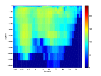
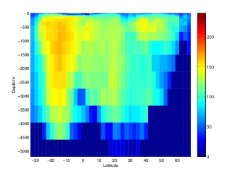
(a) (b)

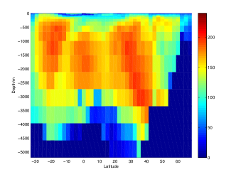
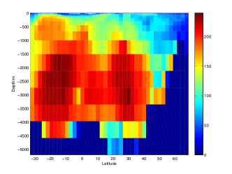
(c) (d)

Figure 2: (a) Degree field of the Pearson Correlation Climate Network (PCCN) constructed from the MOC data of equilibrium simulation 1 in Fig. 1a using a threshold $\tau=0.5$. (b) Same as (a) but of equilibrium simulation 2. (c) Same as (a) but of equilibrium simulation 4. (d) Same as (a) of equilibrium simulation 6.

Here we build on an idea to use complex network theory to construct an early warning indicator [15]. The complex network we employ in this study is the Pearson Correlation Climate Network [17] abbreviated below as PCCN (see Methods for details on the network reconstruction). We first construct PCCNs using the complete Atlantic MOC field for each of the six 100 year equilibrium simulations (red dots in Fig. 1a). For the topological analysis of the PCCNs, we only use the degree field [9, 10, 18]. The degree of a node is the number of links between this node and other nodes. As shown in Fig. 2 the changes in the degree field at the equilibrium solutions 1, 2, 4 and 6 in Fig. 1a are distinct. When the freshwater forcing is increased, high degree in the network – indicating high spatial MOC correlations – first appears at nodes in the South Atlantic at about 1000 m depth (Fig. 2a-b). It subsequently extends to the whole Atlantic with highest amplitudes in the deep ocean at midlatitudes (Fig. 2c-d).

A similar result was obtained using networks from the temperature field of an idealized spatially two-dimensional model of the MOC [15]. The behavior of the degree field can be understood from the underlying structure of the Empirical Orthogonal Functions (EOFs) of the MOC field (see Supplementary Information). Once the transition is approached, one of the EOFs becomes most dominant in the variability. The network can be seen as a coarse-graining of the variability and by focussing only on the largest correlations, it is ideally suited to monitor the changes in spatial correlations of the system once the transition is approached.

Next, we study the transient behavior of the hosing simulation by constructing similar PCCNs (see Methods for details on the sliding window and threshold values $\tau$ used). In [15], the kurtosis $K_{d}$ of the degree distribution was introduced as an effective indicator to capture the changes in the topology of the degree field. For the complete Atlantic MOC field, the values of $K_{d}$ for the hosing simulation (blue curve) and for the control simulation (green curve) are plotted in Fig. 3a. For the hosing simulation, there is indeed a strong increase of $K_{d}$ to values far extending those for the control simulation significantly before the collapse time $\tau_{c}$. For comparison, the critical slowdown indicators variance (Fig. 3b) and lag-1 autocorrelation (Fig. 3c) based on the complete Atlantic MOC data (and using the same sliding window) do not show any early warning signal of the MOC transition before the collapse time $\tau_{c}$.

To provide a measure of the performance of an indicator $I$, we introduce an evaluation scheme (see Methods), which consists of the detection time, the reliability of the indication, and the intensity of the indication, $\gamma^{I}$. The excellent performance of the kurtosis indicator ${K_{d}}$ (with a detection time at 738 years, no false alarm and a positive value of $\gamma^{K_{d}}$) in Fig. 3a is shown in entry No.1 in Table 1.

So far, we used the complete Atlantic MOC field of the FAMOUS model data, but at the moment, MOC observations are only routinely made at 26^∘N through the RAPID-MOCHA program [19]. There are also initiatives to monitor the MOC at 35^∘S (SAMOC, see www.aoml.noaa.gov/phod/SAMOC_international) and at about 60^∘N (OSNAP, see www.o-snap.org). Motivated by the fact that current and near future available observations of the MOC will only be available along zonal sections in the Atlantic, we next reconstructed networks (and the indicator $K_{d}$) from limited section MOC data of the FAMOUS model results.

The performance of the kurtosis indicator ${K_{d}}$ for different sections and combinations of sections is shown in Table 1. The indicator $K_{d}$ provides two false alarms (see Methods) and one relatively late alarm for data at 26^∘N (No. 2 in Table 1), no alarm at all for data at 33^∘S (No. 3 in Table 1) and does not perform well for all other single section data (see Supplementary Table 1). When the lag-1 autocorrelation and variance of time series averaged over a single section are considered (see Supplementary Tables 2 and 3), the lag-1 autocorrelation performs best at 21^∘N although it still gives a false alarm. The variance indicator does not give any warning for all single sections.

To determine the optimal observation locations of the MOC using $K_{d}$, we systematically deleted sections from the complete Atlantic MOC field and evaluated the performance of the indicator $K_{d}$ for the remaining sections. Entry No. 4 in Table 1 shows that the indicator $K_{d}$ still works well for the Atlantic MOC field with halved horizontal resolution (21(depth) $\times$ 21(latitude)$=441$ nodes), as well as for the sets of sections including midlatitudes both in the Northern and Southern Hemisphere (No. 6-8 in Table  1). However, detection fails for the set of sections located only in the Northern Hemisphere at mid- and high latitudes (No. 5 in Table 1).

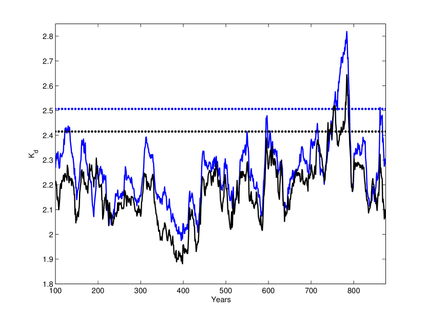
Figure 4: The kurtosis indicator $K_{d}$ for section data constructed from 21 depth levels and 8 latitudes. (a) Data from 31^∘N, 26^∘N, 21^∘N, 16^∘N, 11^∘N, 8^∘S, 13^∘S and 18^∘S (blue solid curve), gives the early warning signal at 753 years and lasts for 38 years. (b) Data from 31^∘N, 26^∘N, 21^∘N, 16^∘N, 11^∘N, 13^∘S, 18^∘S and 33^∘S (black solid curve), gives the early warning signal at 740 years and lasts for 49 years. The dotted blue horizontal line indicates the maximum $K_{d}$ value of the control simulation of section data (a), and the dotted black horizontal line indicates the corresponding maximum $K_{d}$ value of section data (b).

For the latitude sets I and II, consisting of 18^∘S, 13^∘S, 8^∘S, 11^∘N, 16^∘N, 21^∘N, 26^∘N and 31^∘N (blue curve in Fig. 4 and No. 9 in Table 1) or 33^∘S, 18^∘S, 13^∘S, 11^∘N, 16^∘N, 21^∘N, 26^∘N and 31^∘N (green curve in Fig. 4 and No. 10 in Table 1), respectively, the performance of the indicator $K_{d}$ is comparable to the case of the complete Atlantic MOC field (Fig. 3a and No. 1 in Table 1). Both sets consist of 21(depth)$\times$8(latitude)$=168$ grid points and hence are considerably reduced (by 81%) in comparison to the complete Atlantic MOC field. Further analysis (see Supplementary Table 4) indicates that the data at the sections 18^∘S and 31^∘N are essential for a good detection of the MOC collapse. The results of No. 9 and 10 in Table  1 also indicate that including the MOC data at 33^∘S (near the SAMOC section) would advance the detection time of a future collapse of the MOC compared to including a section at 8^∘S, but the detection intensity $\gamma^{K_{d}}$ of the kurtosis indicator ${K_{d}}$ slightly decreases.

The physical reason for the optimal observation regions is the following. In ocean-climate models, the MOC collapse is due to a robust feedback involving the transport of salinity by the ocean circulation, the salt-advection feedback [5, 6]. The subtropics are strong evaporation regions and hence the largest salinity gradients, central in the salt-advection feedback, are located in these regions. Consequently, it is expected that here the strongest response due to the salt-advection feedback appears and hence the strongest spatial correlations in the MOC field. Support for this comes from the structure of the dominant EOFs of the equilibrium solutions where the largest amplitude is also located in these midlatitude regions (see Supplementary Material).

Using techniques of complex network theory we have provided a novel indicator which can give an early warning signal for a collapse of the MOC. When applied to data from the FAMOUS model [11], our results show that when the appropriate midlatitude North and South Atlantic MOC data are available, the kurtosis indicator $K_{d}$ provides a strong anomalous signal at least 100 years before the transition. Although at the moment a collapse of the MOC is considered a high-impact but low-probability event [20], modesty is required regarding our confidence in this statement. The processes controlling the behavior of the MOC, such as the downwelling in the northern North Atlantic boundary currents, are not well represented in many of the climate models on which this statement is based. In state-of-the-art GCMs, such as those used in the IPCC AR5, MOC collapses have not been found yet but it is fair to say that these models have not been extensively tested for this behavior [20, 21].

Up to now, there is about 10 years of data on the MOC from the RAPID-MOCHA array, and although this array will likely be operational up to the year 2020, the temporal extend of the time series proceeds only slowly. Due to this insufficient length of the observational record, the indicator $K_{d}$ is not yet applicable to observational data and hence cannot be used to determine whether the recent downward trend in the observed MOC strength at 26^∘N [22] is the start of a collapse. Such MOC behavior may just be related to natural variability such as that associated with the Atlantic Multidecadal Oscillation [23, 24]. The strong element of an indicator such as $K_{d}$ is, however, that it is based in spatial correlations. Our results indicate that an increase in spatial resolution of the MOC observations (i.e., at more sections) can improve early detection using this indicator, because the spatial coherence arising near the transition is better captured. This is another reason that such observations should be given high priority in climate research.

Methods

• Model: The FAMOUS model is a version of the HadCM3 model with a lower resolution ocean and atmosphere component; the details of the model are described in [11]. The model has horizontal resolution of 2.5^∘ $\times$ 3.75^∘ and a vertical resolution of 20 levels. Annual mean data of the MOC field were analyzed for each simulation.

• Collapse Time $\tau_{c}$: With a Student t-test we first determine the time, say $\tau_{s}$, at which the trend of the MOC time series of the hosing simulation deviates significantly (p = 0.05) from that of the control simulation. Subsequently, the standard deviation $\sigma$ of the MOC values of the control simulation over the first $\tau_{s}$ years is computed. Next, the first time when the MOC anomaly value (with respect to the mean of the first $\tau_{s}$ years) in the hosing simulation decreases below - 3$\sigma$, we consider the MOC to start collapsing which defines $\tau_{c}$. In the FAMOUS model, when considering the MOC values at 26^∘N and 1000 m depth, we find $\tau_{s}=$ 350 years and $\tau_{c}=$ 874 years.

• Network Reconstruction: From the MOC data of the FAMOUS model over the latitudinal domain [35^∘S-70^∘N] of the Atlantic Ocean, we construct a Climate Network (CN). The nodes of the network are the latitude-depth values of the grid points of the model. A ‘link’ between two nodes is determined by a significant interdependence between their MOC anomaly time series. There are several measures of quantifying the degree of statistical interdependence, and the most common one is calculating the Pearson correlations of pairs of time series [16]. More precisely, in a Pearson Correlation Climate Network (PCCN) [17] an unweighted and undirected link between two nodes exists if the linear Pearson correlation coefficient of the MOC time series at these two nodes exceeds a threshold value such that the correlation is significant (p=0.05).

  For example, in case of the complete Atlantic MOC field and the 100 year equilibrium simulations, each network consists of 21(depth) $\times$ 42 (latitude)$=882$ nodes, and a threshold value of $\tau=0.5$ guarantees that a Pearson correlation between MOC time series at two nodes exceeding $\tau$ is significant. For the hosing simulation, as shown in Fig. 1a, the MOC values display a significant trend which would affect the accuracy of early warning signal detection. Hence, for the study of the transient behaviour of the hosing simulation, we first linearly detrend the MOC field before reconstruction of the PCCNs. Next, a 100-year sliding window size (with a shift of one year) is used and values of $\tau$ between 0.5 and 0.9 are chosen for each PCCN, which guarantees significant correlations (p = 0.05) in defining the links among the nodes in each PCCN.

• Evaluation Scheme for the Performance of an Indicator:
  1) Detection time: When a value of an indicator for the hosing simulation exceeds the maximum of the same indicator for the control simulation, we flag an alarm of a collapse. For example, the maximum of $K_{d}$ for the control simulation (green curve in Fig. 3a) is plotted as the blue dashed line in Fig. 3a. In this case, an early warning signal is detected at year 738 which is 136 years before the MOC collapse time $\tau_{c}=874$ years.
  2) False Alarm: We label a detection time which is smaller than $\tau_{c}-300$ years as a false alarm. The 300 years is based on the horizon considered in IPCC-AR5 [20] for the evolution of the climate system (such as reflected in the Extended Concentration Pathway Emissions and Forcing scenarios, ECPs). Such a time period is also considered to be a political time horizon [7] such that decisions taken within this period are able to affect the occurrence of a collapse. In addition, when the detection time is within [$\tau_{c}-300,\tau_{c}$], but the signal only lasts less than 5 years it is also considered as a false alarm.
  3) Detection intensity $\gamma^{I}$: The amplitude of the peak of the indicator is also important. Therefore, we additionally define another quality measure $\gamma^{I}$ for indicator $I$ as

  $$\gamma^{I}=\frac{\max_{P}(I^{hosing})}{\max_{[0,\tau_{c}]}(I^{control})}-1$$

  Here the maximum of the control is taken over the total time interval $[0,\tau_{c}]$ and that of the hosing only over the peak interval $P$ where the indicator extends over the threshold value. The larger the value of $\gamma^{I}$ the better the quality of the indicator $I$; if $\gamma^{I}\leq 0$ no detection occurs. For example, based on the results in Fig. 3a the value of $\gamma^{K_{d}}$ for the complete Atlantic MOC field is about 0.07 (see No. 1 in Table 1). Values of $\gamma$ for both the variance (Fig. 3b) and the lag-1 autocorrelation (Fig. 3c) are smaller than zero.

Correspondence

Correspondence and requests for materials should be addressed to Q. Y. Feng (email: Q.Feng@uu.nl).

Author contribution

All three authors designed the study, Q. Y. Feng performed most of the analysis, and all authors contributed to the writing of the paper.

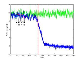
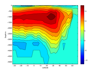
(a) (b)

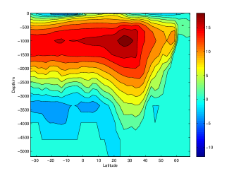
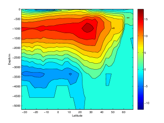
(c) (d)

Figure 1: (a) Time series of the MOC (in Sv, 1 Sv = 10⁶ m³s^-1) at 26^∘N and 1000m depth in the Atlantic for the control simulation (green curve) and the freshwater perturbed simulation (blue curve) of the FAMOUS model. The red dots labeled from 1 to 6 show the average values of MOC from the corresponding equilibrium simulations and the red broken line indicates the collapse time $\tau_{c}=874$ years. (b) Annual mean MOC streamfunction pattern of equilibrium simulation 1. (c) Same as (b) but of equilibrium simulation 4. (d) Same as (b) but of equilibrium simulation 6.

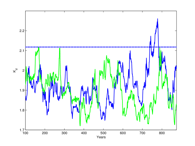
(a)

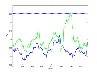
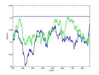
(b) (c)

Figure 3: For the complete Atlantic MOC field, (a) the kurtosis indicator $K_{d}$ gives the early warning signal at 738 years and lasts for 44 years. (b) The traditional variance indicator Var gives no early warning signal before the collapse time $\tau_{c}=874$ years. (c) The traditional lag-1 autocorrelation indicator Autocorr gives no early warning signal before the collapse time $\tau_{c}$. Green solid curves are related to the control simulation and blue solid curves are related to the hosing simulation. The dashed blue horizontal lines indicate the corresponding maximum values of the control simulation.

Table 1: The performance of the kurtosis indicator $K_{d}$ based on complex networks constructed from sets of section data at different latitudes. In the sets of sections indicated by brackets, the first entry indicates the southern boundary, the second entry the northern boundary and the third entry is the latitudinal step.

No.	Section	Detection Time (Year)	False Alarm	$\gamma^{K_{d}}$
1	(35∘S, 70∘N, 2.5∘)	738	No	0.0675
2	26∘N	384/567/868	Yes/Yes/No	0.1031/0.0451/0.0105
3	33∘S	-	-	-0.1252
4	(35∘S, 70∘N, 5∘)	739	No	0.0472
5	(20∘N, 70∘N, 5∘)	-	-	0
6	(35∘S, 20∘N, 5∘)	785	No	0.0559
7	(35∘S, 35∘N, 5∘)	785	No	0.0773
8	(20∘S, 35∘N, 5∘)	785	No	0.0584
9	Latitude set I	753	No	0.1248
10	Latitudes set II	740	No	0.0951
11	Latitude set III	-	-	-0.0810
12	Latitude set IV	-	-	-0.0454

1. : 18^∘S, 13^∘S, 8^∘S, 11^∘N, 16^∘N, 21^∘N, 26^∘N and 31^∘N

2. : 33^∘S, 18^∘S, 13^∘S, 11^∘N, 16^∘N, 21^∘N, 26^∘N and 31^∘N

3. : 13^∘N, 16^∘N, 18^∘NS, 21^∘N, 23^∘N, 26^∘N, 28^∘N and 31^∘N

4. : 33^∘S, 31^∘S, 28^∘S, 26^∘S, 23^∘S, 21^∘S, 18^∘S and 16^∘S

References

- [1] Ganachaud, A. & Wunsch, C. Improved estimates of global ocean circulation, heat transport and mixing from hydrographic data. Nature 408, 453–457 (2000).
- [2] Johns, W., Baringer, M. & Beal, L. Continuous, array-based estimates of Atlantic Ocean heat transport at 26.5 N. Journal Of Climate 24, 2429–2449 (2011).
- [3] Bryan, F. O. High-latitude salinity effects and interhemispheric thermohaline circulations. Nature 323, 301–304 (1986).
- [4] Rahmstorf, S. The thermohaline circulation: a system with dangerous thresholds? Climatic Change 46, 247–256 (2000).
- [5] Stommel, H. Thermohaline convection with two stable regimes of flow. Tellus 2, 244–230 (1961).
- [6] Walin, G. The thermohaline circulation and the control of ice ages. Paleogeogr. Paleoclim. Paleoecol. 50, 323–332 (1985).
- [7] Lenton, T. M. et al. Tipping elements in the earth’s climate system. Proceedings of the National Academy of Sciences 105, 1786–1793 (2008).
- [8] Lenton, T. M. Early warning of climate tipping points. Nature Publishing Group 1, 201–209 (2011).
- [9] Tsonis, A. A. & Swanson, K. L. What do networks have to do with climate? Bulletin Of The American Meteorological Society 87, 585–595 (2006).
- [10] Donges, J. F., Zou, Y., Marwan, N. & Kurths, J. Complex networks in climate dynamics. The European Physical Journal Special Topics 174, 157–179 (2009).
- [11] Hawkins, E. et al. Bistability of the Atlantic overturning circulation in a global climate model and links to ocean freshwater transport. Geophysical Research Letters 38, L10605 (2011).
- [12] Dakos, V., Kéfi, S., Rietkerk, M., van Nes, E. H. & Scheffer, M. Slowing down in spatially patterned ecosystems at the brink of collapse. The American Naturalist 177, 154–166 (2011).
- [13] Scheffer, M., Bascompte, J., Brock, W. A. & Brovkin, V. Early-warning signals for critical transitions. Nature 461, 53–59 (2009).
- [14] Livina, V. N. & Lenton, T. M. A modified method for detecting incipient bifurcations in a dynamical system. Geophysical Research Letters 34 (2007).
- [15] Mheen, M. et al. Interaction network based early warning indicators for the Atlantic MOC collapse. Geophysical Research Letters 40, 2714–2719 (2013).
- [16] Tsonis, A. A. & Roebber, P. J. The architecture of the climate network. Physica A: Statistical Mechanics and its Applications 333, 497–504 (2004).
- [17] Feng, Q. Y. & Dijkstra, H. Are North Atlantic multidecadal SST anomalies westward propagating? Geophysical Research Letters 41, 541–546 (2014).
- [18] Viebahn, J. & Dijkstra, H. A. Critical Transition Analysis of the Deterministic Wind-Driven Ocean Circulation — A Flux-Based Network Approach. International Journal of Bifurcation and Chaos 24, 1430007 (2014).
- [19] Cunningham, S. A. et al. Temporal Variability of the Atlantic Meridional Overturning Circulation at 26.5 N. Science 317, 935–938 (2007).
- [20] Collins, M. et al. Long-term Climate Change: Projections, Commitments and Irreversibility. In Stocker, T. et al. (eds.) Climate Change 2013: The Physical Science Basis. Contribution of Working Group I to the Fifth Assessment Report of the Intergovernmental Panel on Climate Change, 1029–1136 (Cambridge: University of Cambridge Press Syndicate., UK, 2013).
- [21] Huisman, S. E., den Toom, M., Dijkstra, H. A. & Drijfhout, S. An Indicator of the Multiple Equilibria Regime of the Atlantic Meridional Overturning Circulation. Journal Of Physical Oceanography 40, 551–567 (2010).
- [22] Smeed, D. A. et al. Observed decline of the atlantic meridional overturning circulation 2004 to 2012. Ocean Science Discussions 10, 1619–1645 (2013). URL http://www.ocean-sci-discuss.net/10/1619/2013/.
- [23] Kerr, R. A. A North Atlantic climate pacemaker for the centuries. Science 288, 1984–1986 (2000).
- [24] Knight, J. R., Allan, R. J., Folland, C. K., Vellinga, M. & Mann, M. E. A signature of persistent natural thermohaline circulation cycles in observed climate. Geophysical Research Letters 32, L20708 (2005).
(a)
(b)
(b)
(c)
(d)
(d)
(a)
(b)
(b)
(c)
(d)
(d)
(a)
(b)
(c)
(c)