Super-luminous supernovae from PESSTO

Abstract

We present optical spectra and light curves for three hydrogen-poor super-luminous supernovae followed by the Public ESO Spectroscopic Survey of Transient Objects (PESSTO). Time series spectroscopy from a few days after maximum light to 100 days later shows them to be fairly typical of this class, with spectra dominated by Ca II, Mg II, Fe II and Si II, which evolve slowly over most of the post-peak photospheric phase. We determine bolometric light curves and apply simple fitting tools, based on the diffusion of energy input by magnetar spin-down, ⁵⁶Ni decay, and collision of the ejecta with an opaque circumstellar shell. We investigate how the heterogeneous light curves of our sample (combined with others from the literature) can help to constrain the possible mechanisms behind these events. We have followed these events to beyond 100-200 days after peak, to disentangle host galaxy light from fading supernova flux and to differentiate between the models, which predict diverse behaviour at this phase. Models powered by radioactivity require unrealistic parameters to reproduce the observed light curves, as found by previous studies. Both magnetar heating and circumstellar interaction still appear to be viable candidates. A large diversity is emerging in observed tail-phase luminosities, with magnetar models failing in some cases to predict the rapid drop in flux. This would suggest either that magnetars are not responsible, or that the X-ray flux from the magnetar wind is not fully trapped. The light curve of one object shows a distinct re-brightening at around 100d after maximum light. We argue that this could result either from multiple shells of circumstellar material, or from a magnetar ionisation front breaking out of the ejecta.

1 Introduction

In recent years, observational studies of supernovae (SNe) have been revolutionized by a new generation of transient surveys, which observe large areas of the sky without a bias for particular galaxy types. The Palomar Transient Factory (PTF; Rau et al., 2009), Pan-STARRS1 (PS1; Kaiser et al., 2010), Catalina Real-Time Transient Survey (CRTS; Drake et al., 2009), and La Silla QUEST (LSQ; Baltay et al., 2013), for example, find thousands of SNe per year, among which lurk some very unusual objects. In particular, there has been much interest in a population of very luminous blue transients inhabiting faint galaxies. Quimby et al. (2011) were the first to obtain secure measurements of their redshifts, and establish these SNe as a new class, through detections of narrow host galaxy Mg II $\lambda$$\lambda$ 2796, 2803 absorption lines. Typical redshifts $z\sim$ 0.2–0.5 implied absolute peak magnitudes $M<-21$, making these SNe at least 10–100 times more luminous than the usual thermonuclear (type Ia) and core-collapse SNe. This intrinsic brightness enabled Pan-STARRS1 to extend the redshift range to $z\sim 1$ (Chomiuk et al., 2011). Cooke et al. (2012) have since detected events as distant as $z\sim 2$ and 4, in stacked images from the Canada-France-Hawaii Telescope Legacy Survey Deep Fields.

Gal-Yam (2012) reviewed these “super-luminous” supernovae (SLSNe), and defined three sub-classes, roughly in analogy with conventional SN nomenclature. The hydrogen-rich events were named SLSNe II. Many of these show narrow and intermediate-width Balmer emission lines, similar to normal SNe IIn, and their light curves are likely powered by a collision between the SN ejecta and a massive, optically thick circumstellar shell (Smith & McCray, 2007; Smith et al., 2008; Miller et al., 2009; Benetti et al., 2014). In this case, kinetic energy is thermalised in the opaque shell by radiation-dominated shocks (Chevalier & Irwin, 2011), and diffuses out as observable light. The archetypal example of this class is SN 2006gy (Smith et al., 2007; Ofek et al., 2007).

The group identified by Quimby et al. (2011) were designated as SLSNe of Type I, since they are hydrogen-poor. The first examples were SN 2005ap (Quimby et al., 2007) and SCP-06F6 (Barbary et al., 2009). The early optical spectra of these objects are dominated by broad absorptions of O II, and are very blue and quite featureless around peak brightness. Pastorello et al. (2010) showed that a relatively nearby object, SN 2010gx, evolved to spectroscopically resemble more typical SNe Ic, but with delayed line formation relative to their normal-luminosity cousins (also see Chen et al., 2013, for late-time, and host galaxy, analysis). The mechanism that powers SLSN I or Ic remains undetermined. However, it is clear that the light curves observed so far are incompatible with models powered by the radioactive decay chain ⁵⁶Ni—⁵⁶Co—⁵⁶Fe (Quimby et al., 2011; Gal-Yam, 2012; Inserra et al., 2013), which is the usual energy source in Type Ia or Ibc SNe. One plausible candidate is delayed heating by a central engine, such as a spinning-down magnetar (Woosley, 2010; Kasen & Bildsten, 2010; Dessart et al., 2012) or fall-back accretion (Dexter & Kasen, 2013), giving luminous light curves with power-law declines. Another possibility is circumstellar interaction with hydrogen-free shells (Woosley, Blinnikov & Heger, 2007); however, it has not been shown whether this can produce the observed spectra, which lack narrow lines. Inserra et al. (2013) collected extensive data on 5 SLSNe of Type Ic (in their nomenclature) at redshift $z<0.25$. They found that magnetar models could quantitatively reproduce the observed light curves.

The third sub-class is based on the decline rate of the SN luminosity. A small number of hydrogen-free SLSNe have light curve gradients after peak magnitude which are consistent with radioactive ⁵⁶Co decay. This led Gal-Yam (2012) to propose a classification name of SLSN-R. These may be the observational counterparts of the long-predicted pair-instability supernovae (PISNe; Barkat, Rakavy & Sack, 1967; Rakavy & Shaviv, 1967). In these models, photons in the cores of 130–250 M_⊙ stars are sufficiently energetic to decay into electron-positron pairs, and the conversion of pressure-supporting radiation to rest-mass triggers contraction followed by thermonuclear runaway. Only one published event, SN 2007bi (Gal-Yam et al., 2009; Young et al., 2010), has been considered a strong candidate for a PISN. However, two very similar SLSNe, PTF12dam and PS1-11ap, with better photometric and spectroscopic coverage, have since been shown by Nicholl et al. (2013) and McCrum et al. (2014) to be inconsistent with PISN models, and their early spectra resemble the other SLSNe Ic. Whether or not the fast (2005ap-like) and slowly decaying (2007bi-like) SLSNe are powered by the same mechanism, and whether there are two distinct classes or a continuum of events, remains to be seen.

A related phenomenon is the “pulsational pair-instability” (Woosley, Blinnikov & Heger, 2007) in stars of 65–130 M_⊙. In this case, the energy released by explosive burning, following pair-production, is less than the binding energy of the star. Many solar masses of material may be ejected before the star resumes stable burning, and the instability may be encountered several times before a normal core-collapse SN terminates its life. This is a promising means of producing circumstellar shells (H-rich or -poor) in interaction models of SLSNe. No definitive objects of this type have been identified, but Ben-Ami et al. (2014) have presented SN 2010mb, an energetic SN Ic (though not technically super-luminous) with an extremely extended light curve and narrow oxygen emission lines, and their analysis gave strong evidence for a SN interacting with hydrogen-free circumstellar material, matching predictions of pulsational-PISN models.

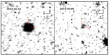
Figure 1: NTT+EFOSC2 $V$-band images of LSQ12dlf (200s; left) and a faint, extended source at the SN location, likely to be the host galaxy (18$\times$200s; right).

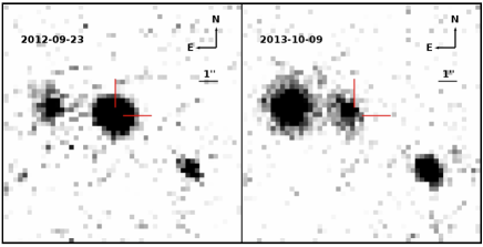
Figure 2: NTT+EFOSC2 $R$-band images of SSS120810 (60s; left) and its host galaxy (18$\times$200s; right). The SN is offset $\sim 0.\arcsec 5$ from the centre of the host.

The Public ESO Spectroscopic Survey of Transient Objects (PESSTO; Smartt et al. (2014); Smartt et al., in prep) aims to classify and follow up hundreds of young and unusual SNe, including those of the super-luminous variety, using primarily the European Southern Observatory (ESO) 3.58m New Technology Telescope (NTT) and EFOSC2 spectrograph (Buzzoni et al., 1984). These spectra are publicly available on WISeREP (Weizmann Interactive Supernova data REPository; Yaron & Gal-Yam, 2012). PESSTO provides a unique opportunity in the study of these rare objects, since the survey strategy is naturally geared towards classifying young objects and guaranteeing follow-up spectra with good time-sampling. In this paper, we report observations and modelling of three SLSNe Ic discovered during the first year of PESSTO: LSQ12dlf, SSS120810:231802-560926, and SN 2013dg, and also apply our models to PTF12dam (Nicholl et al., 2013), SN 2011ke (Inserra et al., 2013), and the SLSN II, CSS121015:004244+132827 (Benetti et al., 2014). In section 2, we describe the discovery and classification of each SN. Section 3 presents and discusses their spectra, while section 4 does the same for the light curves. We have developed a suite of light curve fitting tools, which we outline in section 5; these models are then applied in section 6. We summarize our findings in section 7.

2 Discovery and classification

2.1 LSQ12dlf

LSQ12dlf was identified as a hostless transient by the La Silla QUEST Variability Survey (LSQ; Baltay et al., 2013), using the ESO 1.0m Schmidt Telescope, on 2012 July 10.4 UT, at RA=01:50:29.8, Dec=-21:48:45.4 (all coordinates in this paper are given in J2000.0). A spectrum obtained by PESSTO with NTT+EFOSC2, on 2012 Aug 08.3 UT, showed it to be a SLSN Ic about 10 days after peak luminosity. Comparison with SN 2010gx, and the other members of the PESSTO SLSN sample, indicated a redshift $z\approx 0.25$ (Inserra et al., 2012). No host galaxy emission or absorption lines are visible, even in a higher-resolution follow-up spectrum obtained with the Very Large Telescope (VLT)+X-Shooter (Vernet et al., 2011). To determine the redshift, we cross-correlated the X-shooter spectrum (which we found was at an epoch of +36d after maximum, see Section 3.2) with a spectrum of SN 2010gx at +29d (Pastorello et al., 2010). We found a minimum relative shift in the cross-correlation function for a redshift of $z=0.255\pm 0.005$. Deep EFOSC2 imaging on 2013 Oct 10.3 UT, $\sim$300 days after peak in the SN rest frame, and further follow-up in Jan-Feb 2014, showed a very faint host galaxy, with a magnitude $V\approx 25$ (Figure 1).

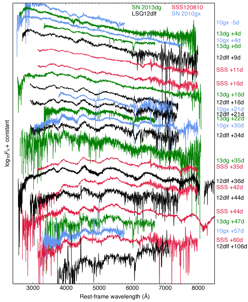
Figure 3: The spectral evolution of our three PESSTO SLSNe, compared to SN 2010gx, a well-observed SLSN Ic. The four SNe show virtually identical spectral evolution, dominated initially by blue continua, and then by broad lines of Ca II, Mg II, Fe II and Si II (see Fig. 4). Epochs (RHS) given in days from light curve peak, in the rest-frames of the SNe.

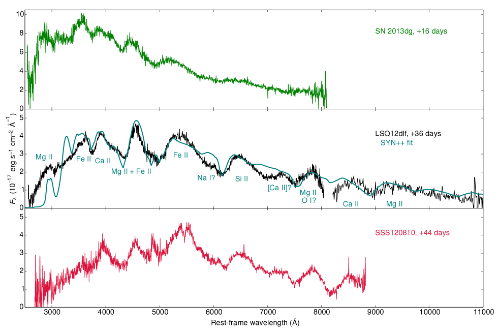
Figure 4: VLT+X-shooter spectra of our 3 SLSNe, at 2–6 weeks after maximum light (rest-frame). The data have been binned by 10 pixels to improve the signal-to-noise. Also shown is a synthetic spectrum, generated using SYN++ (Thomas, Nugent & Meza, 2011), used to identify the main line-forming ions. The best-fitting model spectrum has a photospheric velocity of $11000\,\rm{km}\,{s}^{-1}$, and temperature of 7000 K. We see that the spectra are dominated by singly-ionised intermediate-mass metals and iron.

2.2 SSS120810

SSS120810:231802-560926 (hereafter: SSS120810) was discovered by the Siding Spring Survey (SSS), a division of the Catalina Real-Time Transient Survey (Drake et al., 2009) with the 0.5m Uppsala Schmidt Telescope, on 2012 Aug 11.2. No host was present in SSS reference images at the location of the SN (RA=23:18:01.8, Dec=-56:09:25.6). PESSTO classified it on 2012 Aug 17–18 as a SLSN Ic, again roughly 10 days after maximum light (Inserra et al., 2012). The redshift was initially estimated as $z\approx 0.14-0.16$, from comparisons with other SLSNe Ic. A spectrum taken at +44d after peak with the VLT+X-shooter (see Section 3.2), showed a distinct, narrow emission line at 7587.5 Å, with a full-width-half-maximum of FWHM=9.4 Å. The line is resolved and is almost certainly H$\alpha$ at $z=0.156$. Unfortunately, this is right in the telluric A band, which compromises a definitive measurement of the flux and width. Assuming this redshift, the X-Shooter spectrum also shows weak and narrow lines at wavelengths corresponding to two other common host galaxy emission lines : [O II] $\lambda$ 3727 and [O III] $\lambda$ 5007. This gives confidence that the strongest narrow emission line is indeed H$\alpha$ at $z=0.156$ and we adopt this redshift for the supernova. Deep $BVRI$ imaging with EFOSC2 on 2012 Oct 10.1 and 25.0, $\sim$380 rest-frame days after peak, revealed a clear host galaxy, which is likely the source of the narrow emission lines. The SN is offset from the centre of this galaxy by $0.\arcsec 51\pm$0.04 (Fig. 2).

2.3 SN 2013dg

SN 2013dg was detected by the Mount Lemmon Survey (MLS) and Catalina Sky Survey (CSS), both of which are part of CRTS (Drake et al., 2009) . MLS initially discovered the transient, MLS130517:131841-070443, on 2013 May 17.7 UT with the 1.5m Mt. Lemmon Telescope, while CSS independently found it with the 0.68m CSS Schmidt Telescope on May 30.7 UT, giving the alternative designation CSS130530:131841-070443. The exact coordinates are RA=13:18:41.38 and Dec=-07:04:43.1. PESSTO identified MLS130517 as an interesting target, but could not take an EFOSC2 spectrum at this time, as the survey takes a break from May–July when the Galactic centre is over La Silla. We instead classified this object using the William Herschel Telescope (WHT) and ISIS spectrograph on 2013 Jun 11.0. The spectrum was dominated by a blue continuum, and resembled SLSNe Ic a few days after maximum light (Smartt et al., 2013). The WHT spectrum has two features that were identified as possible Mg II absorption, from either the host galaxy of SN 2013dg or intervening material, at a redshift of $z=0.192$ (Smartt et al., 2013). These are not visible in the X-shooter spectrum, but the signal-to-noise of the data at 3300 Å precludes a useful quantitative check. The features are at the correct separation if they were the Mg II $\lambda\lambda$ 2795.528, 2802.704 doublet, but the data are noisy, the lines are close to edge of the CCD and they can’t be confirmed as real. Nevertheless, this redshift is ruled out by the broad supernova features in the spectrum. We cross-correlated the X-shooter spectrum (which we found was at an epoch of +16d after maximum, see Section 3.2) with a spectrum of SN2010gx at +11d (Pastorello et al., 2010). We found a minimum relative shift in the cross-correlation function when we set $z=0.265\pm 0.005$. Hence we suspect the possible absorption is either not real or is foreground and we and adopt a redshift of $z=0.265\pm 0.005$ for the supernova. No host galaxy emission lines are visible in any of our spectra and the host is not detected in deep imaging taken 250 days after peak (in Feburary 2014) down to $r>25.6$.

3 Spectroscopy

3.1 Data aquisition and reduction

The majority of our spectroscopy was carried out within PESSTO, using NTT+EFOSC2. The data were reduced using our custom PESSTO pipeline (developed in python by S. Valenti), which calls standard iraf tasks through pyraf, to de-bias and flat-field the two-dimensional frames, and wavelength- and flux-calibrate the spectra using arc lamps and spectrophotometric standard stars, respectively. The spectra are cleaned of cosmic-ray contamination using lacosmic (Van Dokkum, 2001) before the 1D spectrum is extracted. The pipeline also uses a model to subtract telluric features (see Smartt et al. in prep).

Each of our SLSNe were also observed with VLT+X-Shooter. These data were reduced using the X-Shooter pipeline within ESO’s Reflex package. X-Shooter routinely observes telluric standard stars for all targets, and these were used to remove telluric features from our spectra within iraf. SN 2013dg was classified with WHT at the beginning of the PESSTO off-season, and additional spectra were obtained with GMOS on the Gemini South telescope (Hook et al., 2004). These were processed using standard iraf tasks in ccdproc and onedspec; GMOS spectra were extracted using the gemini package, while the WHT spectrum was extracted with apall. The details of all spectra can be found in Tables 2, 3 and 4.

3.2 Spectral evolution

The observed spectral evolution of our three objects is shown in Figure 3. All spectra have been corrected for redshift and Milky Way extinction, according to the recalibration of the infrared galactic dust maps by Schlafly & Finkbeiner (2011) ($E(B-V)=0.013;0.019;0.047$, for LSQ12dlf, SSS120810 and SN 2013dg, respectively). We assume negligible internal extinction, since narrow Na I D absorption features are always very weak or absent. All phases are given in days, in the SN rest-frame, from the date of maximum luminosity.

Between $\sim$10–60 days after peak, we have excellent time-series coverage of all three supernovae, which we compare to one of the most thoroughly observed SLSNe Ic, SN 2010gx (Pastorello et al., 2010). Our earliest spectrum is the WHT classification of SN 2013dg, obtained at 4 days after maximum light. At this phase, the spectra are dominated by a blue continuum with a blackbody temperature $T\sim 13000$K, with a few weak absorption features between 4000–5000 Å. These may be attributable to O II, which tends to dominate this region of SLSNe Ic spectra before and around peak, as can be seen in SN 2010gx. However, these lines seem to be at slightly redder wavelengths in SN 2013dg. It is possible that we have observed SN 2013dg during the transition from the O II–dominated early spectrum to the nearly-featureless spectrum (with broad, shallow iron lines) seen just after peak in SN 2010gx. This interpretation is supported by our GMOS spectrum, 2 days later, which closely resembles the first post-maximum spectrum of SN 2010gx. It should be noted, however, that radiative transfer models by Howell et al. (2013) instead favoured C II/III and Fe III as the dominant species in the early (around maximum light) spectra of some SLSNe.

The spectral evolution over days 10–60 is remarkably consistent across these four SNe. Our X-Shooter spectrum of LSQ12dlf, at 36 days after light curve maximum, is shown in Figure 4, along with a synthetic SYN++ spectrum for line identification (Thomas, Nugent & Meza, 2011). The spectrum is dominated by singly-ionised metals. The strongest lines in the optical are Ca II H&K, Mg II $\lambda$ 4481 (blended with Fe II), a broad Fe II feature between $\sim 4900-5500$ Å, and the Si II $\lambda$ 6350 doublet feature. Beyond a phase of $\sim$50 days, the peak of the feature around $\sim$4500 Å appears to move to slightly redder wavelength, suggesting Mg I] $\lambda$ 4571 emission is dominant. These are the same features identified by Inserra et al. (2013) in a sample of SLSNe Ic at similar redshifts.

The Fe II lines in the spectrum of LSQ12dlf are stronger and develop earlier than in the other objects of the sample, and are already quite pronounced less than 10 days after peak light. This is very similar to the behaviour of PTF11rks, in the Inserra et al. (2013) sample. That object also transitioned to resemble a normal SN Ic by this epoch, compared to the 20–30 days required in most SLSNe Ic. The authors suggested that this faster evolution could be related to its lower luminosity, relative to the other members of their sample. However, LSQ12dlf peaks at an absolute AB magnitude of $r\sim-21.4$, which is quite typical for SLSNe Ic, and in line with the rest of our sample, and in fact declines more slowly in luminosity than the other PESSTO objects (see Section 4).

The final spectrum of LSQ12dlf, 106 days after maximum light, was taken with GMOS. By this time, the SN has cooled to only a few thousand kelvin. The spectrum at this epoch seems to be dominated by a fairly red continuum (i.e. it has not reached the nebular phase), as well as the same broad lines of singly-ionized metals that have remained present throughout the observed lifetime of the SN. This latest spectrum may also show a weak Na I D absorption; however, given the low signal-to-noise, such an identification is not firm. The reddening is also present in our $k$-corrected photometry, which suggests $B-V\approx 0.04$ at 44 days after peak, and $B-V\approx 0.58$ at $\sim$100 days (the epochs of our last two spectra).

In the last spectrum of SSS120810, at 60 days, we do detect a weak Na I D line. The spectra of SSS120810 beyond 35 days all show some barely-resolved structure in the iron blends between $\sim$4500–5500 Å, matching that in SN 2011kf (Inserra et al., 2013). X-Shooter spectra of SSS120810 and LSQ12dlf extend the wavelength range into the near-infrared. We can see strong Mg II absorptions at around 7500 and 9000 Å, the former of which is probably blended with O I $\lambda$ 7775, and a clear Ca II NIR triplet. Overall, the spectral evolution of our objects seems to be much in line with the general picture of SLSNe Ic that has been emerging over the last few years.

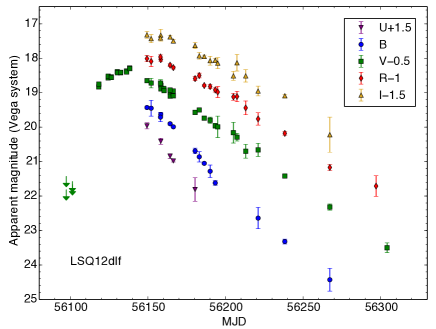
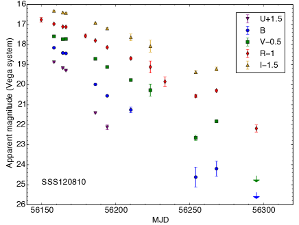
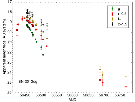
Figure 5: Multi-colour light curves of our SLSNe, in the observer frame

4 Photometry

4.1 Data aquisition and reduction

Imaging of our SLSNe came from a variety of sources. In addition to NTT+EFOSC2, we collected data with the 2m Liverpool Telescope (Steele et al., 2004), the Las Cumbres Observatory Global Telescope (LCOGT) 1m network (Brown et al., 2013), and the 2m Faulkes Telescopes (operated by LCOGT). Bias and flat field corrections were applied using pipelines specific to each instrument. SN magnitudes were measured by PSF-fitting photometry, while zero points were calculated using a local sequence of nearby stars (themselves calibrated to standard fields over several photometric nights).

Our light curves were supplemented with early data provided by LSQ, and public data from CRTS, which allow a determination of the rise times of these two SNe. Synthetic photometry on our spectra showed that magnitudes calculated from LSQ images are almost identical to those in the $V$ band, apart from a shift of $-0.02$ magnitudes to convert from LSQ AB mags to the more standard Vega system. For the public CRTS data, which are in the $R$-band, we averaged the (typically four) measured magnitudes from each night. We used the measured colour at peak, $r-R\approx 0.2$, to convert to SDSS $r$ in the case of SN 2013dg. The EFOSC2 $i$ filter is closer to SDSS than to Johnson-Cousins; however for LSQ12dlf and SSS120810, we calibrate to Johnson-Cousins $I$ (Vega system) in keeping with the $UBVR$ photometry. For SN 2013dg, we used the SDSS-like $griz$ filters on EFOSC2, and calibrated to the AB magnitude system, in order to stay consistent with the Liverpool Telescope and LCOGT data obtained during the PESSTO off-season. The magnitudes we measured for the three SNe are reported in Tables 5, 6 and 7, where the final column in each table lists the data source.

4.2 Light curves

Figure 5 shows the multi-colour photometric evolution of our three objects. The earliest observations from LSQ and CRTS captured the rising phases of LSQ12dlf and SN 2013dg, respectively, while unfortunately the rise of SSS120810 was missed. Judging from the similarity in the spectra of SSS120810 taken on 24 Aug 2012 with that of SN 2013dg from 26 Jun 2013, we estimate that SSS120810 peaked around MJD 56146 (7 Aug 2012), so the earliest detection is likely just after maximum. All three objects exhibit a more rapid post-peak decline in the bluer bands, which is typical for SNe of this kind, and should be expected as they expand and cool.

The light curve of SSS120810 shows some unusual behaviour at $\ga$100 days after peak: a rebrightening, which is more pronounced in the blue. Such a feature has not been witnessed in any previous SLSN. The host galaxy of SSS120810 contributes significantly to the observed brightness at the critical late epochs (beyond $\sim$70d after peak), so we have subtracted deep EFOSC2 images of the host, obtained in the second PESSTO season, after the SN had faded. Subtractions were carried out using the code hotpants (based on algorithms developed by Alard & Lupton, 1998). The rebrightening remains significant even after template subtraction, and the measured zero points and sequence star magnitudes are consistent within $<$0.1 mag between these nights; we therefore conclude that this is real.

The host galaxy of LSQ12dlf, by contrast, is barely detected in our late imaging, and hence image subtraction need not be applied. SN 2013dg was in solar conjunction during September 2013–January 2014, but we picked it up again between the end of January and April 2014. We detected a faint source in January and February 2014 at +190d and +196d after peak, and this disappeared at +254d in similarly deep imaging. Hence it is likely that the source at $\sim$200 days is SN 2013dg, which has faded by 250 days, leaving no detection of the host galaxy. This means that image subtraction is not needed for any of the data points for SN 2013dg. The two late detections then suggest that there is a tail phase for SN 2013dg, as observed for several SLSNe Ic in the Inserra et al. (2013) sample.

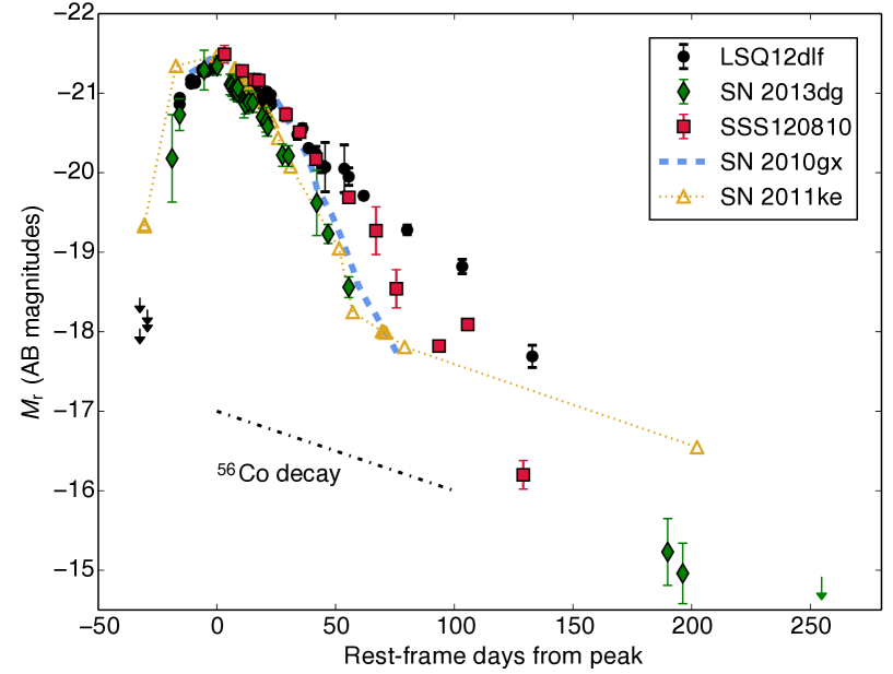
Figure 6: Absolute r-band light curves. Phases have been corrected for time dilation, $K$-corrections (computed using synthetic photometry on our spectra, before and after correcting for cosmological expansion) have been applied to convert the effective filter to rest-frame $r$, and galactic extinction has been accounted for. The rising phases of LSQ12dlf and SN 2013dg are very similar, and last approximately 25–35 days. However, our three objects show quite different declines after maximum light, though all fade more rapidly than fully-trapped ⁵⁶Co decay. Also shown for comparison are SNe 2010gx and 2011ke (typical SLSNe Ic, Inserra et al., 2013).

It is more instructive to directly compare the absolute light curves of our sample. We assume a flat $\Lambda$CDM cosmology, with H${}_{0}=72\,\mathrm{km}\,\mathrm{s}^{-1}\mathrm{Mpc}^{-1}$, $\Omega_{\Lambda}=0.73$ and $\Omega_{\mathrm{M}}=0.27$. Time-dilation, galactic extinction corrections and $K$-corrections have all been applied. The final $r$-band light curves are shown in Figure 6, along with two other SLSNe Ic (2010gx and 2011ke, Pastorello et al., 2010; Inserra et al., 2013). SN 2013dg is most similar to the archetypal SLSNe Ic, including a likely flattening to a tail phase, albeit steeper than that seen in SN 2011ke at 50 days. LSQ12dlf rises with the same gradient as SN 2013dg – the two SNe taking somewhere between 25–35 days to reach peak – but declines significantly more slowly. Moreover, LSQ12dlf shows no sign of a break in the light curve slope even out to 130 days after maximum. SSS120810 declines with a slope intermediate between LSQ12dlf and SN 2013dg. No clear radioactive or magnetar tail is seen; instead we see the rebrightening, which peaks at $\sim$ 100 days after maximum light.

4.3 Bolometric light curves

In order to analyse our data using physical models, we have constructed a bolometric light curve for each of our SNe. First we de-reddened and $k$-corrected our photometry. We then integrated the corrected flux in these optical bands, and applied appropriate corrections for the missing ultra-violet and near-infrared data as follows: Initially, we tried applying corrections based on fitting a blackbody to the optical photometry, and integrating the flux between 1700 Å (approximately the blue edge of the Swift UVOT filters) and 25000 Å. We compared the luminosity in the UV, optical and NIR regimes to the SLSNe studied by Inserra et al. (2013), and found that we were likely significantly over-estimating the UV contribution, as is often the case with blackbody fits. In a real SN, UV absorption lines cause the flux to fall well below that of a blackbody at the optical colour temperature (Chomiuk et al., 2011; Lucy, 1987). We therefore chose not to use the simple blackbody fit in the UV, and instead applied a typical percentage UV correction for SLSNe Ic, using Figure 7 of Inserra et al. (2013). That work included both blackbody fits and real UV data, so should be slightly more reliable. The effect of this correction, and a comparison with SN 2011ke, is shown in our Figure 7. We did continue to use a blackbody estimate for the NIR contribution.

Our bolometric light curves are shown in Figure 8, along with SN 2011ke. Peak luminosities are in the range $0.7-1\times 10^{44}\,\rm{erg}\,\rm{s}^{-1}$. As we saw in our single-filter comparison, the SNe have different declines from maximum. Of our three objects, only SN 2013dg shows evidence of a flattening in the decline rate, though not to the extent seen in SN 2011ke. The bolometric light curve of LSQ12dlf has a similar shape to that of another PESSTO SLSN, CSS121015 (Benetti et al., 2014), though it is significantly less luminous. CSS121015 showed evidence of circumstellar interaction, and the data were consistent with such a shocked-shell scenario, but it also exhibited similarities with SLSNe Ic, and its light curve was satisfactorily reproduced by one of our magnetar models. These two SLSNe show similar rise times and linear declines from peak magnitude. SSS120810 declines more rapidly than LSQ12dlf from a similar peak luminosity, though its linear decline is broken by the rebrightening at 100d. No published SLSN matches this behaviour. Possible mechanisms are proposed in section 6.2

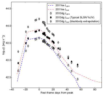
Figure 7: The UV+NIR correction to the $griz$ pseudo-bolometric light curve of SN 2013dg, compared to the bolometric and $griz$ light curves of SN 2011ke (from Inserra et al., 2013). We add the percentage UV flux, as a function of time, for a typical SLSN Ic (Inserra et al., 2013), to SN 2013dg, preserving the similarity in peak luminosity between these two SNe. We model the NIR flux by fitting a blackbody to the optical data. If we do the same for the UV flux, we overestimate the flux contribution from wavelengths shorter than rest-frame $g$-/$B$-band, as shown.

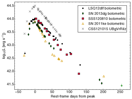
Figure 8: Bolometric light curves of LSQ12dlf, SSS120810, SN 2013dg and SN 2011ke (from Inserra et al., 2013), as well as CSS121015 (a SLSN from PESSTO with spectral similarities to both SLSNe Ic and SLSNe II; Benetti et al., 2014).

5 Light curve models for SLSNe

5.1 Magnetar and radioactive models

In previous works (Inserra et al., 2013; Nicholl et al., 2013; McCrum et al., 2014), we modelled SLSN Ic light curves using a semi-analytic code based on the diffusion solution of Arnett (1982), with radioactive nickel and magnetar radiation as power sources. Our magnetar model takes six parameters, of which the following four are free to vary: the ejected mass ($M_{\rm ej}$), the magnetic field ($B$) and natal spin period ($P$) of the pulsar, and the explosion time ($t_{\rm shift}$). We fix the initial kinetic energy ($E_{\rm k}$) of the ejecta at $10^{51}$erg, and add to this the time-averaged energy input by the magnetar (minus that which is radiated away). The opacity ($\kappa$) is also fixed in our models, at $\kappa=0.2\,{\rm cm}^{2}\,{\rm g}^{-1}$. This choice of value is discussed in section 5.2. The equations determining energy input and output are given in the appendix of Inserra et al. (2013), and are based on the work of Arnett (1982), Ostriker & Gunn (1971) and Kasen & Bildsten (2010). Good agreement has been found with the detailed simulations of Kasen & Bildsten (2010). We fit these models to observed SLSN light curves by $\chi^{2}$ minimisation, after a coarse grid scan through parameter space has initialised the variables with sensible values.

The free parameters in our radioactive decay model are $M_{\rm ej}$, the mass of radioactive ⁵⁶Ni ($M_{\rm Ni}$), $E_{\rm k}$, and $t_{\rm shift}$. We again fix $\kappa$. In this case we omit the formal minimisation of $\chi^{2}$, since this almost invariably returns physically impossible fits, with $M_{\rm Ni}$>$M_{\rm ej}$. Instead we iterate on a finer mass grid (with a resolution of 0.1 M_⊙), for kinetic energies – in units of $10^{51}$erg – of 1, 3, 10 and 30 (if no satisfactory fit is obtained, we also try 100, i.e. in the case of CSS121015).

5.2 Interaction model

The models discussed above showed that the ⁵⁶Ni decay chain struggles to reproduce SLSN Ic light curves, and that magnetar input can power the light curves observed so far. However, they did not allow us to comment quantitatively on the validity of strong interaction with circumstellar material (CSM) as an alternative power source. Mass-loss is a ubiquitous part of stellar evolution, especially in massive stars, and this mass-loss can build up a shell of gas around the star, which the SN ejecta then collide with. Developing a synthetic light curve tool based on ejecta-CSM interaction is therefore an important step in discriminating between the three main models for SLSNe (magnetars, radioactivity and interaction).

We have developed such a code by implementing the formulae detailed in Chatzopoulos, Wheeler & Vinko (2012). Their derivation assumes a stationary photosphere inside the CSM shell – this is justified by the slow expansion velocity of the CSM relative to typical velocities in SNe. Energy is input efficiently by self-similar forward and reverse shocks (i.e. all of the kinetic energy of the shocks converts to radiation) generated at the ejecta-CSM interface (Chevalier, 1982; Chevalier & Fransson, 1994), as well as by radioactive decay of ⁵⁶Ni and ⁵⁶Co deep in the ejecta. In this approximation, the time-dependence of the energy input from the shocks depends only on the density profiles of the interacting media (the ejecta and the CSM). The shock luminosity originates at the ejecta-CSM interface at all times in this model (to make the problem analytically tractable), but two important timescales are found: heat input by the forward shock is terminated abruptly when it breaks out of the CSM, and the reverse shock stops depositing heat when it has swept up all of the ejecta, leading to some discontinuity in the gradient of the light curve at these two epochs.

While the treatment of the shocks is based on that of Chevalier (1982) and Chevalier & Fransson (1994), those works dealt with an optically thin stellar wind, where we normally see X-ray emission from the reverse shock front, and strong narrow lines from pre-shock gas excited by these energetic photons. This is not the case for an optically thick CSM, which is necessary to explain the SLSNe (Smith et al., 2008). In this regime, the diffusion of energy out of the shell is important, and we follow Chatzopoulos, Wheeler & Vinko (2012) in using the formalism of Arnett (1980, 1982), in the special case of zero expansion velocity (our magnetar and nickel models use the same result with homologous expansion). Energy deposited by the shocks diffuses out of the region where the CSM is optically thick, whereas energy from radioactive decays must diffuse out of the combined mass of the ejecta and the optically thick CSM. Thus two different diffusion times are calculated. After shock heating ends, the solution for the light curve is governed simply by radiative diffusion from the opaque shell, unless there is significant heating from radioactivity.

We fit the observed light curves by $\chi^{2}$ minimisation, using mainly the same free parameters as those of Chatzopoulos, Wheeler & Vinko (2012). The output luminosity is a function of ejected mass ($M_{\rm ej}$), CSM mass ($M_{\rm CSM}$), nickel mass ($M_{\rm Ni}$), explosion time ($t_{\rm shift}$), ejecta kinetic energy ($E_{\rm k}$), interaction radius ($R_{0}$), CSM density ($\rho_{\rm CSM}$, as well as density scaling index, $s$), density scaling exponents for the SN core and envelope ($\delta$ and $n$, respectively), and the opacity ($\kappa$). Our code begins by scanning over a grid of points in this high-dimensional parameter space to look for the best approximate solution. This is then the starting point for a more rigorous $\chi^{2}$ minimisation, using the Python module Scipy.Optimize.Fmin.

To reduce the number of free parameters in our fits, we fix several variables at typical values. The most uncertain is perhaps the opacity. For hydrogen-free material, and when electron scattering is the dominant source of opacity, $\kappa$ is often taken to be $0.1\,{\rm cm}^{2}\,{\rm g}^{-1}$ (see Inserra et al., 2013, and references therein). For hydrogen-rich material, $\kappa=0.33\,{\rm cm}^{2}\,{\rm g}^{-1}$ may be more appropriate (Chatzopoulos, Wheeler & Vinko, 2012). Since we do not know the composition of the CSM (but expect it to be H-poor, from the spectra we observe), we take an intermediate value, $\kappa=0.2\,{\rm cm}^{2}\,{\rm g}^{-1}$. For the sake of consistency, we use the same value in our magnetar and radioactive models. In non-interacting models, $\kappa$ enters into the light curve equation only in determining the diffusion timescale parameter: $\tau\propto\kappa^{1/2}M_{\rm ej}^{3/4}E_{\rm k}^{-1/4}$. As $\tau$ is what we really fit for, and $E_{\rm k}$ is either fixed or, in the case of the magnetar, determined from $B$ and $P$, for a given fit we have $M_{\rm ej}$$\,\propto\,\kappa^{-2/3}$. Therefore, varying the opacity by a factor of 2 only changes the extracted mass estimate by a factor $\sim 1.6$, which is not crucial to our analysis.

We fix $n=10$ and $\delta=0$ (Chatzopoulos, Wheeler & Vinko, 2012; Chevalier & Fransson, 1994), and test only $s=0$, corresponding to a uniform density shell produced by a massive outburst of the progenitor, and $s=2$, appropriate for a steady stellar wind prior to explosion. These were the cases studied by Chevalier (1982). There are still many remaining parameters, so Chatzopoulos et al. (2013) were not surprised to find a large degeneracy between them. $M_{\rm ej}$ and $R_{0}$ were particularly weakly constrained, especially if both wind ($s=2$) and shell ($s=0$) models are considered. Because previous interaction-powered models of SLSNe have required very massive CSM, such that the mass loss rates would be extraordinarily high if this material were lost in a steady wind (e.g. see the discussion in Benetti et al., 2014), for this paper we restrict our fits to uniform shells from large mass ejections ($s=0$). We also find that our fits are largely insensitive to the parameter $R_{0}$; it affects the light curve only insofar as it alters the radius of the photosphere ($R_{\rm phot}$). We initially allowed $R_{0}$ to vary from $10^{12}-10^{15}$cm, but the CSM shells we find in fits of SLSNe are all $\sim 10^{15}$cm thick, with the photosphere located close to the outer edge (as expected, since these shells are highly optically thick), so our ‘best-fit’ $R_{0}$ is typically much smaller than $R_{\rm phot}$, and can in fact be changed by factors of 10 or more with little to no effect on the other parameters of the light curve. We therefore fix $R_{0}$ at $10^{13}$cm ($\sim$150 ${\rm R}_{\odot}$) for simplicity. This leaves $M_{\rm ej}$, $M_{\rm CSM}$, $E_{\rm k}$, $\rho_{\rm CSM}$, $t_{\rm shift}$, and (optionally) $M_{\rm Ni}$ as parameters to fit. We have 1–2 more free parameters in this model, compared to the magnetar model, so we expect that it will be easier to fit a wider range of light curve shapes.

The peak luminosity is most sensitive to $E_{\rm k}$ and $M_{\rm ej}$, with more energetic or less massive explosions giving a brighter peak. The light curve timescales depend on $\rho_{\rm CSM}$, $M_{\rm ej}$ and $M_{\rm CSM}$. Denser CSM results in a faster rise but slower decline, whereas more massive CSM tends to broaden the whole light curve, by increasing the diffusion time from the shell. More massive ejecta result in a slower rise, and can broaden the peak as it weakly increases the termination time for the forward shock while greatly increasing that for the reverse shock, but it has little effect on the final decline rate, as the shock energy is input at the base of the CSM shell (however, for significant nickel mass, $M_{\rm ej}$ does affect the diffusion timescale). In most cases, the forward shock luminosity is greater than that of the reverse shock, such that the discontinuity at reverse shock termination is only visible in the light curve if this occurs after forward shock termination.

Of course, there are limitations to this analytical framework, many of which were also pointed out by Chatzopoulos, Wheeler & Vinko (2012). The assumption of 100% efficiency in converting kinetic energy to radiation is unrealistic for models with $M_{\rm CSM}$$<<$$M_{\rm ej}$, and in this case we would also expect the photosphere to expand quickly, since the modest swept-up mass is insufficient to slow it down, in contrast to the fixed photosphere we use in the model. In our fits, we typically find $M_{\rm CSM}$$\sim$$M_{\rm ej}$$/2$, so these approximations are not bad for our purposes. In general, the dynamics of this situation are quite complex; however, comparisons between the analytic models and more realistic hydrodynamics simulations shown in Chatzopoulos, Wheeler & Vinko (2012) show that these simplified models are, at the very least, a useful guide to the regions of parameter space that can generate light curves of interest.

6 Model fits to SLSN data

Table 1: Light curve fit parameters

Magnetar
	$M_{\rm ej}$/M⊙	$B$/$10^{14}$G	$P$/ms	$\chi^{2}/{\rm d.o.f.}$
CSS121015	5.5	2.1	2.0	10.39
LSQ12dlf	10.0	3.7	1.9	5.61
SSS120810	12.5	3.9	1.2	10.63
SN 2013dg	5.4	7.1	2.5	1.01
PTF12dam	9.4	1.2	2.7	0.64
SN 2011ke	6.7	6.4	1.7	1.60
56Ni decay
	$M_{\rm ej}$/M⊙	$M_{\rm Ni}$/M⊙	$E_{\rm k}$/$10^{51}$erg	$\chi^{2}/{\rm d.o.f.}$
CSS121015	20.3	20.2	100	329.14
LSQ12dlf	10.1	8.1	30	3.46
SSS120810	7.2	6.6	30	10.45
SN 2013dg	6.6	5.5	30	0.37
CSM interaction
	$M_{\rm ej}$/M⊙	$M_{\rm CSM}$/M⊙	$M_{\rm Ni}$/M⊙	$E_{\rm k}$/$10^{51}$erg	log($\rho_{\rm CSM}$/${\rm g}\,{\rm cm}^{-3}$)	$\chi^{2}/{\rm d.o.f.}$	$R_{\rm phot}$/$10^{15}$cm (not fit)
CSS121015	6.7	4.9	–	2.3	-12.54	4.12	2.0
LSQ12dlf	7.6	3.4	–	1.1	-11.95	0.80	1.1
SSS120810	15.8	2.3	–	0.84	-11.74	12.78	2.1
SN 2013dg	4.6	2.4	–	1.2	-12.22	0.38	0.6
PTF12dam	26.3	13.0	–	1.9	-12.06	0.45	2.6
SN 2011ke	0.8	0.1	0.3	0.1	-15.07	13.95	2.4
SN 2011ke ($t<50$ d)	10.8	0.1	–	0.07	–9.86	0.26	2.6

In this section we apply our three simple light curve models to the data presented in section 4. We consider magnetar-powered light curves using the same method and analytical treatment discussed and applied by us previously in Inserra et al. (2013), Nicholl et al. (2013) and McCrum et al. (2014). A similar model based on ⁵⁶Ni-powering, as implemented in those same works, is also presented. Those papers showed that magnetar models could reasonably reproduce the bolometric light curves as well as the temperature and velocity evolution. We now also investigate fits with the simple CSM interaction model presented in the previous section. We start by applying these model fits to the three new PESSTO SLSNe, and then put this in context by revisiting three well-studied SLSNe using the CSM alternative model: SN 2011ke (Inserra et al., 2013), PTF12dam (Nicholl et al., 2013) and CSS121015 (Benetti et al., 2014).

The best fitting light curve models for each SN are shown in Figures 9–12, and the parameters of all fits are listed in Table 1. Errors are approximately the same size as the circles. Triangles represent upper limits. In practice, we find that no ⁵⁶Ni is required for the interaction-powered fits to any of our SNe. We have also measured velocities (by fitting Gaussian profiles to spectral lines; errors are the scatter in multiple fits) and temperatures (from the automated blackbody fits to our photometry, used to estimate UV and NIR corrections in section 4.3). These are compared to the predictions of our light curve models. Magnetar and nickel models give us photospheric velocities and temperatures, as described in Inserra et al. (2013); hence these curves end when the SN no longer has a well-defined photosphere (i.e. its atmosphere has become optically thin). The temperature is estimated in our interaction model simply by assuming that the output luminosity is blackbody emission from the photosphere, and therefore using $L=4\pi R_{\rm phot}^{2}\sigma T^{4}$. As the location of the photosphere, $R_{\rm phot}$, is fixed in this model, we simply have $T\propto L^{1/4}$.

6.1 LSQ12dlf

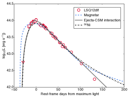
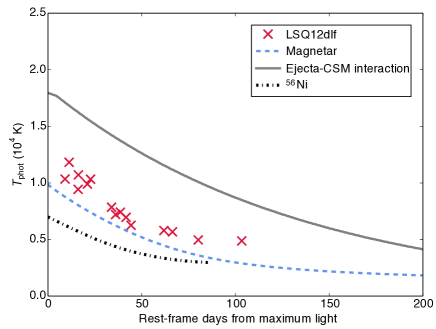
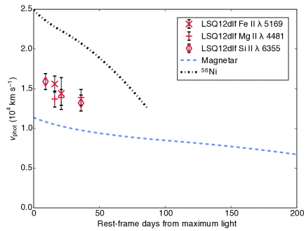
Figure 9: Magnetar-, interaction- and ⁵⁶Ni-powered models of LSQ12dlf. Parameters are listed in Table 1. Temperatures were estimated by fitting blackbody curves to multi-colour photometry; velocities were measured from absorption minima.

In contrast to the SLSNe studied by Inserra et al. (2013), LSQ12dlf (Fig. 9) is difficult to fit with a magnetar model. It has a noticeably broader light curve than all the other low-$z$ SLSNe Ic. The decline in magnitude is linear for $\sim$130 days, showing no sign of a $t^{-2}$ tail (or indeed a ⁵⁶Co tail). Although the magnetar model fits the majority of the light curve well, the fit is poor at late times, where it over-predicts the flux, and early times, as fitting the slow decline results in a broader peak and, more importantly, an earlier explosion date than our limit at -30 days suggests. The peak is not so problematic, since these luminosities are estimated from single-filter LSQ photometry, and are therefore subject to significant uncertainty. The discrepancy between the magnetar model and the data at 130 days could be attributable to time-dependence of the magnetar energy-trapping. Most of the magnetar power is expected to be released in the form of X-rays/$\gamma$-rays and/or high-energy particle pairs; if the ejecta become optically thin to X-rays, for example, as the SN expands, the luminosity emitted as reprocessed optical radiation may drop below the predictions of our fully-trapped model. Therefore we cannot exclude the magnetar based on the late data point.

The interaction and radioactive models give a better fit to the early part of the light curve, though we exclude the latter because of the requirement for 80% nickel ejecta. The interaction model is for $\sim 8$ M_⊙ of ejecta and $\sim 3$ M_⊙ of CSM. This gives a satisfactory fit to the whole light curve.

The magnetar model best matches the temperature evolution, however, all three models get the approximate shape correct. The nickel model greatly over-predicts the SN velocity, because of the large explosion energy ($30\times 10^{51}$erg) needed to fit the light curve time scales. This is true for all of our SNe.

6.2 SSS120810

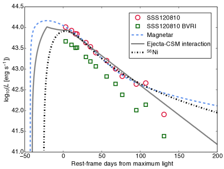
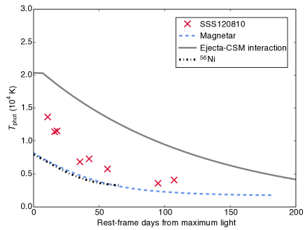
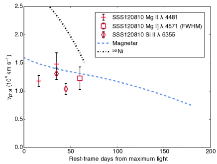
Figure 10: Magnetar-, interaction- and ⁵⁶Ni-powered models of SSS120810. Parameters are listed in Table 1. Temperatures were estimated by fitting blackbody curves to multi-colour photometry; velocities were measured from absorption minima.

This SN is the most difficult to fit, despite the lack of photometry before maximum brightness, because none of our simple light curve models naturally accommodate a late rebrightening as observed in the SSS120810 data. In Figure 10, we show both the bolometric and BVRI pseudo-bolometric light curve, to illustrate the uncertainty in the relative height of this feature. Regardless, the final point on the light curve falls well below the tails of our magnetar and radioactive fits. The interaction fit parameters are quite different from our other light curves, with $M_{\rm ej}$$\sim 16$ M_⊙  and $M_{\rm CSM}$$\sim 2$ M_⊙, whereas the other fits have $M_{\rm ej}$$\sim 4-8$ M_⊙ and $M_{\rm ej}$/$M_{\rm CSM}$$\sim 1.4-2.2$. However, the parameters for SSS120810 are by far the least well-constrained, due to the lack of early data. The magnetar model gives a good fit to the velocity, while the temperature is intermediate between the magnetar and interaction models. We again reject the radioactive model, because of the inferred 90% ⁵⁶Ni ejecta.

One possible explanation for the bump at 100 days could be circumstellar interaction with multiple shells of material. The peak emitted luminosity of a shocked shell should approximately obey the relation (Quimby et al., 2007; Smith & McCray, 2007) $L\sim\frac{1}{2}M_{\rm CSM}v_{\rm phot}^{2}/t_{\rm rise}$, where $v_{\rm phot}$ is the photospheric velocity and $t_{\rm rise}$, the rise time, is a typical light curve timescale. Let us assume that the main light curve peak ($L\sim 10^{44}\,{\rm erg}\,{\rm s}^{-1}$) is powered by an ejecta-CSM interaction as described by our best-fit model in Figure 10 ($M_{\rm ej}$$\sim 16$ M_⊙; $M_{\rm CSM}$$\sim 2$ M_⊙; $t_{\rm rise}\sim 30\,$d). Although our code utilises a simplifying stationary photoshere, in reality the shocked shell is expanding, as momentum must be conserved. If it then encounters further material, another shock, and consequently a rebrightening, may occur, with a luminosity also roughly given by the above expression.

In our case, this anomaly appears to be much faster than the main light curve timescale; the final point on our light curve is consistent with the original decline, suggesting the rebrightening lasts $\la 30\,$d. This in turn suggests a much lower CSM mass compared to the first shell (remembering that $M_{\rm CSM}$ is an important factor in setting the light curve width). In this scenario, we might expect the outer shell to be swept up by the inner shell/ejecta without causing the expanding material to decelerate significantly. Since the shell velocity is then similar before and after the second collision, we may write $(M_{2}/M_{1})\sim(L_{2}/L_{1})(t_{2}/t_{1})$. Fitting a straight line to our bolometric light curve, we find that the bump is $\sim 2.4\times 10^{42}{\rm erg}\,{\rm s}^{-1}$ brighter than the predicted luminosity at this phase, and the rise time is $\ga 10\,$d. This gives an estimated mass of $\ga 0.01$ M_⊙ for the outer CSM. Perhaps this is associated with a normal stellar wind, prior to ejection of the dense shell. There are related alternatives to this picture, for example a single CSM shell, but with clumpy structure in the outer layer. If the forward shock encounters such a clump, the change in density may cause a rebrightening. Another possibility is a change in the density gradient towards the outside of the shell. However, it should be noted that in our fit the forward shock breaks out of the shell around peak, long before the rebrightening.

Another intriguing possibility is that we have the first optical observation of magnetar wind breakout in a SLSN. Metzger & Piro (2014) predict that, under certain conditions, the ionisation front of the pulsar wind nebula could break out of the ejecta a few months after the optical light curve peak. Levan et al. (2013) observed X-ray emission from SCP06F6, one of the first known SLSNe Ic, at just such a phase, but no other SLSNe have been detected in X-rays (limits have been measured by Ofek et al., 2013). Metzger & Piro (2014) found that the ionisation front is more likely to break out (and to break out earlier) for more energetic magnetars, and in fact our fit to SSS120810 suggests a spin period of 1.2 ms – close to the maximum allowed rotation rate for neutron stars. Those authors also point out that X-ray breakout may result in an abrupt change in the optical properties of the SN, such as the effective temperature. Our observations indicate that the rebrightening is more pronounced at bluer wavelengths, and our estimates of the blackbody colour temperature shown in Figure 10 seem to support the idea that the rebrightening is associated with a reheating of the ejecta.

6.3 SN 2013dg

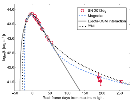
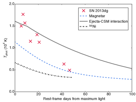
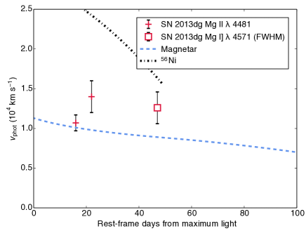
Figure 11: Magnetar-, interaction- and ⁵⁶Ni-powered models of SN 2013dg. Parameters are listed in Table 1. Temperatures were estimated by fitting blackbody curves to multi-colour photometry; velocities were measured from absorption minima.

As shown in section 4, the light curve of SN 2013dg is the most similar to typical low-redshift SLSNe Ic (Inserra et al., 2013). It is well fit by all of our models (Fig. 11), although the composition of our radioactive model is typically unrealistic. Points beyond $\sim 100$ days are required to distinguish between models, as the magnetar light curve predicts a turn-off not seen in the interaction fit. Our observations at $\sim$200d are in line with the magnetar model; however without a template at a phase of $>$1 year, we do not know how much of this flux comes from the host. For this reason, we exclude these points from the interaction fit, which would require substantial ⁵⁶Ni mass to replicate this tail ($\ga 5$ M_⊙, judging from our radioactive fit here). This amount of ⁵⁶Ni would have a significant effect on the light curve peak, and our derived parameters. To investigate this, we apply our code to SN 2011ke, which had a light curve very similar to SN 2013dg up to 50 days (Figures 6 and 8), before slowing in its decline. The results are shown in Figure 12. Fitting the whole 2011ke light curve requires very different parameters to our best-fit model of the peak (and of SN 2013dg) – essentially we require a SN Ia ejecta and nickel mass, embedded in a fairly low-mass CSM, rather than the massive star model fitting the light curve peak (Table 1). We note that similar CSM models have been used to explain super-Chandrasekhar mass SNe Ia (Taubenberger et al., 2011; Scalzo et al., 2014), but that the spectra of such events are very different to SLSNe Ic.

The interaction model does the best job of matching the high early temperatures seen in SN 2013dg, though the SN cools quite quickly, and by 40 days is closer to the magnetar model. The nickel model is rather cool compared to our observations. Measuring the evolution of line velocities proved difficult, as blending meant that few lines were useful at multiple epochs. For example, the maximum of the Fe II feature at $\sim 5200$ Å moves from 5169 Å (the line used for LSQ12dlf) to $\sim 5300$ Å as the spectrum evolves, artificially inflating the measured velocity with time. Nevertheless, the fairly flat velocity curve of our magnetar fit appears to agree with our estimates for the magnesium layer.

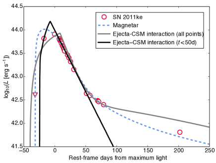
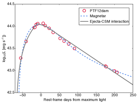
Figure 12: Magnetar- and interaction-powered models of SN 2011ke and PTF12dam. Magnetar fits are the same as those shown in Inserra et al. (2013) and Nicholl et al. (2013). Parameters are listed in Table 1. Top: The light curve of SN 2011ke strongly favours a magnetar. While both models struggle to fit the rise, the magnetar gives a better match to the late tail-phase. In the CSM model, the tail is powered by nickel. The parameters we derive ($M_{\rm ej}$$\sim 0.8$ M_⊙; $M_{\rm Ni}$$\sim 0.3$ M_⊙; $M_{\rm CSM}$$\sim 0.1$ M_⊙) are actually loosely consistent with a SN Ia exploding inside a CSM shell – a ‘Ia-CSM’ (e.g. Silverman et al., 2013; Aldering et al., 2006; Dilday et al., 2012) (but see also Inserra et al., 2014, and references therein). However, its spectrum is that of a typical SLSN Ic, while all existing Ia-CSM candidates have been hydrogen-rich. To fit the first fifty days of the light curve requires no ⁵⁶Ni, but needs $M_{\rm ej}$$\sim 11\,$M_⊙ (and far denser CSM). Bottom: Nicholl et al. (2013) modelled the slowly declining SLSN Ic PTF12dam and, after ruling out ⁵⁶Ni-powered models, suggested a magnetar model. Our expanded fitting routines now show that an interaction fit is also a viable explanation of its unusual light curve. The derived parameters for PTF12dam are actually similar to the majority of our objects, except that the masses of ejecta and CSM are larger by a factor $\sim 5$.

6.4 CSS121015

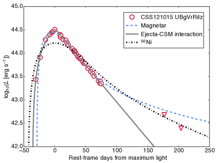
Figure 13: Fits to the pseudo-bolometric light curve of CSS121015 (Benetti et al., 2014), using models powered by magnetar radiation, ejecta-CSM interaction, and ⁵⁶Ni decay. Parameters are listed in Table 1.

The Type II SLSN, CSS121015, was studied by Benetti et al. (2014). They found that the observed properties were broadly consistent with a scenario in which the optical transient is powered by the collision of the SN ejecta with several solar masses of CSM. We fit this SN here (Fig. 13; for parameters see Table 1) – both as an extension of that work, and as a test of our model. Our light curve fit supports the interpretation of those authors, with a best-fit $M_{\rm CSM}$$\sim 5\,$M_⊙, similar to the $\sim 8\,$M_⊙ they estimated. While the quality of fit is similar to that of the magnetar model over the observed lifetime of the SN, the upper limits obtained $\sim$ 200 days after maximum light prove to be useful discriminators. The $t^{-2}$ magnetar tail over-predicts the flux at late epochs, whereas in the interaction model, shock heating terminates a few days after maximum, and the light curve is subsequently just radiative diffusion; the SN therefore lacks a power input to drive a bright tail-phase (though small ⁵⁶Ni mass cannot be excluded, as a radioactive tail similar to normal core-collapse SNe would not have been detected at this distance). This clearly illustrates the utility of our simple models, and lends support to the arguments presented by Benetti et al. (2014). Of course, there is also the possibility that the ejecta no longer traps all of the high-energy magnetar input at late epochs (e.g. Kotera, Phinney & Olinto, 2013), causing the optical emission to drop below the prediction of our fully-trapped model. ⁵⁶Ni cannot be the dominant power source, as our fit is poor even for very optimistic parameters – ejecta composed almost entirely of ⁵⁶Ni, with an explosion energy of $10^{53}$erg.

6.5 CSM configuration

The interaction-powered fits require dense CSM extending to a radius $\sim 10^{15}$cm. To put this in context, we compare the model for LSQ12dlf to the densest known winds from Wolf-Rayet (WR) stars. These have mass-loss rates ($\dot{M}$) approaching $10^{-4}\,$M_⊙ yr^-1, and terminal velocities ($v_{\infty}$) $\sim 1000\,$km s^-1(Crowther, 2007; Gräfener & Hamann, 2008; Hillier & Miller, 1999). This is shown in Figure 14. To find the density profiles generated by these winds, we use the following parameterisation:

$$\dot{M}=4\pi r^{2}\rho(r)v(r),$$ (1)

from the equation of continuity, and

$$v(r)=v_{\infty}(1-R_{*}/r)^{\beta}$$ (2)

(see Crowther, 2007, and references therein), where $R_{*}$ is the stellar radius. We take $R_{*}=20$R_⊙ and $\beta=1$ as fiducial values. Values of $\beta$ between 1–5 are typical, and the inferred density profiles are largely insensitive to these choices.

The WR wind falls orders of magnitude short of the densities in our model fit. To get close to the required density, we need rapid mass loss ($\ga 10^{-2}\,$M_⊙ yr^-1) at fairly low velocity ($v_{\infty}\la 500\,$km s^-1), which probably necessitates a massive outburst shortly before the explosion. As pointed out by Ginzburg & Balberg (2012), the extreme mass-loss needed may help to explain why SLSNe are so rare. Dwarkadas (2007) has simulated how SN evolution occurs in circumstellar environments shaped by Wolf-Rayet stars using mass-loss rates and wind velocities typical of WR stars observed in the Local Group. He finds that the optical and X-ray light curves can be significantly affected, but the mass-loss regime explored ($\dot{M}\sim$ few $\times 10^{-5}\,{\rm M_{\odot}}\,$yr^-1and $v_{\infty}\sim 2000-3000$km s^-1) is much lower than we require for the dense shell scenario.

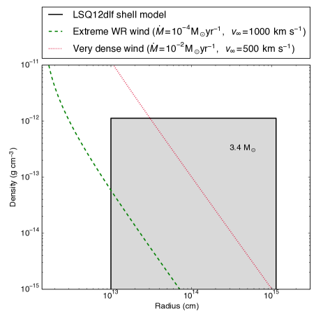
Figure 14: The circumstellar density profile used to fit the light curve of LSQ12dlf with our interaction model. Also shown for comparison are a somewhat extreme Wolf-Rayet wind (green dashed line) and a hypothetical dense, slow wind representing enhanced mass-loss shortly before explosion (red dotted line). This demonstrates the difficulty of achieving very high densities at large radii from the progenitor.

7 Conclusions

We have presented light curves and spectra for the three SLSNe Ic classified in the first year of PESSTO. The spectra appear quite homogeneous, and very much in line with other SLSNe Ic, such as SN 2010gx. Little evolution is seen over the post-maximum photospheric phase, during which time the spectra are dominated by broad lines of singly-ionised metals. Despite this similarity, we see a surprising degree of variety in their light curves, with very different decline rates after maximum and, in the case of SSS120810, evidence of a late re-brightening. SN 2013dg shows a possible break in the decline rate at $\sim 50\,$d, as previously witnessed in SN 2011ke and others. Such a decline break is not seen in SSS120810 or LSQ12dlf. With these very different declines from maximum, we might expect to see these SNe becoming nebular at different relative phases, so coordinating late-time follow-up will be an important step in understanding the nature of these events.

The light curves were analysed using simple diffusion models with radioactivity, magnetar spin-down and ejecta-CSM interaction as power sources. In developing these models, we followed the work of Inserra et al. (2013); Chatzopoulos, Wheeler & Vinko (2012); Arnett (1982); Chevalier & Fransson (1994). We find that none of our light curves can be fit with plausible ⁵⁶Ni-powered models. The typical properties of our interaction fits are: $M_{\rm ej}$$\,\ga 5$ M_⊙; $M_{\rm ej}$/$M_{\rm CSM}$$\sim 1-2$; $E\sim 1-2\times 10^{51}\,$erg; $R_{\rm phot}$$\sim 1-2\times 10^{15}\,$cm; $\log(\rho/{\rm g}\,{\rm cm}^{-2})\sim-12$.

For several objects, the late-time evolution appears to be faint compared to magnetar model predictions. However, our models assume full energy trapping at all epochs, whereas in reality this may be a time-dependent process. Our magnetar tails are thus upper-limits to the late-time luminosities of magnetar-powered SNe.

Inserra et al. (2013) and Nicholl et al. (2013) proposed that magnetar-powered models could explain all of the SLSNe Ic then known, whereas other authors, such as Chatzopoulos et al. (2013) and Benetti et al. (2014), favour circumstellar interaction. Our fits here reinforce the validity of both of these interpretations, without particularly favouring either. More detailed hydrodynamical light curve modelling and synthetic spectra are needed to disentangle the signatures of these two possible power sources. In particular, it remains to be seen whether interaction models can reproduce the observed spectra, and if so, under what conditions. If there are two mechanisms at play, we need to understand how these very different processes produce such similar spectra. No SLSN Ic to date has shown narrow lines, the traditional signature of circumstellar interaction (though some SLSNe II, such as CSS121015, showed narrow H lines as well as marked similarity to SLSNe Ic), so the next step is to investigate whether we should expect this to be the case for the regimes of density, temperature and opacity needed to reproduce the light curves (and how this differs from Type Ic SN 2010mb, a lower luminosity pulsational-PISN candidate that did show narrow oxygen lines; Ben-Ami et al., 2014). Additionally, the presence of broad SN lines in the early spectra may be inconsistent with the presence of an obscuring circumstellar shell. On the observational side, probing the physics of SLSNe will require spectra at very late times, to examine the ejecta composition, and more data in the high-energy regime, to look for signatures of magnetar wind breakout.

ACKNOWLEDGMENTS This work is based on observations collected at the European Organisation for Astronomical Research in the Southern Hemisphere, Chile as part of PESSTO (the Public ESO Spectroscopic Survey for Transient Objects), ESO program ID 188.D-3003. VLT+X-shooter spectra were obtained under ESO programs 089.D-0270 and 091.D-0749. Other observations have been collected using: the 4.3m William Herschel Telescope, operated on the island of La Palma by the Isaac Newton Group of Telescope; the Liverpool Telescope, which is operated by Liverpool John Moores University in the Spanish Observatorio del Roque de los Muchachos of the Instituto de Astrofisica de Canarias with financial support from the UK Science and Technology Facilities Council; the Las Cumbres Observatory Global Telescope Network (LCOGTN); the Gemini Observatory, which is operated by the Association of Universities for Research in Astronomy, Inc., under a cooperative agreement with the NSF on behalf of the Gemini partnership: the National Science Foundation (United States), the National Research Council (Canada), CONICYT (Chile), the Australian Research Council (Australia), Ministério da Ciência, Tecnologia e Inovação (Brazil) and Ministerio de Ciencia, Tecnología e Innovación Productiva (Argentina). Research leading to these results has received funding from the European Research Council under the European Union’s Seventh Framework Programme (FP7/2007-2013)/ERC Grant agreement n^o [291222] (PI S.J.S). We acknowledge funding from STFC and DEL NI. S.B. is partially supported by the PRIN-INAF 2011 with the project Transient Universe: from ESO Large to PESSTO . M.F. was partly supported by the European Union FP7 programme through ERC grant number 320360. N.E.R. acknowledges the support from the European Union Seventh Framework Programme (FP7/2007-2013) under grant agreement n. 267251 “Astronomy Fellowships in Italy” (AstroFIt). A.G.-Y. is supported by “The Quantum Universe I-Core program by the Israeli Committee for planning and funding and the ISF, a GIF grant, and the Kimmel award.

Table 2: Spectroscopic observations of LSQ12dlf

date	MJD	phase*	Setup	range (Å)	Resolution (Å)
2012-08-07	56147.3	+7	NTT+EFOSC2	3700-9200	18
2012-08-09	56149.3	+9	NTT+EFOSC2	3400-10000	13
2012-08-18	56158.3	+16	NTT+EFOSC2	3700-9200	18
2012-08-24	56164.3	+21	NTT+EFOSC2	3700-9200	18
2012-09-09	56180.3	+34	NTT+EFOSC2	3700-9200	18
2012-09-12	56182.5	+36	VLT+Xshooter	3100-24000	1
2012-09-22	56193.3	+44	NTT+EFOSC2	3700-9200	18
2012-12-09	56270.5	+106	Gemini S.+GMOS	4660-8900	2

* Phase in rest-frame days relative to epoch of maximum light.

Table 3: Spectroscopic observations of SSS120810

date	MJD	phase*	Setup	range (Å)	Resolution (Å)
2012-08-17	56158.3	+10	NTT+EFOSC2	3700–9200	18
2012-08-18	56158.3	+11	NTT+EFOSC2	3700–9200	18
2012-08-24	56164.3	+16	NTT+EFOSC2	3700–9200	18
2012-09-15	56186.2	+35	NTT+EFOSC2	3700–9200	18
2012-09-23	56194.2	+42	NTT+EFOSC2	3700–9200	18
2012-09-26	56196.5	+44	VLT+Xshooter	3100–24000	1
2012-10-14	56215.3	+60	NTT+EFOSC2	3700–9200	18

* Phase in rest-frame days relative to epoch of maximum light.

Table 4: Spectroscopic observations of SN 2013dg

date	MJD	phase*	Setup	range (Å)	Resolution (Å)
2013-06-10	56454.0	+4	WHT+ISIS	3260–10000	$4.1-7.7$
2013-06-13	56457.0	+6	Gemini S.+GMOS	4660–8900	2
2013-06-25	56469.0	+16	VLT+Xshooter	3100–24000	1
2013-07-03	56477.0	+22	Gemini S.+GMOS	4660–8900	2
2013-07-20	56493.0	+35	VLT+Xshooter	3100–24000	1
2012-08-03	56508.0	+47	Gemini S.+GMOS	4660–8900	2

* Phase in rest-frame days relative to epoch of maximum light.

Table 5: Observed photometry of LSQ12dlf

Date	MJD	Phase∗	U	B	V	R	I	Instrument∗∗
2012-06-18	56097.41	-32.7			>22.32			LSQ
2012-06-18	56097.44	-32.6			>21.93			LSQ
2012-06-22	56101.36	-29.5			>22.08			LSQ
2012-06-22	56101.41	-29.5			>22.17			LSQ
2012-07-09	56118.35	-15.9			19.33 (0.03)			LSQ
2012-07-09	56118.41	-15.9			19.25 (0.02)			LSQ
2012-07-15	56124.41	-11.1			19.07 (0.02)			LSQ
2012-07-15	56124.43	-11.1			19.02 (0.02)			LSQ
2012-07-17	56126.41	-9.5			19.04 (0.03)			LSQ
2012-07-17	56126.43	-9.5			19.06 (0.03)			LSQ
2012-07-21	56130.31	-6.4			18.89 (0.03)			LSQ
2012-07-21	56130.38	-6.3			18.92 (0.03)			LSQ
2012-07-23	56132.41	-4.7			18.92 (0.02)			LSQ
2012-07-23	56132.42	-4.7			18.91 (0.02)			LSQ
2012-07-27	56136.24	-1.6			18.87 (0.04)			LSQ
2012-07-27	56136.32	-1.5			18.90 (0.02)			LSQ
2012-07-29	56138.25	0.0			18.78 (0.04)			LSQ
2012-07-29	56138.34	0.1			18.80 (0.03)			LSQ
2012-08-09	56149.40	8.9	18.46 (0.09)	19.43 (0.04)	19.15 (0.04)	19.01 (0.09)	18.82 (0.10)	NTT
2012-08-12	56152.10	11.1		19.45 (0.23)	19.22 (0.14)	19.09 (0.15)	18.93 (0.12)	LT
2012-08-18	56158.10	15.9		19.71 (0.13)	19.22 (0.10)	18.96 (0.06)	18.91 (0.05)	LT
2012-08-18	56158.30	16.0	18.91 (0.09)	19.63 (0.06)	19.26 (0.07)	19.04 (0.05)	18.83 (0.17)	NTT
2012-08-18	56158.40	16.1			19.29 (0.02)			LSQ
2012-08-18	56158.41	16.1			19.39 (0.03)			LSQ
2012-08-20	56160.31	17.6			19.39 (0.08)			LSQ
2012-08-20	56160.39	17.7			19.44 (0.03)			LSQ
2012-08-24	56164.30	20.8	19.34 (0.07)	19.90 (0.04)	19.42 (0.03)	19.20 (0.04)	18.88 (0.05)	NTT
2012-08-24	56164.35	20.9			19.49 (0.03)			LSQ
2012-08-24	56164.38	20.9			19.60 (0.04)			LSQ
2012-08-26	56166.21	22.4			19.53 (0.04)			LSQ
2012-08-26	56166.29	22.4			19.45 (0.03)			LSQ
2012-08-26	56166.40	22.5	19.48 (0.03)	19.99 (0.03)	19.59 (0.04)	19.27 (0.04)	19.00 (0.04)	NTT
2012-09-09	56180.40	33.7	20.31 (0.34)	20.69 (0.08)	20.07 (0.06)	19.59 (0.06)	19.13 (0.09)	NTT
2012-09-12	56183.10	35.9		20.86 (0.15)	20.00 (0.05)	19.50 (0.07)	19.43 (0.10)	LT
2012-09-15	56186.30	38.4		21.05 (0.03)	20.24 (0.02)	19.79 (0.03)	19.45 (0.04)	NTT
2012-09-19	56190.10	41.5		21.28 (0.18)	20.30 (0.09)	19.82 (0.06)	19.57 (0.13)	LT
2012-09-22	56193.40	44.1		21.62 (0.07)	20.46 (0.07)	19.92 (0.06)	19.56 (0.05)	NTT
2012-09-24	56195.00	45.4			20.49 (0.31)	19.98 (0.16)	19.64 (0.16)	LT
2012-10-04	56205.10	53.5			20.66 (0.30)	20.12 (0.10)	20.01 (0.13)	LT
2012-10-06	56207.40	55.3			20.79 (0.11)	20.11 (0.15)	19.63 (0.24)	NTT
2012-10-12	56213.00	59.8			21.20 (0.20)	20.44 (0.20)	20.01 (0.18)	LT
2012-10-20	56221.00	66.2		22.64 (0.31)	21.16 (0.19)	20.76 (0.18)	20.45 (0.14)	LT
2012-11-06	56238.20	80.0		23.32 (0.07)	21.92 (0.06)	21.18 (0.05)	20.59 (0.04)	NTT
2012-12-05	56267.20	103.2		24.43 (0.33)	22.82 (0.09)	22.17 (0.08)	21.72 (0.51)	NTT
2012-01-04	56297.00	127.2				22.71 (0.30)		NTT
2012-01-11	56304.10	132.7			24.00 (0.14)			NTT
2013-10-09 (host)	56575.3	354.8			25.02 (0.15)	$>23.98$	$>22.65$	NTT
2014 stack (host)$\ddagger$					24.81 (0.34)			NTT

* Phase in rest-frame days from epoch of maximum light

** LSQ = La Silla QUEST survey

NTT = ESO NTT + EFOSC2 (PESSTO)

LT = Liverpool Telescope + RATCam

$\ddagger$ Sum of images obtained on 4 nights in Jan and Feb 2014

Table 6: Observed photometry of SSS120810

Date	MJD	Phase∗	U	B	V	R	I	Instrument∗∗
2012-08-10	56149.7	3.2				17.76 (0.11)		SSS
2012-08-18	56158.3	10.6	17.38 (0.03)	18.16 (0.03)	18.09 (0.02)	17.97 (0.02)	17.82 (0.03)	NTT
2012-08-24	56164.3	15.8	17.68 (0.01)	18.42 (0.01)	18.23 (0.02)	18.11 (0.02)	17.90 (0.03)	NTT
2012-08-26	56166.4	17.6	17.80 (0.01)	18.44 (0.02)	18.22 (0.02)	18.12 (0.02)	17.93 (0.02)	NTT
2012-09-08	56179.6	29.1				18.57 (0.09)		SSS
2012-09-15	56186.3	34.9	19.92 (0.03)	19.99 (0.01)	19.21 (0.02)	18.80 (0.02)	18.42 (0.02)	NTT
2012-09-23	56194.3	41.8	20.63 (0.12)	20.56 (0.03)	19.62 (0.02)	19.14 (0.03)	18.70 (0.04)	NTT
2012-10-09	56210.3	55.6		21.26 (0.14)	20.27 (0.06)	19.69 (0.06)	19.14 (0.17)	NTT
2012-10-23	56223.5	67.0			20.78 (0.30)	20.12 (0.30)	19.58 (0.30)	FTS
2012-11-02	56233.4	75.6				20.85 (0.24)		FTS
2012-11-22$\ddagger$	56254.2	93.6		24.62 (0.50)	23.16 (0.13)	21.57 (0.07)	20.88 (0.07)	NTT
2012-12-06$\ddagger$	56268.2	105.7		24.20 (0.38)	22.33 (0.08)	21.30 (0.07)	20.72 (0.10)	NTT
2013-01-02$\ddagger$	56295.2	129.0		$>25.39$	$>25.06$	23.19 (0.18)		NTT
2013-10-09 (host)	56575.1	371.2				21.89 (0.07)	21.14 (0.07)	NTT
2013-10-24 (host)	56590.0	384.1		22.91 (0.06)	22.27 (0.04)			NTT

* Phase in rest-frame days from estimated epoch of maximum light

** SSS = Siding Springs Survey (CRTS)

NTT = ESO NTT + EFOSC2 (PESSTO)

FTS = Faulkes Telescope South + Faulkes Spectral 01

$\ddagger$ Magnitudes measured after subtracting host images from Oct 2013

Table 7: Observed photometry of SN 2013dg

Date	MJD	Phase∗	$g$	$r$	$i$	$z$	Instrument∗∗
2013-05-13	56425.2	-19.0		20.27 (0.54)			CSS
2013-05-17	56429.2	-15.9		19.72 (0.17)			MLS
2013-05-30	56442.2	-5.6		19.16 (0.23)			CSS
2013-06-06	56449.2	0.0		19.11 (0.17)			CSS
2013-06-12	56456.0	5.4	19.26 (0.03)	19.31 (0.06)	19.50 (0.07)	19.60 (0.07)	LT
2013-06-13	56456.9	6.1	19.36 (0.03)	19.31 (0.06)	19.56 (0.10)		LCO
2013-06-14	56457.9	6.9	19.26 (0.07)	19.36 (0.04)	19.39 (0.08)	19.40 (0.17)	LT
2013-06-15	56459.1	7.9	19.41 (0.03)	19.36 (0.07)			LCO
2013-06-15	56459.3	8.0			19.47 (0.08)	19.44 (0.22)	FTN
2013-06-16	56459.9	8.5	19.42 (0.10)	19.39 (0.05)	19.56 (0.10)	19.69 (0.15)	LT
2013-06-16	56460.1	8.7	19.48 (0.06)	19.34 (0.05)			LCO
2013-06-19	56463.4	11.3		19.52 (0.17)			FTN
2013-06-20	56464.1	11.8	19.57 (0.05)	19.55 (0.05)	19.68 (0.12)		LCO
2013-06-22	56465.9	13.3	19.68 (0.10)	19.52 (0.09)	19.71 (0.13)	19.62 (0.20)	LT
2013-06-25	56468.0	14.9	19.81 (0.05)	19.54 (0.05)	19.61 (0.05)		LCO
2013-06-29	56473.0	18.9	20.03 (0.03)	19.74 (0.03)	20.04 (0.22)	19.74 (0.19)	LT
2013-07-01	56475.0	20.5	20.20 (0.03)	19.81 (0.04)	19.93 (0.06)		LCO
2013-07-01	56475.3	20.7	20.25 (0.17)	19.80 (0.14)	19.84 (0.08)	19.92 (0.18)	FTN
2013-07-02	56476.0	21.3	20.26 (0.04)	19.87 (0.04)	20.02 (0.08)		LCO
2013-07-10	56483.8	27.5	20.71 (0.08)	20.23 (0.08)	20.27 (0.11)		LCO
2013-07-13	56487.0	30.0	20.95 (0.07)	20.23 (0.06)	20.24 (0.11)		FTN
2013-07-29	56502.0	41.9	21.48 (0.23)	20.82 (0.39)	20.88 (0.22)	20.52 (0.30)	NTT
2013-08-03	56508.0	46.7	22.23 (0.05)	21.21 (0.04)	20.95 (0.06)	20.79 (0.10)	NTT
2013-08-14	56519.0	55.4		21.88 (0.07)			NTT
2013-08-15	56520.0	56.2			21.62 (0.16)		NTT
2013-08-16	56520.5	56.6				20.91 (0.30)	NTT
2014-01-30$\ddagger$	56688.3	189.8		25.21 (0.41)	24.68 (0.28)		NTT
2014-02-07$\ddagger$	56696.3	196.1		25.48 (0.36)	25.21 (0.36)		NTT
2014-04-22	56770.0	254.6		$>25.63$	$>25.06$		NTT

* Phase in rest-frame days from epoch of maximum light

** CSS = Catalina Sky Survey Survey (CRTS)

MLS = Mt. Lemmon Survey (CRTS)

LT = Liverpool Telescope + RATCam

LCO = Las Cumbres Observatory Global Telesope 1m Network

FTN = Faulkes Telescope North + Faulkes Spectral 02

NTT = ESO NTT + EFOSC2 (PESSTO)

$\ddagger$ May include significant host contribution

References

- Alard & Lupton (1998) Alard C., Lupton R. H., 1998, The Astrophysical Journal, 503, 325
- Aldering et al. (2006) Aldering G. et al., 2006, The Astrophysical Journal, 650, 510
- Arnett (1980) Arnett W. D., 1980, The Astrophysical Journal, 237, 541
- Arnett (1982) Arnett W. D., 1982, The Astrophysical Journal, 253, 785
- Baltay et al. (2013) Baltay C. et al., 2013, Publications of the Astronomical Society of the Pacific, 125, 683
- Barbary et al. (2009) Barbary K. et al., 2009, The Astrophysical Journal, 690, 1358
- Barkat, Rakavy & Sack (1967) Barkat Z., Rakavy G., Sack N., 1967, Physical Review Letters, 18, 379
- Ben-Ami et al. (2014) Ben-Ami S. et al., 2014, The Astrophysical Journal, 785, 37
- Benetti et al. (2014) Benetti S. et al., 2014, Monthly Notices of the Royal Astronomical Society, accepted
- Brown et al. (2013) Brown T. et al., 2013, Publications of the Astronomical Society of the Pacific, 125, 1031
- Buzzoni et al. (1984) Buzzoni B. et al., 1984, The Messenger, 38, 9
- Chatzopoulos, Wheeler & Vinko (2012) Chatzopoulos E., Wheeler J. C., Vinko J., 2012, The Astrophysical Journal, 746, 121
- Chatzopoulos et al. (2013) Chatzopoulos E., Wheeler J. C., Vinko J., Horvath Z., Nagy A., 2013, The Astrophysical Journal, 773, 76
- Chen et al. (2013) Chen T.-W. et al., 2013, The Astrophysical Journal, 763, L28
- Chevalier (1982) Chevalier R. A., 1982, The Astrophysical Journal, 258, 790
- Chevalier & Fransson (1994) Chevalier R. A., Fransson C., 1994, The Astrophysical Journal, 420, 268
- Chevalier & Irwin (2011) Chevalier R. A., Irwin C. M., 2011, The Astrophysical Journal Letters, 729, L6
- Chomiuk et al. (2011) Chomiuk L. et al., 2011, The Astrophysical Journal, 743, 114
- Cooke et al. (2012) Cooke J. et al., 2012, Nature, 491, 228
- Crowther (2007) Crowther P. A., 2007, Annual Review of Astronomy and Astrophysics, 45, 177
- Dessart et al. (2012) Dessart L., Hillier D. J., Waldman R., Livne E., Blondin S., 2012, Monthly Notices of the Royal Astronomical Society: Letters, 426, L76
- Dexter & Kasen (2013) Dexter J., Kasen D., 2013, The Astrophysical Journal, 772, 30
- Dilday et al. (2012) Dilday B. et al., 2012, Science, 337, 942
- Drake et al. (2009) Drake A. et al., 2009, The Astrophysical Journal, 696, 870
- Dwarkadas (2007) Dwarkadas V. V., 2007, The Astrophysical Journal, 667, 226
- Gal-Yam (2012) Gal-Yam A., 2012, Science, 337, 927
- Gal-Yam et al. (2009) Gal-Yam A. et al., 2009, Nature, 462, 624
- Ginzburg & Balberg (2012) Ginzburg S., Balberg S., 2012, The Astrophysical Journal, 757, 178
- Gräfener & Hamann (2008) Gräfener G., Hamann W.-R., 2008, Astronomy and Astrophysics, 482, 945
- Hillier & Miller (1999) Hillier D. J., Miller D., 1999, The Astrophysical Journal, 519, 354
- Hook et al. (2004) Hook I., Jørgensen I., Allington-Smith J., Davies R., Metcalfe N., Murowinski R., Crampton D., 2004, Publications of the Astronomical Society of the Pacific, 116, 425
- Howell et al. (2013) Howell D. et al., 2013, The Astrophysical Journal, 779, 98
- Inserra et al. (2013) Inserra C. et al., 2013, The Astrophysical Journal, 770, 128
- Inserra et al. (2014) Inserra C. et al., 2014, Monthly Notices of the Royal Astronomical Society: Letters, 437, L51
- Inserra et al. (2012) Inserra C. et al., 2012, The Astronomer’s Telegram, 4329, 1
- Kaiser et al. (2010) Kaiser N. et al., 2010, in SPIE Astronomical Telescopes+ Instrumentation, International Society for Optics and Photonics, pp. 77330E–77330E
- Kasen & Bildsten (2010) Kasen D., Bildsten L., 2010, The Astrophysical Journal, 717, 245
- Kotera, Phinney & Olinto (2013) Kotera K., Phinney E. S., Olinto A. V., 2013, Monthly Notices of the Royal Astronomical Society, 432, 3228
- Levan et al. (2013) Levan A. J., Read A., Metzger B., Wheatley P., Tanvir N., 2013, The Astrophysical Journal, 771, 136
- Lucy (1987) Lucy L., 1987, Astronomy and Astrophysics, 182, L31
- McCrum et al. (2014) McCrum M. et al., 2014, Monthly Notices of the Royal Astronomical Society, 437, 656
- Metzger & Piro (2014) Metzger B. D., Piro A. L., 2014, Monthly Notices of the Royal Astronomical Society, 439, 3916
- Miller et al. (2009) Miller A. et al., 2009, The Astrophysical Journal, 690, 1303
- Nicholl et al. (2013) Nicholl M. et al., 2013, Nature, 502, 346
- Ofek et al. (2007) Ofek E. et al., 2007, The Astrophysical Journal Letters, 659, L13
- Ofek et al. (2013) Ofek E. O. et al., 2013, The Astrophysical Journal, 763, 42
- Ostriker & Gunn (1971) Ostriker J. P., Gunn J. E., 1971, The Astrophysical Journal, 164, L95
- Pastorello et al. (2010) Pastorello A. et al., 2010, The Astrophysical Journal Letters, 724, L16
- Quimby et al. (2007) Quimby R. M., Aldering G., Wheeler J. C., Höflich P., Akerlof C. W., Rykoff E. S., 2007, The Astrophysical Journal Letters, 668, L99
- Quimby et al. (2011) Quimby R. M. et al., 2011, Nature, 474, 487
- Rakavy & Shaviv (1967) Rakavy G., Shaviv G., 1967, The Astrophysical Journal, 148, 803
- Rau et al. (2009) Rau A. et al., 2009, Publications of the Astronomical Society of the Pacific, 121, 1334
- Scalzo et al. (2014) Scalzo R. et al., 2014, arXiv preprint arXiv:1404.1002
- Schlafly & Finkbeiner (2011) Schlafly E. F., Finkbeiner D. P., 2011, The Astrophysical Journal, 737, 103
- Silverman et al. (2013) Silverman J. M. et al., 2013, The Astrophysical Journal Supplement Series, 207, 3
- Smartt et al. (2013) Smartt S. J., Nicholl M., Inserra C., Wright D., Chen T.-W., Lawrence A., Mead A., 2013, The Astronomer’s Telegram, 5128, 1
- Smartt et al. (2014) Smartt S. J. et al., 2014, The Messenger, 154, 50
- Smith et al. (2008) Smith N., Chornock R., Li W., Ganeshalingam M., Silverman J. M., Foley R. J., Filippenko A. V., Barth A. J., 2008, The Astrophysical Journal, 686, 467
- Smith et al. (2007) Smith N. et al., 2007, The Astrophysical Journal, 666, 1116
- Smith & McCray (2007) Smith N., McCray R., 2007, The Astrophysical Journal Letters, 671, L17
- Steele et al. (2004) Steele I. A. et al., 2004, Astronomical Telescopes and Instrumentation, 679
- Taubenberger et al. (2011) Taubenberger S. et al., 2011, Monthly Notices of the Royal Astronomical Society, 412, 2735
- Thomas, Nugent & Meza (2011) Thomas R., Nugent P., Meza J., 2011, Publications of the Astronomical Society of the Pacific, 123, 237
- Van Dokkum (2001) Van Dokkum P. G., 2001, Publications of the Astronomical Society of the Pacific, 113, 1420
- Vernet et al. (2011) Vernet J. et al., 2011, Astronomy & Astrophysics, 536, 105
- Woosley (2010) Woosley S., 2010, The Astrophysical Journal Letters, 719, L204
- Woosley, Blinnikov & Heger (2007) Woosley S., Blinnikov S., Heger A., 2007, Nature, 450, 390
- Yaron & Gal-Yam (2012) Yaron O., Gal-Yam A., 2012, Wiserep — an interactive supernova data repository
- Young et al. (2010) Young D. et al., 2010, Astronomy and Astrophysics, 512