Electrocaloric effect in KH₂PO₄

Abstract

The proton ordering model for the KH₂PO₄ type ferroelectrics is modified by taking into account non-linear effects, namely, the dependence of the effective dipole moments on the proton ordering parameter. Within the four-particle cluster approximation we calculate the crystal polarization, longitudinal dielectric permittivity, specific heat, and explore the electrocaloric effect. Smearing of the ferroelectric phase transition by the longitudinal electric field is described. A good agreement with experiment is obtained.

Key words: electrocaloric effect, KDP, cluster approximation, polarization

PACS numbers: 77.84.Fa, 77.70.+a

1 Introduction

At the moment, the largest electrocaloric (EC) effect, which is the change of temperature of a dielectric at an adiabatic change of the applied electric field, is observed in perovskite ferroelectrics. Thus, in [1] in the PbZr_0.95Ti_0.05O₃ thin film with a thickness of 350 nm in a strong electric field (480 kV/cm) the obtained electrocaloric temperature change is $\Delta T=12$ K. Ab initio molecular dynamics calculations [2] predict $\Delta T\thickapprox 20$ K in LiNbO₃. In cheaper and more readily available hydrogen bonded ferroelectrics of the KH₂PO₄ (KDP) type the electrocaloric effect was studied for relatively low fields only. Thus, it has been obtained that $\Delta T\thickapprox 0.04$ K at $E\thickapprox 4$ kV/cm [3], $\Delta T\thickapprox~{}1$ K at $E\thickapprox 12$ kV/cm [4], and $\Delta T\thickapprox 0.25$ K at $T_{c}$ and $E\thickapprox 1.2$ kV/cm [5]. The electrocaloric effect in KDP in high fields remains unexplored.

Theoretically the electrocaloric effect in KDP has been described in [6] within the Slater model [7] and in the paraelectric phase only. However, the Slater model is known to give incorrect results in the ferroelectric phase. Influence of electric field on the thermodynamic characteristics of the KDP type crystals, such as polarization, dielectric permittivity, piezoelectric coefficients, elastic constants has been described in [8, 9, 11] within the proton ordering model with the piezoelectric coupling to the shear strain $\varepsilon_{6}$ and proton tunneling [10] taken into account. However, these theories required, in particular, invoking two different values of the effective dipole moments for the paraelectric and ferroelectric phase [8, 11]. This made a correct description of the system behavior in the fields high enough to smear out the first order phase transition impossible.

In the present paper we suggest a way to circumvent this difficulty. Assuming that the difference between the dipole moments is caused by non-zero values of the order parameter, we modify the proton ordering model accordingly. The crystal characteristics in zero field and in high fields are calculated. Smearing of the first order phase transition and the electrocaloric effect are described.

2 Thermodynamic characteristics

We consider the KDP type ferroelectrics in presence of the external shear stress $\sigma_{6}=\sigma_{xy}$ and electric field $E_{3}$ applied along the crystallographic axis c, inducing the strain $\varepsilon_{6}$ and polarization $P_{3}$. The total model Hamiltonian reads [9]

$$\hat{H}=N\hat{H}_{0}+\hat{H}_{s},$$ (1)

where $N$ is the total number of primitive cells; The “seed” energy corresponds to the sublattice of heavy ions and does not depend explicitly on the deuteron subsystem configuration. It is expressed in terms of the strain $\varepsilon_{6}$ and electric field $E_{3}$ and includes the elastic, piezoelectric, and dielectric contributions

$$\hat{H}_{0}={v}\left(\frac{1}{2}c_{66}^{E0}\varepsilon_{6}^{2}-e_{36}^{0}E_{3}\varepsilon_{6}-\frac{1}{2}\chi_{33}^{\varepsilon 0}E_{3}^{2}\right),$$ (2)

where $v$ is the primitive cell volume; $c_{44}^{E0}$, $e_{36}^{0}$, ${\chi}_{33}^{\varepsilon 0}$ are the “seed” elastic constant, piezoelectric coefficient, and dielectric susceptibility.

The pseudospin part of the Hamiltonian reads

$$\!\!\!\!\!\!\!\!\!\!\!\!\!\!\!\!\hat{H}_{s}=\frac{1}{2}\sum\limits_{{qf}\atop{q^{\prime}f^{\prime}}}J_{ff^{\prime}}(qq^{\prime})\frac{\sigma_{qf}}{2}\frac{\sigma_{q^{\prime}f^{\prime}}}{2}+\hat{H}_{sh}+\sum\limits_{qf}2\psi_{6}\varepsilon_{6}\frac{\sigma_{qf}}{2}-\sum\limits_{qf}\mu_{f}E_{3}\frac{\sigma_{qf}}{2}+\hat{H}_{E}.$$ (3)

Here the first term describes the effective long-range interactions between protons, including also indirect lattice-mediated interactions [12, 13], $\sigma_{qf}$ is the operator of the $z$-component of a pseudospin, corresponding to the proton on the $f$-th hydrogen bond ($f$=1,2,3,4) in the $q$-th cell. Its eigenvalues $\sigma_{qf}=\pm 1$ are assigned to two equilibrium positions of a proton on this bond

In (3) $\hat{H}_{sh}$ is the Hamiltonian of the short-range interactions between protons, which includes linear over the strain $\varepsilon_{6}$ terms [9, 11]

$$\hat{H}_{sh}=\sum\limits_{q}\Bigl{\{}\left(\frac{\delta_{s}}{8}\varepsilon_{6}+\frac{\delta_{1}}{4}\varepsilon_{6}\right)(\sigma_{q1}+\sigma_{q2}+\sigma_{q3}+\sigma_{q4})+$$

$$+\!\left(\frac{\delta_{s}}{8}\varepsilon_{6}-\frac{\delta_{1}}{4}\varepsilon_{6}\right)(\sigma_{q1}\sigma_{q2}\sigma_{q3}\!+\!\sigma_{q1}\sigma_{q2}\sigma_{q4}\!+\!\sigma_{q1}\sigma_{q3}\sigma_{q4}\!+\!\sigma_{q2}\sigma_{q3}\sigma_{q4})+$$

$$+\frac{1}{4}(V+\delta_{a}\varepsilon_{6})(\sigma_{q1}\sigma_{q2}+\sigma_{q3}\sigma_{q4})+\frac{1}{4}(V-\delta_{a}\varepsilon_{6})(\sigma_{q2}\sigma_{q3}+\sigma_{q4}\sigma_{q1})+$$ (4)

$$+\!\frac{1}{4}U(\sigma_{q1}\sigma_{q3}\!+\!\sigma_{q2}\sigma_{q4})\!+\!\frac{1}{16}\Phi\sigma_{q1}\sigma_{q2}\sigma_{q3}\sigma_{q4}\Bigr{\}}.$$

Here

$$V=-\frac{1}{2}w_{1},~{}~{}U=\frac{1}{2}w_{1}-\varepsilon,~{}~{}\Phi=4\varepsilon-8w+2w_{1},$$

where $\varepsilon$ $w$, $w_{1}$ are the energies of proton configurations.

The third term in (3) is a linear over the shear strain $\varepsilon_{6}$ field due to the piezoelectric coupling; $\psi_{6}$ is the deformational potential [9].

The fourth term in (3) effectively describes the system interaction with the external electric field $E_{3}$. Here $\mu_{f}$ is the effective dipole moment of the $f$-the hydrogen bond, and

$$\mu_{1}=\mu_{2}=\mu_{3}=\mu_{4}=\mu.$$

The fifth term in (3) is introduced in the present paper for the first time. It takes into account the dependence of the effective dipole moment on the order parameter (pseudospin mean value)

$$\hat{H}_{E}=-\frac{1}{N^{2}}\sum\limits_{qf}\left(\sum\limits_{q^{\prime}f^{\prime}}\frac{\sigma_{q^{\prime}f^{\prime}}}{2}\right)^{2}\mu^{\prime}E_{3}\frac{\sigma_{qf}}{2}.$$ (5)

Considering the crystal structure of the KDP type ferroelectric, the four-particle cluster approximation is most suitable for the short-range interactions [13, 14]. The long-range interactions and the term $\hat{H}_{E}$ are taken into account in the mean field approximation. Thus,

$$\hat{H}_{E}=-\frac{1}{N^{2}}\sum\limits_{qf}\left(\sum\limits_{q^{\prime}f^{\prime}}\frac{\sigma_{q^{\prime}f^{\prime}}}{2}\right)^{2}\mu^{\prime}E_{3}\frac{\sigma_{qf}}{2}=-\frac{1}{N^{2}}\frac{\mu^{\prime}E_{3}}{8}\sum\limits_{qf}\sum\limits_{q^{\prime}f^{\prime}}\sum\limits_{q^{\prime\prime}f^{\prime\prime}}\sigma_{qf}\sigma_{q^{\prime}f^{\prime}}\sigma_{q^{\prime\prime}f^{\prime\prime}}\approx$$

$$-\frac{1}{N^{2}}\frac{\mu^{\prime}E_{3}}{8}\sum\limits_{qf}\sum\limits_{q^{\prime}f^{\prime}}\sum\limits_{q^{\prime\prime}f^{\prime\prime}}((\sigma_{qf}+\sigma_{q^{\prime}f^{\prime}}+\sigma_{q^{\prime\prime}f^{\prime\prime}})\eta^{2}-2\eta^{3})=$$

$$-N\frac{\mu^{\prime}E_{3}}{8}\sum\limits_{f=1}^{4}\sum\limits_{f^{\prime}=1}^{4}\sum\limits_{f^{\prime\prime}=1}^{4}((\sigma_{f}+\sigma_{f^{\prime}}+\sigma_{f^{\prime\prime}})\eta^{2}-2\eta^{3})=$$

$$-12N\mu^{\prime}E_{3}\sum\limits_{f=1}^{4}\frac{\sigma_{qf}}{2}\eta^{2}+16N\mu^{\prime}E_{3}\eta^{3}.$$ (6)

The calculated thermodynamic potential per one primitive cell reads

$$G=H^{(0)}+2\nu_{c}\eta^{2}+16\mu^{\prime}E_{3}\eta^{3}+\frac{1}{2\beta}\sum\limits_{f=1}^{4}\ln Z_{1f}-\frac{1}{\beta}\ln Z_{4}-{{v}}\sigma_{6}\varepsilon_{6},$$ (7)

where $4\nu_{c}=J_{11}(0)+2J_{12}(0)+J_{13}(0)$ is the eigenvalue of the long-range interactions matrix Fourier transform $J_{ff^{\prime}}=\sum\limits_{{\bf R}_{q}-{\bf R}_{q^{\prime}}}J_{ff^{\prime}}(qq^{\prime})$;

$$\eta=\langle\sigma_{q1}\rangle=\langle\sigma_{q2}\rangle=\langle\sigma_{q3}\rangle=\langle\sigma_{q4}\rangle$$

is the proton ordering parameter; $Z_{1f}=Spe^{-\beta\hat{H}_{qf}^{(1)}}$, $Z_{4}=Spe^{-\beta\hat{H}_{q}^{(4)}}$ are the single-particle and four-particle partition functions; $\beta=\frac{1}{k_{B}T}$. The single-particle $\hat{H}_{qf}^{(1)}$ and four-particle $\hat{H}_{q6}^{(4)}$ proton Hamitonians are

$$\hat{H}_{qf}^{(1)}=-\frac{\bar{z}_{f}}{\beta}\frac{\sigma_{qf}}{2},$$ (8)

$$\hat{H}_{q}^{(4)}=-\sum\limits_{f=1}^{4}\frac{z}{\beta}\frac{\sigma_{qf}}{2}+\frac{\varepsilon_{6}}{4}(-\delta_{s}+2\delta_{1})\sum\limits_{f=1}^{4}\frac{\sigma_{qf}}{2}-$$ (9)

$$-\!\varepsilon_{6}(\delta_{s}\!+\!2\delta_{1})\!\left(\frac{\sigma_{q1}}{2}\frac{\sigma_{q2}}{2}\frac{\sigma_{q3}}{2}\!+\!\frac{\sigma_{q1}}{2}\frac{\sigma_{q2}}{2}\frac{\sigma_{q4}}{2}\!+\!\frac{\sigma_{q1}}{2}\frac{\sigma_{q3}}{2}\frac{\sigma_{q4}}{2}\!+\!\frac{\sigma_{q2}}{2}\frac{\sigma_{q3}}{2}\frac{\sigma_{q4}}{2}\right)+$$

$$+\!(V\!+\!\delta_{a}\varepsilon_{6})\left(\frac{\sigma_{q1}}{2}\frac{\sigma_{q2}}{2}\!+\!\frac{\sigma_{q3}}{2}\frac{\sigma_{q4}}{2}\right)\!+\!(V\!-\!\delta_{a}\varepsilon_{6})\left(\frac{\sigma_{q2}}{2}\frac{\sigma_{q3}}{2}\!+\!\frac{\sigma_{q4}}{2}\frac{\sigma_{q1}}{2}\right)\!+$$

$$+U\left(\frac{\sigma_{q1}}{2}\frac{\sigma_{q3}}{2}+\frac{\sigma_{q2}}{2}\frac{\sigma_{q4}}{2}\right)+\Phi\frac{\sigma_{q1}}{2}\frac{\sigma_{q2}}{2}\frac{\sigma_{q3}}{2}\frac{\sigma_{q4}}{2},$$

where

$$z=\beta[-\Delta^{c}+2\nu_{c}\eta-2\psi_{6}\varepsilon_{6}+\mu E_{3}+12\mu^{\prime}\eta^{2}E_{3}],$$

$$\bar{z}_{f}=\beta[-2\Delta^{c}+2\nu_{c}\eta-2\psi_{6}\varepsilon_{6}+\mu E_{3}+12\mu^{\prime}\eta^{2}E_{3}].$$

The effective field $\Delta^{c}$ exerted by the neighboring hydrogen bonds from outside the cluster can be determined from the self-consistency condition: the pseudospin mean value $\langle\sigma_{qf}\rangle$ calculated with the four-particle and with the one-particle Hamiltonians must coincide

$$\langle\sigma_{qf}\rangle=\frac{{\rm Sp}\left\{\sigma_{qf}e^{-\beta\hat{H}_{q}^{(4)}}\right\}}{{\rm Sp}\,e^{-\beta\hat{H}_{q}^{(4)}}}=\frac{{\rm Sp}\left\{\sigma_{qf}e^{-\beta\hat{H}_{qf}^{(1)}}\right\}}{{\rm Sp}\,e^{-\beta\hat{H}_{qf}^{(1)}}}.$$ (10)

Finally, the order parameter is

$$\eta=\frac{m}{D},$$ (11)

where

$$m=\sinh(2z+\beta\delta_{s}\varepsilon_{6})+2b\sinh(z-\beta\delta_{1}\varepsilon_{6}),$$

$$D=\cosh(2z+\beta\delta_{s}\varepsilon_{6})+4b\cosh(z-\beta\delta_{1}\varepsilon_{6})+2a\cosh\beta\delta_{a}\varepsilon_{6}+d,$$

$$z=\frac{1}{2}\ln\frac{1+\eta}{1-\eta}+\beta\nu_{c}\eta-\beta\psi_{6}\varepsilon_{6}+\frac{\beta\mu}{2}E_{3}+6\beta\mu^{\prime}\eta^{2}E_{3},$$

$$a=e^{-\beta\varepsilon},~{}~{}b=e^{-\beta w},~{}~{}d=e^{-\beta w_{1}}.$$

The thermodynamic potential (7) is then obtained in the following form

$$G=\frac{{v}}{2}c^{E0}_{66}\varepsilon^{2}_{6}-{{v}}e^{0}_{36}\varepsilon_{6}E_{3}-\frac{{v}}{2}\chi^{\varepsilon 0}_{33}E^{2}_{3}+2{{\nu}}_{c}\eta^{2}+16\mu^{\prime}E_{3}\eta^{3}+$$ (12)

$$\quad{}+\frac{2}{\beta}\ln 2-\frac{2}{\beta}\ln[1-\eta^{2}]-\frac{2}{\beta}\ln D-{{v}}\sigma_{6}\varepsilon_{6}.$$

From the condition of the thermodynamic potential minimum

$$\left(\frac{\partial G}{\partial\varepsilon_{6}}\right)_{T,E_{3},\sigma_{6}}=0$$

we obtain an equation for the strain $\varepsilon_{6}$

$$\sigma_{6}\!=\!c^{E0}_{66}\varepsilon_{6}\!-\!e^{0}_{36}E_{3}\!+\!\frac{4\psi_{6}}{v}\eta\!+\!\frac{2r}{vD}.$$ (13)

In the same way we derive the expressions for polarization $P_{3}$ and molar entropy of the proton subsystem

$$P_{3}=-\frac{1}{{v}}\left(\frac{\partial G}{\partial E_{3}}\right)_{T,\sigma_{6}}=e^{0}_{36}\varepsilon_{6}+\chi^{\varepsilon 0}_{33}E_{3}+2\frac{\mu}{v}\eta+8\frac{\mu^{\prime}}{v}\eta^{3},$$ (14)

$$S=-\frac{N_{A}}{2}\left(\frac{\partial G}{\partial T}\right)_{E_{3},\sigma_{6}}=R\left\{-\ln 2+\ln[1-\eta^{2}]+\ln D+2Tz_{T}\eta+\frac{M}{D}\right\}.$$ (15)

Here $N_{A}$ is the Avogadro number; $R$ is the gas constant. The following notations are used

$$r=-\delta_{s}M_{s}-\delta_{a}M_{a}+\delta_{1}M_{1},$$

$$z_{T}=-\frac{1}{k_{B}T^{2}}({\nu}_{c}\eta-\psi_{6}\varepsilon_{6}+6\mu^{\prime}\eta^{2}E_{3}),$$

$$M=4b\beta w\cosh(z-\beta\delta_{1}\varepsilon_{6})+\beta w_{1}d+2a\beta\varepsilon\cosh\beta\delta_{a}\varepsilon_{6}+\beta\varepsilon_{6}r,$$

$$M_{a}=2a\sinh\beta\delta_{a}\varepsilon_{6},M_{s}=\sinh(2z+\beta\delta_{s}\varepsilon_{6}),M_{1}=4b\sinh(z-\beta\delta_{1}\varepsilon_{6}).$$

From Eqs. (13), (14) we find the isothermal dielectric susceptibility of a clamped crystal ($\varepsilon_{6}={\rm const}$):

$$\chi^{T\varepsilon}_{33}=\left(\frac{\partial P_{3}}{\partial E_{3}}\right)_{T,\varepsilon_{6}}=\chi^{0}_{33}+\frac{(\mu+12\mu^{\prime}\eta^{2})^{2}}{v}\frac{2\beta\varkappa}{D-2\varkappa z_{\eta}},$$ (16)

where

$$\varkappa=\cosh(2z+\beta\delta_{s}\varepsilon_{6})+b\cosh(z-\beta\delta_{1}\varepsilon_{6})-\eta m,$$

$$z_{\eta}=\frac{1}{1-\eta^{2}}+\beta\nu_{c}+12\beta\mu^{\prime}\eta E_{3};$$

the isothermal piezoelectric coefficient $e_{36}^{T}$

$$e_{36}^{T}=-\left(\frac{\partial\sigma_{6}}{\partial E_{3}}\right)_{T,\varepsilon_{6}}=\left(\frac{\partial P_{3}}{\partial\varepsilon_{6}}\right)_{T,E_{3}}=e^{0}_{36}+\frac{2(\mu+12\mu^{\prime}\eta^{2})}{v}\frac{\beta\theta_{6}}{D-2z_{\eta}\varkappa}.$$ (17)

where

$$\theta_{6}=-2\varkappa\psi_{6}+f_{6},~{}~{}~{}~{}f_{6}=\delta_{s}\cosh(2z+\beta\delta_{s}\varepsilon_{6})-2b\delta_{1}\cosh(z-\beta\delta_{1}\varepsilon_{6})+\eta r;$$

the isothermal elastic constant at constant field

$$c_{66}^{TE}=c_{66}^{E0}+\frac{8\psi_{6}}{v}\frac{\beta(-\psi_{6}\varkappa+f_{6})}{D-2z_{\eta}\varkappa}-\frac{4\beta z_{\eta}f_{6}^{2}}{vD(D-2z_{\eta}\varkappa)}-$$ (18)

$$-\frac{2\beta}{vD}[\delta_{s}^{2}\cosh(2z+\beta\delta_{s}\varepsilon_{6})+2a\delta_{a}^{2}\cosh\beta\delta_{a}\varepsilon_{6}+4b\delta_{1}^{2}\cosh(z-\beta\delta_{1}\varepsilon_{6})]+\frac{2\beta r^{2}}{vD^{2}}.$$

Other isothermal dielectric and piezoelectric characteristics can be expressed via those found above, using the known thermodynamic relations. Thus, the isothermal dielectric susceptibility of a free crystal ($\sigma_{6}$=const)

$$\chi^{T\sigma}_{33}=\left(\frac{\partial P_{3}}{\partial E_{3}}\right)_{T,\sigma_{6}}=\chi^{T\varepsilon}_{33}+\frac{(e_{36}^{T})^{2}}{c_{66}^{TE}}=\chi^{T\varepsilon}_{33}+e_{36}^{T}d_{36}^{T},$$ (19)

isothermal piezoelectric coefficient

$$d_{36}^{T}=\left(\frac{\partial\varepsilon_{6}}{\partial E_{3}}\right)_{T,\sigma_{6}}=\left(\frac{\partial P_{3}}{\partial\sigma_{6}}\right)_{T,E_{3}}=\frac{e_{36}^{T}}{c_{66}^{TE}},$$ (20)

The molar specific heat of the proton subsystem is

$$\Delta C^{\sigma}=T\left(\frac{\partial S}{\partial T}\right)_{\sigma}=T(S_{T}+S_{\eta}\eta_{T}+S_{\varepsilon}\varepsilon_{T}),$$ (21)

Here we used the following notations

$$S_{T}=\left(\frac{\partial S}{\partial T}\right)_{P_{3},\varepsilon_{6}}=\frac{R}{DT}\left\{2Tz_{T}(q_{6}-\eta M)+N_{6}-\frac{M^{2}}{D}\right\},$$ (22)

$$S_{\eta}=\left(\frac{\partial S}{\partial\eta}\right)_{\varepsilon_{6},T}=\frac{2R}{D}\{DTz_{T}+[q_{6}-\eta M]z_{\eta}\}$$

$$S_{\varepsilon}\!=\!\left(\frac{\partial S}{\partial\varepsilon_{6}}\right)_{\eta,T}\!=\!\frac{R}{k_{B}TD}\left\{-2[q_{6}-\eta M]\psi_{6}\!-\!\lambda\!+\!\frac{M}{D}r\right\},$$

$$N_{6}=2a(\beta\varepsilon)^{2}\cosh\beta\delta_{a}\varepsilon_{6}+4b(\beta w)^{2}\cosh(z-\beta\delta_{1}\varepsilon_{6})+(\beta w_{1})^{2}d+$$

$$+2\beta^{2}\varepsilon_{6}(-\varepsilon\delta_{a}M_{a}+w\delta_{1}M_{1})+$$

$$+\varepsilon_{6}^{2}[2a(\beta\delta_{a})^{2}\cosh\beta\delta_{a}\varepsilon_{6}+(\beta\delta_{s})^{2}\cosh(2z+\beta\delta_{s}\varepsilon_{6})+4b(\beta\delta_{1})^{2}\cosh(z-\beta\delta_{1}\varepsilon_{6})],$$

$$q_{6}=2b\beta w\sinh(z-\beta\delta_{1}\varepsilon_{6})+\beta\varepsilon_{6}[-\delta_{s}\cosh(2z+\beta\delta_{s}\varepsilon_{6})+2b\delta_{1}\cosh(z-\beta\delta_{1}\varepsilon_{6})],$$

$$\lambda=-\beta\varepsilon\delta_{a}M_{a}+\beta w\delta_{1}M_{1}+$$

$$+\varepsilon_{6}\beta[\delta_{s}^{2}\cosh(2z+\beta\delta_{s}\varepsilon_{6})+2a\delta_{a}^{2}\cosh\beta\delta_{a}\varepsilon_{6}+4b\delta_{1}^{2}\cosh(z-\beta\delta_{1}\varepsilon_{6})],$$

$$\eta_{T}=p_{6}^{\varepsilon}+\frac{v}{2(\mu+12\mu^{\prime}\eta^{2})}[e_{36}^{T}-e_{36}^{0}]\varepsilon_{T},$$

$$\varepsilon_{T}=\left(\frac{2}{vDT}(2Tz_{T}f_{6}-\lambda+\frac{Mr}{D})-\frac{4p_{6}^{\varepsilon}}{v}(\psi_{6}-\frac{z_{\eta}f_{6}}{D})\right)/c_{66}^{TE},$$

$$p_{6}^{\varepsilon}=\frac{1}{T}\frac{2\varkappa Tz_{T}+[q_{6}-\eta M]}{D-2\varkappa z_{\eta}}.$$ (23)

The total specific heat is the sum of the proton and lattice contributions

$$C=\Delta C^{\sigma}+C_{lattice}$$ (24)

The lattice heat capacity near $T_{c}$ is approximated by a linear dependence

$$C_{lattice}=C_{0}+C_{1}(T-T_{c})$$ (25)

Then the lattice entropy near $T_{c}$ is

$$S_{lattice}=\int\frac{C_{lattice}}{T}dT=(C_{0}-C_{1}T_{c})\ln(T)+C_{1}T+const$$ (26)

The total entropy is a function of temperature and electric field

$$S_{total}(T,E)=S+S_{lattice}$$ (27)

Solving Eq.(27) with respect to temperature at $S_{total}(T,E)=const$ and two different fields, we can find the electrocaloric temperature change

$$\Delta T=T(S_{total},E_{2})-T(S_{total},E_{1}).$$ (28)

Alternatively, the electrocaloric temperature change can be calculated using the know formula

$$\Delta T=\int\limits_{0}^{E}\frac{TV}{C}\left(\frac{\partial P_{3}}{\partial T}\right)_{E}dE;$$ (29)

where the pyroelectric coefficient is

$$\left(\frac{\partial P_{3}}{\partial T}\right)_{E}=(e_{36}^{0}\varepsilon_{T}+\frac{2(\mu+12\mu^{\prime}\eta^{2})}{v}\eta_{T});$$ (30)

$V=vN_{A}/2$ is the molar volume.

3 Numerical calculations

To perform the numerical calculations we need to set the values of the following theory parameters

1. The Slater energies $\varepsilon$, $w$, $w_{1}$ ;

2. the parameter of the long-range interactions $\nu_{c}$;

3. the effective dipole moment $\mu$;

4. the correction to the effective dipole moment due to proton ordering $\mu^{\prime}$;

5. the deformation potentials $\psi_{6}$, $\delta_{s}$, $\delta_{a}$, $\delta_{1}$;

6. the “seed” dielectric susceptibility $\chi_{33}^{\varepsilon 0}$;

7. the “seed” elastic constant $c_{66}^{E0}$;

8. the “seed” piezoelectric coefficient $e_{36}^{0}$.

They are chosen, obviously, by fitting the theoretical thermodynamic characteristics to the experimental data, as described in [11].

The energy $w_{1}$ of two proton configurations with four or zero protons near the given oxygen tetrahedron should be much higher than $\varepsilon$ and $w$. Therefore we take $w_{1}=\infty$ $(d=0)$.

The optimum sets of the model parameters are given in Table 1. $T_{c}^{0}$ is phase transition temperature at zero field.

Table 1: The optimum sets of the model parameters for K(H_1-xD${}_{x})_{2}$PO₄.

$x$	$T_{c}^{0}$	$\frac{\varepsilon}{k_{B}}$	$\frac{w}{k_{B}}$	$\frac{\nu_{c}}{k_{B}}$	$\mu$	$\mu^{\prime}$	$\chi_{33}^{0}$
	(K)	(K)	(K)	(K)	($10^{-30}$ C$\cdot$m)	($10^{-30}$ C$\cdot$m)
0.00	122.22	56.00	430.0	17.55	5.6	-0.217	0.75
0.84	208.00	83.68	713.5	38.73	6.8	-0.217	0.41
0.88	211.00	85.00	727.0	39.17	6.8	-0.217	0.39
0.89	211.73	85.33	730.4	39.26	6.8	-0.217	0.39

$x$	$\frac{\psi_{6}}{k_{B}}$	$\frac{\delta_{s}}{k_{B}}$	$\frac{\delta_{a}}{k_{B}}$	$\frac{\delta_{1}}{k_{B}}$	$c_{66}^{E0}$	$e_{36}^{0}$
	(K)	(K)	(K)	(K)	($10^{9}$ N/m2)	(C/m2)
0.00	-150.00	82.00	-500.00	-400.00	7.00	0.0033
0.84	-140.45	51.45	-977.27	-400.00	6.43	0.0033
0.88	-140.00	50.00	-1000.00	-400.00	6.40	0.0033
0.89	-139.89	48.64	-1005.68	-400.00	6.39	0.0033

The primitive cell volume is taken to be $v=0.195\cdot 10^{-21}$ cm³ for all compositions. The values of the lattice specific heat parameters of are $C_{0}=60$ J/(mol K), $C_{1}=0.32$ J/(mol K²) for $x=0$ and $C_{0}=93$ J/(mol K), $C_{1}=0.32$ J/(mol K²) for $x=0.86$ and 0.89.

When the dependence of the effective dipole moment on the order parameter is taken into account, the agreement between the theory and experiment for most of the calculated thermodynamic characteristics of K(H_1-xD${}_{x})_{2}$PO₄ crystals in absence of the external electric field is neither improved nor worsened. Thus, the calculated temperature dependences of the inverse static dielectric permittivities of free $(\varepsilon^{\sigma}_{33})^{-1}$ and clamped $(\varepsilon^{\varepsilon}_{33})^{-1}$ crystals (figs. 2, 2), piezoelectric coefficient $d_{36}$ (fig. 3), and molar specific heat (fig. 4) are close to the previous theoretical curves [11].

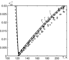
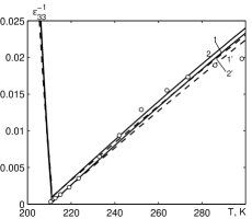
Figure 1: The temperature dependence of the inverse static dielectric permittivities of free $(\varepsilon^{\sigma}_{33})^{-1}$ and clamped $(\varepsilon^{\varepsilon}_{33})^{-1}$ K(H_1-xD${}_{x})_{2}$PO₄ crystals at $x=0.0$. Symbols are experimental data taken from $\circ$, $\bullet$ – [19], $\square$ – [20], $\lozenge$ – [21], $\triangleright$ – [22], $\triangleleft$ – [15], $\triangledown$ – [23], $\vartriangle$[24]. Solid lines: the present theory; dashed lines: the theoretical results of [11] for $(\varepsilon^{\sigma}_{33})^{-1}$ (1’) and $(\varepsilon^{\varepsilon}_{33})^{-1}$ (2’).

Figure 2: The same for $x=0.88$. Symbols are experimental data taken from $\circ$ – [25].

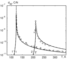
Figure 3: The temperature dependence of the piezoelectric coefficient $d_{36}$ of K(H_1-xD${}_{x})_{2}$PO₄ at $x=0.0$ – 1, 1’, $\square$ [19], $\triangledown$ [26], $\triangleright$, [27]; at $x=0.88$ – 2, 2’, $\circ$ [25]. Dashed lines: the theoretical results of [11].

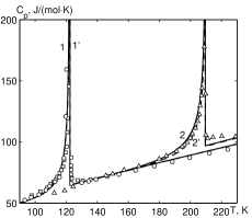
Figure 4: The temperature dependence of the molar specific heat of K(H_1-xD${}_{x})_{2}$PO₄ at $x=0.0$ – $\circ$ [17], $\square$ [18]; at $x=0.86$ – $\bigtriangleup$ [18]. Dashed lines: the theoretical results of [11].

However, the present model allows us to describe more consistently the smearing of the first order phase in high electric fields. In figs. 5, 6, and 7 we plotted the temperature variation of the polarization of K(H_1-xD${}_{x})_{2}$PO₄ in different fields.

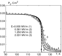
Figure 5: The temperature dependence of polarization of K(H_1-xD${}_{x})_{2}$PO₄ at $x=0$ and at different $E_{3}$(MV/m): 0.0 – 1, $\vartriangle$ [3]; 0.581 – 2, $\circ$[15]; 1.250 – 3, $\square$[15]; 2.031 – 4, $\lozenge$[15]. Symbols are experimental points; solid lines: the present theory; dashed lines: the theoretical results of [11].

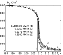
Figure 6: The temperature dependence of polarization of K(H_1-xD${}_{x})_{2}$PO₄ at $x=0.84$ and at different $E_{3}$(MV/m): 0.0 – 1; 0.625 – 2, $\circ$; 0.9375 – 3, $\square$; 1.25 – 4, $\lozenge$. Symbols are experimental points; lines: the present theory.

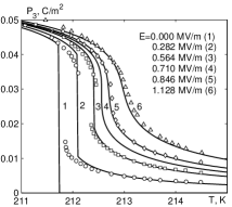
Figure 7: The temperature dependence of polarization of K(H_1-xD${}_{x})_{2}$PO₄ at $x=0.89$ and at different $E_{3}$ (MV/m): 0.0 – 1; 0.282 – 2, $\circ$; 0.564 – 3, $\square$; 0.71 – 4; 0.846 – 5, $\lozenge$; 1.128 – 6, $\vartriangle$. Symbols are experimental points taken from [16]; lines: the present theory.

The agreement with experiment is better at $x=0.84$ and 0.89 than at $x=0$. We believe this is due to proton tunnelling, essential in non-deuterated samples, which is not included in our model. The field $E_{3}$, which in these crystals is the field conjugate to the order parameter, induces non-zero polarization $P_{3}$ above the transition point. Polarization has a jump at $T_{c}$, indicating the first order phase transition. With increasing field, the polarization jump decreases, whereas the transition temperature $T_{c}$ increases almost linearly. The corresponding $\partial T_{c}/\partial E_{3}$ slopes are 0.192 and 0.115 K cm/kV for $x=0$ and $x=0.89$, respectively (c.f. 0.22 and 0.13 K cm/kV from our earlier calculations [8] and experimental $0.125$ K cm/kV of [29] for $x=0.89$). At some critical field $E^{*}$ the jump vanishes, and the transition smears out. The calculated coordinates of the critical point are $E^{*}=125$ V/cm, $T^{*}_{c}$=122.244 K for $x=0$ and $7.1$ kV/cm, 212.55 K for $x=0.89$, which agrees well with the experiment [28, 29]. It should be noted that in our previous calculations [11] it was impossible to obtain a correct description of the polarization behavior in the fields above the critical one, because of the necessity to use two different values of the effective dipole moment $\mu$ in calculations.

Smearing of the phase transition is observed also in the temperature dependences of the dielectric permittivity $\varepsilon_{33}$ (fig. 8), piezoelectric coefficient $d_{36}$ (fig. 9), and elastic constant $c_{66}^{E}$ (fig. 10).

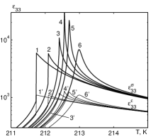
Figure 8: The temperature dependence of the inverse static dielectric permittivities of free $(\varepsilon^{\sigma}_{33})^{-1}$ (bold lines) and clamped $(\varepsilon^{\varepsilon}_{33})^{-1}$ (thin lines) K(H_1-xD${}_{x})_{2}$PO₄ crystals for $x=0.89$ at different electric fields $E_{3}$ (MV/m): 0.0 – 1, 1’; 0.282 – 2, 2’; 0.564 – 3, 3’; 0.71 – 4, 4’; 0.846 – 5, 5’; 1.128 – 6, 6’.

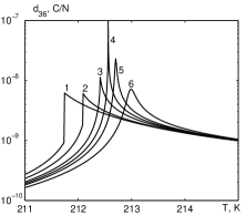
Figure 9: The temperature dependence of the piezoelectric coefficient $d_{36}$ of K(H_1-xD${}_{x})_{2}$PO₄ for $x=0.89$ at different electric fields $E_{3}$ (MV/m): 0.0 – 1, 1’; 0.282 – 2, 2’; 0.564 – 3, 3’; 0.71 – 4, 4’; 0.846 – 5, 5’; 1.128 – 6, 6’.

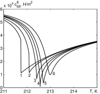
Figure 10: The temperature dependence of the elastic constant $c_{66}^{E}$ of K(H_1-xD${}_{x})_{2}$PO₄ for $x=0.89$ at different electric fields $E_{3}$ (MV/m): 0.0 – 1, 1’; 0.282 – 2, 2’; 0.564 – 3, 3’; 0.71 – 4, 4’; 0.846 – 5, 5’; 1.128 – 6, 6’.

The calculated changes of temperature $\Delta T$ of the KDP crystals with the adiabatically applied electric field is showin in figs. 12, 12, and 13.

Figure 11: The field dependences of the electrocaloric temperature change of K(H_1-xD${}_{x})_{2}$PO₄ for $x=0.0$ (solid lines) in the ferroelectric phase at $T-T_{c}^{0}=-2.04$ K – 1, $\square$ [3] and in the paraelectric phase at $T-T_{c}^{0}=3.28$ K – 2, $\circ$ [3]; for $x=0.89$ (dashed lines) $T-T_{c}^{0}=-2.04$ K – 1’ and $T-T_{c}^{0}$=3.28K – 2’.

Figure 12: The field dependence of the electrocaloric temperature change of K(H_1-xD${}_{x})_{2}$PO₄ at $T=T_{c}^{0}$ for $x=0.0$ (solid line, $\circ$ [5]) and $x=0.89$ (dashed line).

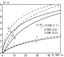
Figure 13: The field dependence of the electrocaloric temperature change of K(H_1-xD${}_{x})_{2}$PO₄ for $x=0.0$ (solid lines) and $x=0.89$ (dashed lines) at $T-T_{c}^{0}=-2.04$ K – 1, $1^{\prime}$; $T=T_{c}^{0}$ – 2, $2^{\prime}$; $T-T_{c}^{0}=3.2$ K – 3, $3^{\prime}$ for very high fields.

As one can see, at small fields (fig. 12) the calculated electrocaloric temperature change is a linear function of the field in the ferroelectric (curves 1, $1^{\prime}$) and a quadratic function in the paraelectric phase (curves 2, $2^{\prime}$). The experimental behavior in the ferroelectric phase is not linear at $E<3$ kV/cm because of the domains. The experimental data of [5] (fig. 12) were obtained at $T=121$ K, which was very close to the transition temperature of the sample used in the measurements. The domains, which polarization is oriented along the field, are heated, whereas the domains, polarized in the opposite direction are cooled. The disagreement between the theory and experiment for an undeuterated crystal in the ferroelectric phase can be also caused by tunneling, which is not taken into account in the present model. In very high fields (fig. 13) the calculated electrocaloric temperature change in the paraelectric phase are larger than in the ferroelectric phase. The obtained curves deviate from linear and quadratic behavior and reach saturation at $E\gg 50$ MV/m. To create fields that high in macroscopic single crystals is obviously practically impossible, because of the dielectric breakdown. However, experimental data for $\Delta T$ are not available even for moderate fields above 0.5 MV/m.

As one can see from the temperature dependence of $\Delta T$ (fig. 14), the calculated electrocaloric temperature change is the largest in the paraelectric phase close to $T_{c}$ and can exceed 6 K.

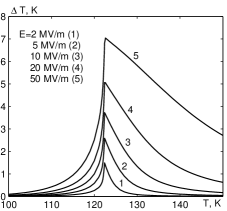
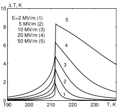
Figure 14: The temperature dependence of the electrocaloric temperature change of K(H_1-xD${}_{x})_{2}$PO₄ for $x=0.0$ (left) and $x=0.89$ (right) in different fields.

The electrocaloric effect in K(H_1-xD${}_{x})_{2}$PO₄ at $x=0.89$ is larger than at $x=0.0$, because with increasing deuteration the first order character of the phase transitions becomes more pronounced.

We can also find $\Delta T$ using Eq. (28), that is, as illustrated in fig. 15.

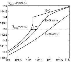
Figure 15: The temperature dependence of molar entropy of KDP at different fields.

The values of $\Delta T$ calculated using Eqs. (29) and (28) coincide.

4 Conclusions

Taking into account the dependence of the effective dipole moment on the order parameter allows us to correctly describe smearing of the ferroelectric phase transition in high electric field as well as the electrocaloric effect in KDP crystals. The theory predicts the values of the electrocaloric temperature change above 5 K in very high fields. This fact could make the KDP crystals a promising material for electrocaloric refridgerators. Additional experimental measurements of $\Delta T$ in fields above 0.5 MV/m are necessary.