A two-phase two-layer model for transdermal
drug delivery and percutaneous absorption

Abstract

One of the promising frontiers of bioengineering is the controlled release of a therapeutic drug from a vehicle across the skin (transdermal drug delivery). In order to study the complete process, a two-phase mathematical model describing the dynamics of a substance between two coupled media of different properties and dimensions is presented. A system of partial differential equations describes the diffusion and the binding/unbinding processes in both layers. Additional flux continuity at the interface and clearance conditions into systemic circulation are imposed. An eigenvalue problem with discontinuous coefficients is solved and an analytical solution is given in the form of an infinite series expansion. The model points out the role of the diffusion and reaction parameters, which control the complex transfer mechanism and the drug kinetics across the two layers. Drug masses are given and their dependence on the physical parameters is discussed.

Keywords: Diffusion-reaction equation, transdermal drug delivery, percutaneous absorption, binding – unbinding, local mass non-equilibrium.

1 Introduction

Transdermal drug delivery (TDD for short) is an approach used to deliver drugs through the skin for therapeutic purposes as an alternative to oral, intravascular, subcutaneous and transmucosal routes. Various TDD technologies are possible including the use of suitable drug formulations, carriers such as nanoparticles and penetration enhancers to facilitate drug delivery and transcutaneous absorption. TDD offers several advantages compared to other traditional delivery methods: controlled release rate, noninvasive administration, less frequent dosing, and simple application without professional medical aids, improving patient compliance. For these reasons it represents a valuable and attractive alternative to oral administration [1].

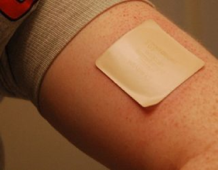
Figure 1: The transdermal patch, a typical vehicle in transdermal drug delivery.

Drugs can be delivered across the skin to have an effect on the tissues adjacent to the site of application (topical delivery) or to be effective after distribution through the circulatory system (systemic delivery). While there are many advantages to TDD, the skin’s barrier properties provide a significant challenge. To this aim, it is important to understand the mechanism of drug permeation from the delivery device (or vehicle, typically a transdermal patch or medicated plaster, fig. 1) across the skin [2]. In TDD, the drug should be absorbed to an adequate extent and rate in order to achieve and maintain uniform, systemic, effective levels throughout the duration of use. TDD must be carefully tailored to achieve the optimal therapeutic effect and to deliver the correct dose in the required time [3]. The pharmacological effects of the drug, tissue accumulation, duration and distribution could potentially have an effect on its efficacy and a delicate balance between an adequate amount of drug delivered over an extended period of time and the minimal local toxicity should be found [4]. Most drugs do not penetrate skin at rates sufficient for therapeutic efficacy and this restrictive nature limits the use of the transdermal route to molecules of low molecular weight and with moderate lipophilicity. In general, the first skin layer, the stratum corneum, presents most of the resistance to diffusive transport into skin. Thus, once the drug molecules cross it, transfer into deeper dermal layers and systemic uptake occurs in a relatively short time. In order to speed up transdermal permeation of drugs in the stratum corneum, new delivery techniques are currently under investigation, for example the use of chemical enhancers or microneedles and techniques such as ultrasound, electroporation and iontophoresis [3, 5].

Mathematical modelling for TDD constitutes a powerful predictive tool for the fundamental understanding of biotransport processes, and for screening processes and stability assessment of new formulations. In the absence of experiments, a number of mathematical models and numerical simulations have been carried out regarding TDD, its efficacy and the optimal design of devices [6, 7, 8, 9]. Recent extensive reviews deal with various aspects of transdermal delivery at different scales [2, 10, 11, 12]. In general, drug absorption into the skin occurs by passive diffusion and most of the proposed models consider this effect only. On the other hand, there is a limited effort to explain the drug delivery mechanism from the vehicle platform. This is a very important issue indeed, since the polymer matrix acts as a drug reservoir, and an optimal design of its microstructural characteristics would improve the release performances [13]. For example, in the vehicle, the dissolution of the drug from encapsulated to free phase occurs at a given reaction rate. Another relevant feature in TDD is the similar binding/unbinding process through the receptor sites in the skin. These drug association-dissociaton aspects are often neglected or underestimated by most authors who consider purely diffusive systems in the skin or in the vehicle [20, 21]. One exception is the work of Anissimov et al.[2, 4], where a linear reversible binding is considered, but the vehicle is taken into account only through a boundary condition of the first kind. However, it is worth emphasizing that the drug elution depends on the properties of the “vehicle-skin” system, taken as a whole, and modelled as a coupled two-layered system.

The method used in the present study follows the mathematical approach developed in a series of previously published papers which successfully describe drug dynamics form an eluting stent embedded in an arterial wall [14–17]. In these papers, we proposed a number of models of increasing complexity to explain the diffusion-advection-reaction release mechanism of a drug from the stent coating to the wall, constituted of a number of contiguous homogeneous media of different properties and extents. Separation of variables leads to an eigenvalue problem with discontinuous coefficients and an exact solution is given in terms of infinite series expansion and is based on a two- or multi-layer diffusion model. In the wake of these papers, a two-layer two-phase coupled model for TDD has been recently presented and a semi-analytical solution has been proposed for drug concentration and mass in the vehicle and the skin at various times, for special values of the parameters [18].

In the present paper we extend the above study and remove some of the simplifying assumptions, obtaining a solution in a more general form. Together with diffusive effects, the drug dissolution process in the polymer constituting the vehicle platform and the reversible drug binding process in the skin are also addressed. A solution of the Fick-type reaction-diffusion equations (reduced problem) serves as the building block to construct a space-time dependent solution for the general equations (full problem). A major issue in modelling TDD is the assessment of the key parameters defining skin permeability, diffusion coefficients, drug dissociation and association rates. Lacking experimental data and reliable estimates of the model parameters, we carry out a systematic sensitivity analysis over a feasible range of parameter values. The results of the simulations provide valuable insights into local TDD and can be used to assess experimental procedures to evaluate drug efficacy, for an optimal control strategy in the design of technologically advanced transdermal patches.

2 Formulation of the problem

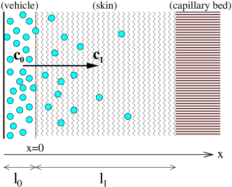
Figure 2: Cross-section of the vehicle and the skin layers, geometrical configuration and reference system in TDD. Due to an initial difference of free drug concentrations $c_{0}$ and $c_{1}$, a mass flux is established at the interface and drug diffuses through the skin. At a distance $x=l_{1}$ the skin-receptor (capillary bed) is present where all drug is assumed to be absorbed. Figure not to scale.

To model TDD, let us consider a two-layered system composed of: (i) the vehicle (the transdermal patch or the film of an ointment), and (ii) the skin (the stratum corneum followed by the skin-receptor cells and the capillary bed) (fig. 2). The drug is stored in the vehicle, a reservoir consisting of a polymeric matrix. This is enclosed on one side with an impermeable backing and having on the other side an adhesive in contact with the skin. A rate-controlling membrane protecting the polymer matrix may exist. In this configuration, the first layer is shaped as a planar slab that is in direct contact with the skin, the second layer. As most of the mass dynamics occurs along the direction normal to the skin surface, we restrict our study to a simplified one-dimensional model. In particular, we consider as $x$-axis the normal to the skin surface and oriented with the positive direction outwards the skin. Without loss of generality, let $x_{0}=0$ be the vehicle-skin interface and $l_{0}$ and $l_{1}$ the thicknesses of the vehicle and skin layers respectively (fig. 2). The vehicle and the skin are both treated from a macroscopic perspective so that they are represented as two homogeneous media.

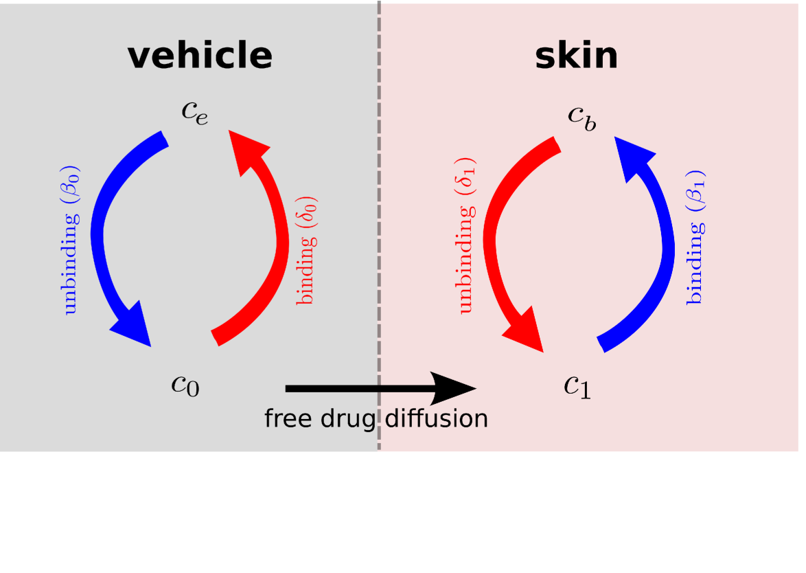
Figure 3: A diagram sketching the cascade mechanism of drug delivery and percutaneous absorption in the vehicle-skin coupled system. A unbinding (resp. binding) reaction occurs in the vehicle (resp. in the skin) (blue arrows). In both layers, reverse reactions (red arrows) are present in a dynamic equilibrium. Drug diffusion occurs only in the free phases $c_{0}$ and $c_{1}$.

Initially, the drug is encapsulated at maximum concentration within the vehicle in a bound phase (e.g. nanoparticles or crystalline form) ($c_{e}$): in a such state, it is unable to be delivered to the tissue. Then, a fraction of this drug ($\beta_{0}c_{e}$) is transferred, through an unbinding process, to an unbound – free, biologically available – phase ($c_{0}$), and conversely, a part of the free drug ($\delta_{0}c_{0}$) is transferred by a binding process to the bound state, in a dynamic equilibrium (fig. 3). Also, at the same time, another fraction of free drug ($c_{1}$) begins to diffuse into the adjacent skin (delivery). Similarly, in the skin – the release medium – a part of the unbound drug ($\beta_{1}c_{1}$) is metabolized by the cell receptors and transformed in a bound state ($c_{b}$) (absorption), and with the reverse unbinding process ($\delta_{1}c_{b}$) again in a unbound phase. Thus, the drug delivery-absorption process starts from the vehicle and ends to the skin receptors, with bidirectional phase changes in a cascade sequence, as schematically represented in fig. 3. Local mass non-equilibrium processes, such as bidirectional drug binding/unbinding phenomena, play a key role in TDD, with characteristic times faster than those of diffusion. In other cases of drug delivery, such as in eluting stents, a second-order saturable reversible binding model has been proposed [19]: this comprehensive model includes a number of drug dependent parameters which are difficult to measure experimentally and, nevertheless, does not necessarily apply to TDD. Here, a linear relationship is commonly used, as the density of binding sites far exceeds the local free drug concentration [2, 4]. In the first layer the process is described by the following equations:

$${\partial c_{e}\over\partial t}=-\beta_{0}c_{e}+\delta_{0}c_{0} \mbox{in}\,(-l_{0},0)\,\,$$ (2.1)

$${\partial c_{0}\over\partial t}=D_{0}{\partial^{2}c_{0}\over\partial x^{2}}+\beta_{0}c_{e}-\delta_{0}c_{0} \mbox{in}\,(-l_{0},0)\,\,$$ (2.2)

where $D_{0}$ ($cm^{2}/s$) is the effective diffusion coefficient of the unbound solute, $\beta_{0}\geq 0$ and $\delta_{0}\geq 0$ ($s^{-1}$) are the unbinding and binding rate constants in the vehicle, respectively. In detail, the rate of release of encapsulated drug into its free state is implied by the dissociation rate constant $\beta_{0}$, while $\delta_{0}$ provides a representation of the rate at which the free solute re-associates in the bound state.

Similarly, in the second layer, the drug dynamics is governed by similar reaction-diffusion equations:

$${\partial c_{1}\over\partial t}=D_{1}{\partial^{2}c_{1}\over\partial x^{2}}-\beta_{1}c_{1}+\delta_{1}c_{b} \,\,(0,l_{1})$$ in (2.3)

$${\partial c_{b}\over\partial t}=\beta_{1}c_{1}-\delta_{1}c_{b} \,\,(0,l_{1})$$ in (2.4)

where $D_{1}$ is the effective diffusivity of unbound drug, $\beta_{1}\geq 0$ and $\delta_{1}\geq 0$ are the binding and unbinding rate constants in the skin, respectively, defined similarly as above for the vehicle. They can be evaluated experimentally as described in [4, 9], sometimes through the equilibrium dissociation constant $K=\displaystyle{\delta_{1}\over\beta_{1}}$. The magnitudes of $\delta_{1}$ and $\beta_{1}$ are inversely proportional to the typical times associated with the binding-unbinding processes. However, these reaction times are not negligible compared with the diffusive characteristic times (slow binding) [11].

To close the previous bi-layered mass transfer system of eqns. (2.1)–(2.4), a flux continuity condition has to be assigned at the vehicle-skin interface:

$$-D_{0}{\partial c_{0}\over\partial x}=-D_{1}{\partial c_{1}\over\partial x}\qquad\mbox{at}\,\,x=0$$ (2.5)

As far as the concentration continuity is concerned, this is not guaranteed because of a different drug partitioning between vehicle and skin. This is taken into account through an appropriate mass transfer coefficient $P_{r}$ [9, 11]. Additionally, a semi-permeable rate-controlling membrane or an adhesive film or a non-perfect vehicle-skin contact, having $1/P_{m}$ as mass resistance, might be present at the interface. Thus, a jump concentration may occur:

$$-D_{1}{\partial c_{1}\over\partial x}=P(c_{0}-c_{1})\qquad\mbox{at}\,\,x=0$$ (2.6)

with $P(cm/s)$ the overall mass transfer coefficient :

$${1\over P}={1\over P_{r}}+{1\over P_{m}}$$

Estimation of the partition coefficient or of its derived quantity $P_{r}$ is a very difficult task. The recent review of Mitragotri et al. [2] provides an excellent overview of the current methods used for its representation. The usually met condition $c_{0}\propto c_{1}$ does not apply, in our opinion, to time dependent cases.

No mass flux passes between the vehicle and the external surrounding due to the impermeable backing and we impose a no-flux condition :

$$D_{0}{\partial c_{0}\over\partial x}=0\qquad\qquad\mbox{at $x=-l_{0}$}$$ (2.7)

Finally, a boundary condition has to be imposed at the skin-receptor (capillary) boundary. At this point the elimination of drug by capillary system follows first-order kinetics:

$$K_{cl}c_{1}+D_{1}{\partial c_{1}\over\partial x}=0\qquad\qquad\qquad\mbox{at }x=l_{1}$$ (2.8)

where $K_{cl}$ is the skin-capillary clearance per unit area ($cm/s$). The initial conditions are:

$$c_{e}(x,0)=C_{e}\qquad\qquad c_{0}(x,0)=0\qquad\qquad c_{1}(x,0)=0\qquad\qquad c_{b}(x,0)=0$$ (2.9)

2.1 Dimensionless equations

All the variables and the parameters are now normalized to get easily computable dimensionless quantities as follows:

$$\bar{x}={x\over l_{1}}\qquad\qquad\bar{t}={D_{1}\over(l_{1})^{2}}t\qquad\qquad\phi={Pl_{1}\over D_{1}}$$

$$\bar{l}_{0}={l_{0}\over l_{1}}\qquad\qquad\gamma={D_{0}\over D_{1}}\qquad\qquad\bar{c}_{i}={c_{i}\over C_{e}}$$

$$K={K_{cl}l_{1}\over D_{1}}\qquad\qquad\bar{\beta}_{i}={\beta_{i}(l_{1})^{2}\over D_{1}}\qquad\qquad\bar{\delta}_{i}={\delta_{i}(l_{1})^{2}\over D_{1}}\qquad i=0,1$$

By omitting the bar for simplicity, the mass transfer problem (2.1)–(2.4) can be now written in dimensionless form as:

$${\partial c_{e}\over\partial t}=-\beta_{0}c_{e}+\delta_{0}c_{0} \mbox{in}\,(-l_{0},0)\,\,$$ (2.10)

$${\partial c_{0}\over\partial t}=\gamma{\partial^{2}c_{0}\over\partial x^{2}}+\beta_{0}c_{e}-\delta_{0}c_{0} \mbox{in}\,(-l_{0},0)\,\,$$ (2.11)

$${\partial c_{1}\over\partial t}={\partial^{2}c_{1}\over\partial x^{2}}-\beta_{1}c_{1}+\delta_{1}c_{b} \mbox{in}\,\,(0,1)$$ (2.12)

$${\partial c_{b}\over\partial t}=\beta_{1}c_{1}-\delta_{1}c_{b} \mbox{in}\,\,(0,1)$$ (2.13)

and the interface and boundary conditions (2.5)–(2.8) read:

$${\partial c_{0}\over\partial x}=0 \,\,x=-l_{0}$$ at

$$\gamma{\partial c_{0}\over\partial x}={\partial c_{1}\over\partial x}\qquad\qquad-{\partial c_{1}\over\partial x}=\phi(c_{0}-c_{1}) \>\>x=0$$ at

$$Kc_{1}+{\partial c_{1}\over\partial x}=0 \,\,x=1$$ at (2.14)

supplemented with the initial condition:

$$c_{e}(x,0)=1\qquad\qquad c_{0}(x,0)=0\qquad\qquad c_{1}(x,0)=0\qquad\qquad c_{b}(x,0)=0$$ (2.15)

3 Solving a reduced problem

To solve the above problem, let us consider, preliminarily, the associated system of P.D.E.’s obtained from (2.11)–(2.12) by setting $c_{e}=c_{b}=0$:

$${\partial\tilde{c}_{0}\over\partial t}=\gamma{\partial^{2}\tilde{c}_{0}\over\partial x^{2}}-\delta_{0}\tilde{c}_{0}\qquad\qquad-l_{0}<x<0$$

$${\partial\tilde{c}_{1}\over\partial t}={\partial^{2}\tilde{c}_{1}\over\partial x^{2}}-\beta_{1}\tilde{c}_{1}\qquad\qquad 0<x<1$$ (3.1)

with the same boundary conditions (2.14) and homogeneous initial conditions. We look for a non trivial solution by separation of variables:

$$\tilde{c}_{0}(x,t)=X_{0}(x)G_{0}(t)\qquad\qquad\tilde{c}_{1}(x,t)=X_{1}(x)G_{1}(t)$$ (3.2)

After substitution, eqns.(3.1) become:

$$\left({dG_{0}\over dt}+\delta_{0}G_{0}\right)X_{0}=\gamma X_{0}^{\prime\prime}G_{0}\qquad-l_{0}<x<0$$

$$\left({dG_{1}\over dt}+\beta_{1}G_{1}\right)X_{1}=X_{1}^{\prime\prime}G_{1}\qquad 0<x<1$$ (3.3)

From the previous, $X_{0}$ and $X_{1}$ must satisfy the spatial eigenvalue problem:

$$X_{0}^{\prime\prime}=-\lambda_{0}^{2}X_{0}\qquad-l_{0}<x<0$$

$$X_{1}^{\prime\prime}=-\lambda_{1}^{2}X_{1}\qquad 0<x<1$$ (3.4)

with:

$$X_{0}^{\prime}=0 \,\,x=-l_{0}$$ at

$$\gamma{X_{0}^{\prime}}={X_{1}^{\prime}}\qquad\qquad-{X_{1}^{\prime}}=\phi(X_{0}-X_{1}) \>\>x=0$$ at

$$KX_{1}+{X^{\prime}_{1}}=0 \,\,x=1$$ at (3.5)

The eigenfunctions of the problem (3.4) are searched as:

$$X_{0}(x)=a_{0}\cos(\lambda_{0}x)+b_{0}\sin(\lambda_{0}x)\qquad\qquad X_{1}(x)=a_{1}\cos(\lambda_{1}x)+b_{1}\sin(\lambda_{1}x)$$ (3.6)

By enforcing the conditions (3.5), we get the following linear system of equations:

$$\left\{\begin{array}[]{l}a_{0}\sin(\lambda_{0}l_{0})+b_{0}\cos(\lambda_{0}l_{0})=0\\[14.22636pt] \gamma\lambda_{0}b_{0}=\lambda_{1}b_{1}\\[14.22636pt] \phi(a_{0}-a_{1})+\lambda_{1}b_{1}=0\\[14.22636pt] \left[K\cos(\lambda_{1})-\lambda_{1}\sin(\lambda_{1})\right]a_{1}+\left[K\sin(\lambda_{1})+\lambda_{1}\cos(\lambda_{1})\right]b_{1}=0\end{array}\right.$$

A non trivial solution ($a_{0},b_{0},a_{1},b_{1}$) with:

$$a_{0}=a_{1}-{\lambda_{1}\over\phi}b_{1}=-b_{0}\cot(\lambda_{0}l_{0})$$

$$b_{0}={\lambda_{1}\over\gamma\lambda_{0}}\>b_{1}$$

$$a_{1}={K\tan\lambda_{1}+\lambda_{1}\over\lambda_{1}\tan\lambda_{1}-K}b_{1}$$ (3.7)

and $b_{1}$ arbitrary, exists only if the determinant of the coefficient matrix is zero, i.e.:

$$\lambda_{1}\left(\lambda_{1}\tan(\lambda_{1})-K\right)\left[\gamma\lambda_{0}\tan(\lambda_{0}l_{0})-\phi\right]-\gamma\phi\lambda_{0}\tan(\lambda_{0}l_{0})\left(K\tan(\lambda_{1})+\lambda_{1}\right)=0$$ (3.8)

In general, the transcendental eqn (3.8) admits infinite eigenvalues. On the other hand, from (3.3), we have:

$${dG_{0}\over dt}+(\delta_{0}+\gamma\lambda_{0}^{2})G_{0}=0$$

$${dG_{1}\over dt}+(\beta_{1}+\lambda_{1}^{2})G_{1}=0$$ (3.9)

In order to satisfy the matching conditions at the interface $x=0$ for all $t>0$, from (3.9) it follows:

$$G(t)\equiv G_{0}(t)=G_{1}(t)=\exp(-\omega t)$$

with

$$\omega\equiv\delta_{0}+\gamma\lambda_{0}^{2}=\beta_{1}+\lambda_{1}^{2}$$ (3.10)

From the latter, it follows:

$$\lambda_{0}=\sqrt{\lambda_{1}^{2}+\beta_{1}-\delta_{0}\over\gamma}$$ (3.11)

and replacing in (3.8) we get a set of eigenvalues ($\lambda_{0}^{k},\lambda_{1}^{k}$) and of eigenvectors ($X_{0}^{k},X_{1}^{k}$) as in eqn. (3.6). Note that, although from eqn. (3.11) some eigenvalues can be imaginary, this circumstance is excluded with the numerical values used (see sect. 5). We can easily prove that ($X_{0}^{k},X_{1}^{k}$) form a orthogonal system, that is:

$$\int\limits^{0}_{-l_{0}}X_{0}^{k}X_{0}^{q}dx+\int\limits^{1}_{0}X_{1}^{k}X_{1}^{q}dx=\left\{\begin{array}[]{lll}0&\mbox{for}&k\neq q\\[7.11317pt] N_{k}&\mbox{for}&k=q\end{array}\right.$$ (3.12)

where

$$N_{k} = {1\over 2}\left[\left((a_{0}^{k})^{2}+(b_{0}^{k})^{2}\right)l_{0}-{a_{0}^{k}b_{0}^{k}\over\lambda_{0}^{k}}+(a_{1}^{k})^{2}+1+{a_{1}^{k}\over\lambda_{1}^{k}}\right]$$ (3.13)

Finally the concentrations are expressed by summing up all the contributions:

$$\tilde{c}_{0}(x,t)=\sum\limits_{k=1}^{\infty}X_{0}^{k}(x)G^{k}(t)\qquad\qquad\tilde{c}_{1}(x,t)=\sum\limits_{k=1}^{\infty}X_{1}^{k}(x)G^{k}(t)$$ (3.14)

4 Solution of the full problem

Consider first that, by making explicit $c_{e}$ from eqn. (2.10), $c_{b}$ from eqn. (2.13), and from initial conditions (2.15), we have

$$c_{e}(x,t)=\exp(-\beta_{0}t)+\delta_{0}\int\limits^{t}_{0}c_{0}(x,\tau)\exp[\beta_{0}(\tau-t)]d\tau$$ (4.1)

$$c_{b}(x,t)=\beta_{1}\int\limits^{t}_{0}c_{1}(x,\tau)\exp[\delta_{1}(\tau-t)]d\tau$$ (4.2)

The eqns. (4.1)–(4.2) mean that $c_{e}$ (resp. $c_{b}$) are computed in terms of $c_{0}$ (resp. $c_{1}$) and the latter are expressed in the space spanned by $X_{0}^{k}$ (resp. $X_{1}^{k}$) (see eqn. (3.6)), with the set of eigenvalues and eqn. (3.10) unchanged, similarly to eqn. (3.14), as:

$$c_{0}(x,t)=\sum\limits_{k=1}^{\infty}X_{0}^{k}(x)U^{k}(t)\qquad\qquad c_{1}(x,t)=\sum\limits_{k=1}^{\infty}X_{1}^{k}(x)U^{k}(t)$$ (4.3)

where the time functions $U^{k}(t)$ have to be computed for the complete system (2.10)–(2.13). Replacing (4.3), eqns. (4.1)-(4.2) are written as:

$$c_{e}(x,t)=\exp(-\beta_{0}t)+\delta_{0}\sum\limits_{k=1}^{\infty}X_{0}^{k}(x)H_{0}^{k}(t)\qquad\qquad c_{b}(x,t)=\beta_{1}\sum\limits_{k=1}^{\infty}X_{1}^{k}(x)H_{1}^{k}(t)$$ (4.4)

with

$$H_{0}^{k}(t)=\int\limits_{0}^{t}U^{k}(\tau)\exp[\beta_{0}(\tau-t)]d\tau\qquad\qquad H_{1}^{k}(t)=\int\limits_{0}^{t}U^{k}(\tau)\exp[\delta_{1}(\tau-t)]d\tau$$ (4.5)

By inserting (4.3)–(4.4) into eqn. (2.11), multiplying by $X_{0}^{p}$, we get:

$$\sum\limits_{k=1}^{\infty}X_{0}^{k}X_{0}^{p}{dU^{k}\over dt}=-\gamma\sum\limits_{k=1}^{\infty}X_{0}^{k}X_{0}^{p}(\lambda_{0}^{k})^{2}U^{k}-\delta_{0}\sum\limits_{k=1}^{\infty}X_{0}^{k}X_{0}^{p}U^{k}$$

$$+\beta_{0}\exp(-\beta_{0}t)X_{0}^{p}+\beta_{0}\delta_{0}\sum\limits_{k=1}^{\infty}X_{0}^{k}X_{0}^{p}H_{0}^{k}$$ (4.6)

Similarly, multiplying eqn. (2.12) by $X_{1}^{p}$, we have:

$$\sum\limits_{k=1}^{\infty}X_{1}^{k}X_{1}^{p}{dU^{k}\over dt}=-\sum\limits_{k=1}^{\infty}X_{1}^{k}X_{1}^{p}(\lambda_{1}^{k})^{2}U^{k}-\beta_{1}\sum\limits_{k=1}^{\infty}X_{1}^{k}X_{1}^{p}U^{k}+\beta_{1}\delta_{1}\sum\limits_{k=1}^{\infty}X_{1}^{k}X_{1}^{p}H_{1}^{k}$$ (4.7)

Integrating the previous eqns over the corresponding layers and summing up, we get:

$$\sum\limits_{k=1}^{\infty}{dU^{k}\over dt}\left(\int\limits_{-l_{0}}^{0}X_{0}^{k}X_{0}^{p}dx+\int\limits_{0}^{1}X_{1}^{k}X_{1}^{p}dx\right)=-\sum\limits_{k=1}^{\infty}U^{k}\left(\gamma(\lambda_{0}^{k})^{2}\int\limits_{-l_{0}}^{0}X_{0}^{k}X_{0}^{p}dx+(\lambda_{1}^{k})^{2}\int\limits_{0}^{1}X_{1}^{k}X_{1}^{p}dx\right)$$

$$-\delta_{0}\sum\limits_{k=1}^{\infty}U^{k}\int\limits_{-l_{0}}^{0}X_{0}^{k}X_{0}^{p}dx-\beta_{1}\sum\limits_{k=1}^{\infty}U^{k}\int\limits_{0}^{1}X_{1}^{k}X_{1}^{p}dx$$

$$+\beta_{0}\exp(-\beta_{0}t)\int\limits_{-l_{0}}^{0}X_{0}^{p}dx+\beta_{0}\delta_{0}\sum\limits_{k=1}^{\infty}H_{0}^{k}\int\limits_{-l_{0}}^{0}X_{0}^{k}X_{0}^{p}dx+\beta_{1}\delta_{1}\sum\limits_{k=1}^{\infty}H_{1}^{k}\int\limits_{0}^{1}X_{1}^{k}X_{1}^{p}dx$$ (4.8)

We now pose:

$$\theta^{p}_{0}=\int\limits_{-l_{0}}^{0}X_{0}^{p}(x)dx=-{b_{0}^{p}\over\lambda_{0}^{p}}$$ (4.9)

$$\alpha_{0}^{kp}=\int\limits_{-l_{0}}^{0}X_{0}^{p}(x)X_{0}^{k}(x)dx\qquad\qquad\alpha_{1}^{kp}=\int\limits_{0}^{1}X_{1}^{p}(x)X_{1}^{k}(x)dx$$ (4.10)

Note that the space integrated constants $\theta^{p}_{0}$ and $\alpha_{0}^{kp}$ are the same as those computed in Ref. [17], and, from the orthogonality condition (3.12), they satisfy:

$$\alpha_{0}^{kp}+\alpha_{1}^{kp}=\left\{\begin{array}[]{lll}0&\mbox{for}&k\neq p\\[7.11317pt] N_{k}&\mbox{for}&k=p\end{array}\right.$$ (4.11)

By means of eqn. (3.10), the manipulation of eqn. (4.8) yields:

$$\begin{array}[]{l}\displaystyle{dU^{p}\over dt}+\omega^{p}U^{p}=\frac{1}{N_{p}}\left(\beta_{0}\exp(-\beta_{0}t)\theta^{p}_{0}+\beta_{0}\delta_{0}\sum\limits_{k=1}^{\infty}H_{0}^{k}\alpha_{0}^{kp}+\beta_{1}\delta_{1}\sum\limits_{k=1}^{\infty}H_{1}^{k}\alpha_{1}^{kp}\right)\end{array}$$ (4.12)

From eqn (4.5), $H_{0}^{p}(t)$ and $H_{1}^{p}(t)$ can be computed via the Leibnitz rule as:

$$\begin{array}[]{l}\displaystyle{dH_{0}^{p}\over dt}+\beta_{0}H_{0}^{p}=U^{p}\\[14.22636pt] \displaystyle{dH_{1}^{p}\over dt}+\delta_{1}H_{1}^{p}=U^{p}\end{array}$$ (4.13)

The system of the three ODE’s (4.12)–(4.13), with homogeneous initial conditions:

$$U^{p}(0)=H_{0}^{p}(0)=H_{1}^{p}(0)=0$$ (4.14)

is solved numerically with an explicit Runge-Kutta type solver with an adaptive time step. The obtained functions $U^{p}$, $H_{0}^{p}$ and $H_{1}^{p}$ allow the computation of all concentrations in eqns. (4.3)–(4.4).

From the analytical form of the solution given by eqns. (4.4) the drug masses are easily computed as integrals of the concentrations over the correspondent layer:

$$M_{j}(t)=\int\limits c_{j}(x,t)dx\qquad\qquad j=e,0,1,b$$ (4.15)

Furthermore, the fraction of drug mass retained in each layer and phase is computed as:

$$\mu_{j}(t)={M_{j}(t)\over M_{e}(0)}\qquad\qquad j=e,0,1,b$$ (4.16)

These are useful indicators of the drug released, diffused and absorbed during time.

5 Numerical simulations and results

A common difficulty in simulating physiological processes is the identification of reliable estimates of the model parameters. Experiments of TDD are impossible or prohibitively expensive in vivo and the only available source are lacking and incomplete data from literature. The physical problem depends on a large number of parameters, each of them may vary in a finite range, with a variety of combinations and limiting cases. The model constants cannot be chosen independently from each other and there is a compatibility condition among them. In this paper, for simplicity, the following physical parameters are kept fixed for simulations in TDD [4, 11, 20, 21]:

$$D_{0}=5\cdot 10^{-7}cm^{2}/s\qquad D_{1}=7\cdot 10^{-8}cm^{2}/s\qquad P=10^{-6}cm/s\qquad K_{cl}=3\cdot 10^{-3}cm/s$$ (5.1)

and the binding/unbinding parameters are varied to study the effect and to quantify the sensitivity of the delivery system, with the condition that the characteristic reaction times are smaller than the diffusion times, i.e.: $\beta_{0}>\displaystyle{D_{0}\over l_{0}^{2}}$ and $\beta_{1}>\displaystyle{D_{1}\over l_{1}^{2}}$.

The thickness of the vehicle is set as $l_{0}=40\mu m$, whereas the limit of the skin layer ($l_{1}$) is estimated by the following considerations. Strictly speaking, in a diffusion-reaction problem the concentration vanishes asymptotically at infinite distance. However, for computational purposes, the concentration is damped out (within a given tolerance) over a finite distance at a given time. Such a length (named penetration distance, see [16]) critically depends on the diffusive properties of the two-layered medium and, in particular, is related to the ratio $\displaystyle{D_{0}\over D_{1}}$. In our case, $l_{1}$ falls beyond the stratum corneum thickness, say $l_{1}=0.1cm$.

All the series appearing in the solution (4.4) and following, have been truncated at a number of 40 terms.

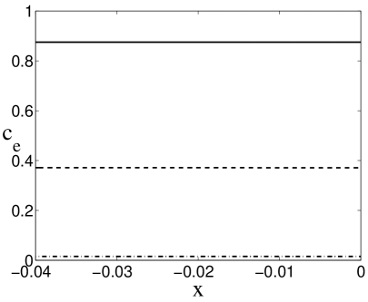
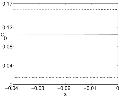
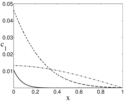
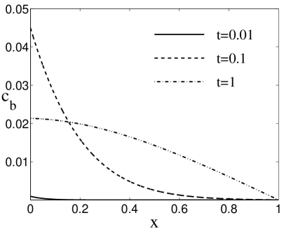
Figure 4: Concentration profiles in the vehicle ($c_{e}$ and $c_{0}$ above) and in the skin ($c_{1}$ and $c_{b}$ below) for the following dimensional binding/unbinding parameters ($s^{-1}$): $\beta_{0}=10^{-4},\beta_{1}=1.5\cdot 10^{-4},\delta_{0}=10^{-4},\delta_{1}=10^{-4}$, at three times (note the different scale of concentrations between the two layers).

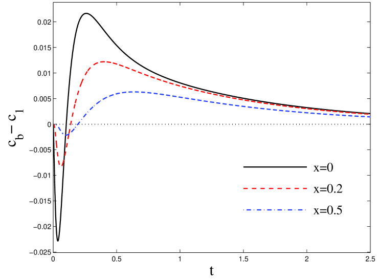
Figure 5: Difference between bound and free concentrations $c_{e}-c_{0}$ (top) and $c_{b}-c_{1}$ (bottom) as a function of time for the same binding-unbinding parameters of fig. 4. In the vehicle a fast decaying phase transfer is evidenced. Due to its thin size, this phase transition $c_{e}\rightarrow c_{0}$ occurs at the same manner at any location, whereas in the skin it is shown the larger amount of drug phase change at locations near the interface $x=0$.

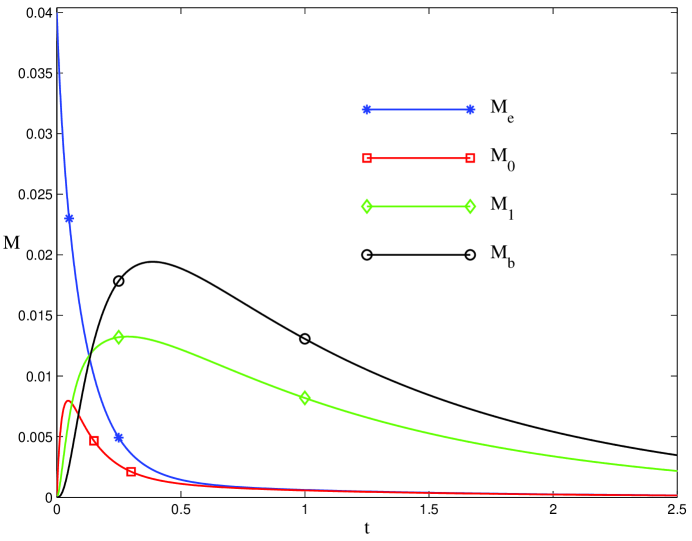
Figure 6: Time histories of the drug mass in the vehicle ($M_{e}$ and $M_{0}$) and in the skin ($M_{1}$ and $M_{b}$) for the same binding-unbinding parameters of fig. 4. Only $M_{e}$ exhibits an exponential decay, whereas $M_{0},M_{1}$ and $M_{b}$ increase at initial times, reach a peak $M^{*}$ at time $t^{*}$, and then damp to zero at a given rate.

The concentration profiles are almost flat in the vehicle, because of its small size, are discontinuous at the interface, and have a space decreasing behavior at any time in the skin layer, damping out within the penetration distance at all times (fig. 4). In the skin, a fast phase exchange of drug occurs at early times, more evident in regions close to the interface $x=0$, and continues at later times (fig. 5). The mass $M_{e}$ is decreasing in the vehicle, and $M_{0}$ (resp. $M_{1},M_{b}$), is first increasing up to some upper bound $M_{0}^{*}$ (resp. $M_{1}^{*},M_{b}^{*}$) (at a time $t_{0}^{*}$ (resp. $t_{1}^{*},t_{b}^{*}$), with $t_{0}^{*}<t_{1}^{*}<t_{b}^{*}$) and then decaying asymptotically with time (fig. 6).

The effect of binding/unbinding is studied by varying systematically the values of the on-off reaction rates $\beta_{0},\beta_{1},\delta_{0},\delta_{1}$ over an extended range (this is made feasible by setting the other parameters as in eqn. (5.1)). One parameter is changed at a time, letting the others fixed. The occurrence and the magnitude of the drug peak as well as the time scale of the absorption process result to be very sensitive to the mutual size of reaction parameters, combined with those of diffusive coefficients. In tables 1-4 these values are reported for a number of cases.

Effect of $\beta_{0}$ and $\delta_{0}$ (tables 1 and 2).
Small values of $\beta_{0}$ make the dissolution process slower. In the limit $\beta_{0}\rightarrow 0$ all drug tends to remain in the phase $c_{e}$ and it is hardly released and absorbed. For $\beta_{0}$ large, the phenomenon is characterized by marked peaks at early instants. On the other hand, for a fixed $\beta_{0}$, the TDD can be greatly influenced by the possible drug re-association. For a large $\delta_{0}$ the release is slowed down and the drug levels appear to be more uniform, with lower peak values.

Effect of $\beta_{1}$ and $\delta_{1}$ (tables 3 and 4).
In the second layer, the variation of $\beta_{1}$ and $\delta_{1}$ influences only the mass $M_{1}$ and especially $M_{b}$, letting the dynamics of $c_{e}$ and $c_{0}$ unchanged. A small $\beta_{1}$ is responsible for a raise of $M_{1}$, leaving $M_{b}$ small. For a $\beta_{1}$ sufficiently large (in our simulations $\approx 2\cdot 10^{-4}s^{-1}$) bound drug tends to accumulate at a much greater rate than it can be transferred from the contiguous layer and the process cannot be sustained by this value. For small values of $\delta_{1}$ the replenishment of the layer is much faster. In the limit $\delta_{1}\rightarrow 0$, $M_{1}$ vanishes after a short transient and $M_{b}$ reaches a steady value.

These outcomes provide valuable indicators to assess whether drug reaches a target tissue, and to optimize the dose capacity in the vehicle. It appears that the relative size of the binding/unbinding parameters affects the drug transfer processes, thus influencing the mechanism of the whole dynamics. For example, tables 1-4 show which set of parameters guarantees a more prolonged and uniform release and what other values are responsible for a localized peaked distribution followed by a faster decay. Thus, the benefit of reaching the desired delivery rate is obtained with a proper choice of the physico-chemical-geometrical parameters. The resistance of skin to diffusion has to be reduced in order to allow drug molecules to penetrate and maintain therapeutic levels for an extended period of time. Increasing skin permeability is a prerequisite for successful delivery of new macromolecular drugs and improved delivery of conventional drugs. The present TDD model constitutes a simple tool that can help in designing and in manufacturing new vehicle platforms that guarantee the optimal release for an extended period of time.

6 Conclusions

Currently TDD is one of the most promising method for drug administration and an increasing number of drugs are being added to the list of therapeutic agents that can be delivered topically or systemically through the skin. A deeper understanding of drug release is necessary for a rational design of TDD system to optimize therapeutic efficacy and minimize local toxicity. It is important to find a delicate balance between achieving a highly effective result without compromising the safety of the patient. One of the approaches to evaluate the characteristics of drug elution from the transdermal patch into the skin and to optimize the physico-chemical parameters is the mathematical modelling and the numerical simulation.

This paper describes the dissolution and the kinetics of a drug in the delivery device together with the percutaneous absorption in the skin, as a unique system. This is accomplished by developing a concentration closed-form solution of a two-phase two-layer model. The analytical approach is useful for experimental design and clinical application, providing the basis for the optimization of parameters. It helps in identify and quantify, among the others, the relevant concurrent effects in TDD. The approach captures the essential physics of drug release and dynamics of the percutaneous absorption. The methodology is equally applicable to other delivery systems, such as the drug-eluting stent.

Acknowledgments
We are grateful to A. Di Mascio and S. McGinty for their valuable discussions and helpful comments. This study was partially supported by the MIUR-CNR project “Interomics”, 2013.

Table 1: Percentage of the two drug mass phases retained in each layer at different times for dimensional bindind/unbinding parameters ($s^{-1}$): $\beta_{1}=10^{-4},\delta_{0}=10^{-4},\delta_{1}=10^{-4}$ and varying $\beta_{0}$ (cfr. eqn. (4.16)). In the last row of each block the quantity $t^{*}\backslash M^{*}$ refers to the maximum values of $M^{*}$ and the correspondent times $t^{*}$ where they are attained.

$\beta_{0}\,(s^{-1})$	$t(-)$	$t(d:h:m)$	$\mu_{e}(\%)$	$\mu_{0}(\%)$	$\mu_{1}(\%)$	$\mu_{b}(\%)$
$10^{-6}$	$0.01$	$\simeq 24m$	$99$	$0.1$	$0.01$	$<0.01$
	$0.05$	$\simeq 2h$	$99$	$0.2$	$0.2$	$0.05$
	$0.5$	$\simeq 19h:50m$	$95$	$0.4$	$1.8$	$1.6$
	$5$	$\simeq 8d:6h:24m$	$68$	$0.3$	$2.6$	$2.6$
$t^{*}\backslash M^{*}$				$1.32\backslash 1.7\cdot 10^{-4}$	$2.06\backslash 1.2\cdot 10^{-3}$	$2.13\backslash 1.2\cdot 10^{-3}$
$10^{-4}$	$0.01$	$\simeq 24m$	$87$	$10$	$1.8$	$0.09$
	$0.05$	$\simeq 2h$	$57$	$19$	$18$	$4.7$
	$0.5$	$\simeq 19h:50m$	$3.9$	$3.0$	$34$	$36$
	$5$	$\simeq 8d:6h:24m$	$0.01$	$0.01$	$0.2$	$0.2$
$t^{*}\backslash M^{*}$				$0.04\backslash 8\cdot 10^{-3}$	0.26$\backslash$0.015	0.36$\backslash$0.015
$10^{-2}$	$0.01$	$\simeq 24m$	$0.75$	$73$	$23$	$1.6$
	$0.05$	$\simeq 2h$	$0.2$	$25$	$53$	$20$
	$0.5$	$\simeq 19h:50m$	$0.02$	$2.2$	$32$	$35$
	$5$	$\simeq 8d:6h:24m$	$<0.01$	$0.01$	$0.2$	$0.2$
$t^{*}\backslash M^{*}$				0.002$\backslash$0.036	0.06$\backslash$0.021	0.2$\backslash$0.018

Table 2: As in table 1, for $\beta_{0}=10^{-4},\beta_{1}=10^{-4},\delta_{1}=10^{-4}\,(s^{-1})$ and varying $\delta_{0}$ (cfr. with second case of table 1).

$\delta_{0}\,(s^{-1})$	$t(-)$	$t(d:h:m)$	$\mu_{e}(\%)$	$\mu_{0}(\%)$	$\mu_{1}(\%)$	$\mu_{b}(\%)$
$10^{-8}$	$0.01$	$\simeq 24m$	$86$	$11$	$1.9$	$0.09$
	$0.05$	$\simeq 2h$	$48$	$24$	$21$	$5.4$
	$0.5$	$\simeq 19h:50m$	$0.07$	$2.5$	$35$	$37$
	$5$	4d:17h	$<0.01$	$0.01$	$0.2$	$0.2$
$t^{*}\backslash M^{*}$				$0.05\backslash 9.8\cdot 10^{-3}$	$0.19\backslash 0.017$	$0.31\backslash 0.016$
$10^{-2}$	$0.01$	$\simeq 24m$	$98$	$0.9$	$0.2$	$0.01$
	$0.05$	$\simeq 2h$	$97$	$0.9$	$1.0$	$0.3$
	$0.5$	$\simeq 19h:50m$	$88$	$0.8$	$4.5$	$4.1$
	$5$	$\simeq 8d:6h:24m$	$47$	$0.4$	$3.6$	$3.6$
$t^{*}\backslash M^{*}$				$0.006\backslash 3.8\cdot 10^{-4}$	$1.30\backslash 2.5\cdot 10^{-3}$	$1.37\backslash 2.5\cdot 10^{-3}$

Table 3: As in table 1, for $\beta_{0}=10^{-4},\delta_{0}=10^{-4},\delta_{1}=10^{-4}\,(s^{-1})$ and varying $\beta_{1}$ (cfr. with second case of table 1).

$\beta_{1}\,(s^{-1})$	$t(-)$	$t(d:h:m)$	$\mu_{e}(\%)$	$\mu_{0}(\%)$	$\mu_{1}(\%)$	$\mu_{b}(\%)$
$10^{-6}$	$0.01$	$\simeq 24m$	$87$	$10$	$1.9$	$<0.01$
	$0.05$	$\simeq 2h$	$57$	$20$	$22$	$0.05$
	$0.5$	$\simeq 19h:50m$	$4.9$	$3.9$	$48$	$0.5$
	$5$	$\simeq 8d:6h:24m$	$<0.01$	$<0.01$	$<0.01$	$<0.01$
$t^{*}\backslash M^{*}$				$0.04\backslash 8\cdot 10^{-3}$	$0.24\backslash 0.026$	$0.33\backslash 2.4\cdot 10^{-4}$
$2\cdot 10^{-4}$	$0.01$	$\simeq 24m$	$87$	$10$	$1.7$	$0.18$
	$0.05$	$\simeq 2h$	$57$	$19$	$14$	$8.2$
	$0.5$	$\simeq 19h:50m$	$3.3$	$2.5$	$26$	$55$
	$5$	$\simeq 8d:6h:24m$	$0.06$	$0.06$	$0.9$	$2.0$
$t^{*}\backslash M^{*}$				0.04$\backslash 8\cdot 10^{-3}$	0.30$\backslash$0.011	0.40$\backslash$0.022

Table 4: As in table 1, for $\beta_{0}=10^{-4},\delta_{0}=10^{-4},\beta_{1}=10^{-4}\,(s^{-1})$ and varying $\delta_{1}$ (cfr. with second case of table 1).

$\delta_{1}\,(s^{-1})$	$t(-)$	$t(d:h:m)$	$\mu_{e}(\%)$	$\mu_{0}(\%)$	$\mu_{1}(\%)$	$\mu_{b}(\%)$
$10^{-8}$	$0.01$	$\simeq 24m$	$87$	$10$	$1.8$	$0.09$
	$0.05$	$\simeq 2h$	$57$	$19$	$17$	$5.6$
	$0.5$	$\simeq 19h:50m$	$1.7$	$0.8$	$2.4$	$90$
	$5$	$\simeq 8d:6h:24m$	$<0.01$	$<0.01$	$<0.01$	$95$
$t^{*}\backslash M^{*}$				$0.04\backslash 8\cdot 10^{-3}$	$0.11\backslash 0.01$	$1.62\backslash 0.03$
$10^{-2}$	$0.01$	$\simeq 24m$	$87$	$10$	$1.9$	$0.01$
	$0.05$	$\simeq 2h$	$57$	$20$	$22$	$0.2$
	$0.5$	$\simeq 19h:50m$	$4.9$	$3.9$	$48$	$0.4$
	$5$	$\simeq 8d:6h:24m$	$<0.01$	$<0.01$	$<0.01$	$<0.01$
$t^{*}\backslash M^{*}$				$0.04\backslash 8\cdot 10^{-3}$	0.24$\backslash$0.026	0.24$\backslash 2.6\cdot 10^{-4}$

References

• [1] Y.W. Chien, Novel drug delivery systems, M. Dekker Inc., 1992.
• [2] S. Mitragotri, Y.G. Anissimov, A.L. Bunge et al., Mathematical models of skin permeability: an overview, Int. J. Pharm., 418, pp. 115-129, 2011.
• [3] M.R. Prausniz, R. Langer, Transdermal drug delivery, Nat. Biotechnol. 26(11), pp. 1261-1268, 2008.
• [4] Y.G. Anissimov, M. S. Roberts, Diffusion modelling of percutaneous absorption kinetics: effects of a slow equilibration process within stratum corneum on absorption and desorption kinetics, J. Pharmac. Science, vol. 98, pp. 772-781, 2009.
• [5] S. Mitragotri, Devices for overcoming biological barriers: The use of physical forces to disrupt the barriers, Adv. Drug Deliv. Reviews, vol 65, pp. 100-103, 2013.
• [6] R. Manitz, W. Lucht, K. Strehmel, R. Weiner, R. Neubert, On mathematical modeling of dermal and transdermal drug delivery, J. Pharm. Sciences, vol. 87, pp. 873-879, 1998.
• [7] W. Addick, G Flynn, N. Weiner, R Curl, A mathematical model to describe drug release from thin topical applications, Int. J. Pharm., 56, pp. 243-148, 1989.
• [8] H.F. Frasch, A.M. Barbero, Application of numerical methods for diffusion-based modeling of skin permeation, Adv. Drug Deliv. Reviews, vol 65, pp. 208-220, 2013.
• [9] H.F. Frasch, A.M. Barbero, J.M. Hettick, J.M. Nitsche, Tissue binding affects the kinetics of theophylline diffusion through the stratum corneum barrier layer of skin, J. Pharm. Sci., vol 100 (7), pp. 2989-2995, 2011.
• [10] Y.G. Anissimov, O.G. Jepps, Y, Dancik, M.S. Roberts, Mathematical and pharmacokinetics modelling of epidermal and dermal transport processes, Adv. Drug Deliv. Reviews, vol. 65, pp. 169-190, 2013.
• [11] F. de Monte, G. Pontrelli, S. Becker, Transdermal drug delivery and percutaneous absorption: mathematical modelling perspectives, chap. 10 in Heat transfer and fluid flow in biological processes (Eds. Becker, Kuznetsov), Elsevier, in press, 2014.
• [12] A. Naegel, M. Heisig, G. Wittum, Detailed modeling of skin penetration - an overview, Adv. Drug Deliv. Reviews, vol 65, pp. 191-207, 2013.
• [13] J. E. Rim, P.M. Pinsky, W.W. van Osdol, Finite element modeling of coupled diffusion with partitioning in transdermal drug delivery, Ann. Biomed. Eng. vol. 33, 10, pp. 1422-1438, 2005.
• [14] G. Pontrelli, F. de Monte, Mass diffusion through two-layer porous media: an application to the drug-eluting stent, Int. J. Heat Mass Transf. vol. 50, pp. 3658-3669, 2007.
• [15] G. Pontrelli, F. de Monte, Modeling of mass dynamics in arterial drug-eluting stents, J. porous media. vol. 12, n.1, pp. 19-28, 2009.
• [16] G. Pontrelli, F. de Monte, A multi-layer porous wall model for coronary drug-eluting stents, Int. J. Heat Mass Transf. vol. 53, pp. 3629-3637, 2010.
• [17] G. Pontrelli, A. Di Mascio, F. de Monte, Local mass non-equilibrium dynamics in multi-layered porous media: application to the drug-eluting stents, Int. J. Heat Mass Transf., Vol. 66, pp. 844-854, 2013.
• [18] G. Pontrelli, A. Di Mascio F. de Monte, Modelling transdermal drug delivery through a two-layered system, Procs. of 3rd Int. Conf. on simulation and modeling methodologies, technologies and applications - Simultech 2013, pp. 645-651, Reykjavik, 29-31 july, 2013.
• [19] A.R. Tzafiri, A. Groothuis, G. Sylvester Price, E. R. Edelman, Stent elution rate determines drug deposition and receptor-mediated effects, J. Contr. Rel., vol. 161, pp. 918-926, 2012.
• [20] K. Kubota, F. Dey, S.A. Matar, E.H. Twizell, A repeated dose model of percutaneous drug absorption, Appl. Math. Modell., vol. 26, pp. 529-544, 2002.
• [21] L. Simon, N.W. Loney, An analytical solution for percutaneous drug absorption: application and removal of the vehicle, Math. Biosci, vol. 197, pp. 119-139, 2005.
Refer to caption