Equitable random graphs

Abstract

Random graph models have played a dominant role in the theoretical study of networked systems. The Poisson random graph of Erdős and Rényi, in particular, as well as the so-called configuration model, have served as the starting point for numerous calculations. In this paper we describe another large class of random graph models, which we call equitable random graphs and which are flexible enough to represent networks with diverse degree distributions and many nontrivial types of structure, including community structure, bipartite structure, degree correlations, stratification, and others, yet are exactly solvable for a wide range of properties in the limit of large graph size, including percolation properties, complete spectral density, and the behavior of homogeneous dynamical systems, such as coupled oscillators or epidemic models.

In the rapidly growing branch of physics devoted to the study of networks, random graphs are probably the most widely studied class of model systems. They are the “Ising model” of networks, idealized systems that capture the crucial features of real networks while remaining simple enough to be solvable, exactly or approximately, for many properties of interest. Random graphs have been employed in countless calculations on networks over the years, from classic works in the 1950s SR51 ; ER59 up to the present day.

There are several different random graph models in wide current use. The simplest is the Poisson random graph of Erdős and Rényi ER59 ; Bollobas01 in which edges are placed uniformly and independently at random among a set of vertices. A more realistic example is the configuration model, in which the degrees of vertices are fixed but connections between them are in other respects random MR95 ; NSW01 .

In this paper we describe a further large class of random graphs, which we call equitable random graphs and which are suitable as models for a wide range of structures found in networked systems. Equitable random graphs are flexible enough to permit any choice of vertex degrees, while allowing us to incorporate many other features into the network, such as community structure or bipartite structure. At the same time, as we will demonstrate, equitable random graphs are exactly solvable for a broad range of static and dynamic properties. We will give example solutions of three specific properties: spectral density of the adjacency matrix, percolation properties, and the dynamics of homogeneous dynamical systems of coupled equations.

While equitable random graphs are, like other random graph models, a simplified representation of the structure found in real-world networks, they have the potential to provide a flexible and powerful starting point for the mathematical study of the interplay between the structure and behavior of networked systems.

We define an equitable random graph as follows: $n$ vertices are divided into $q$ groups and undirected edges are placed between them such that each vertex in group $\mu$ has $m_{\mu\nu}$ edges to vertices in group $\nu$, where $n$, $q$, and $m_{\mu\nu}$ are parameters whose values we choose. Apart from the constraint on the numbers of edges between groups, edges are placed at random. Note that in general $m_{\mu\nu}$ is not symmetric: $m_{\mu\nu}\neq m_{\nu\mu}$.

One can think of the equitable random graph as a variant on the widely studied stochastic block model HLL83 ; KN11a , in which vertices are divided into $q$ groups and edges placed between them with probabilities $p_{\mu\nu}$ that depend on group membership. The equitable random graph is similar, but fixes the number of edges between groups rather than their probability. It is also similar in spirit to, though different in important details from, the object known as the (non-stochastic) block model, which has a long history of study in sociology WF94 .

An alternative way of looking at the equitable random graph—and the one that inspired our naming of it—is that it is a graph drawn at random from the set of graphs with a given equitable partition. An equitable partition is precisely a division of a graph’s vertices into some number of groups such that all vertices in a group have the same numbers of connections to each group. Equitable partitions are commonly used, for example, in computer algorithms for graph isomorphism.

Equitable random graphs are capable of representing many types of network structure. As a simple example, we could generate an equitable random graph with two equally sized groups of $\tfrac{1}{2}n$ vertices each and specify that each vertex in group 1 has $a$ neighbors in group 1 and $b$ in group 2, while each vertex in group 2 has $b$ neighbors in group 1 and $a$ in group 2. If $a>b$ the result is a random network displaying “community structure”—groups of vertices with more connections within groups than between them GN02 ; Fortunato10 . It is straightforward to generalize this kind of structure to more than two groups. Alternatively, we could set $a<b$, placing more edges between groups than within them and creating the inverted community structure known as disassortative mixing. In the extreme case $a=0$ in which vertices have no connections at all to their own group we get a bipartite graph, another structure type that has been widely studied in the literature. As a further example, consider an equitable random graph with a large number of groups labeled by $r=1\ldots q$, and suppose vertices in each group have connections only to their own group $r$ and to the immediately adjacent groups $r\pm 1$. This produces what is called a “stratified” network in the social networks literature—a network with layers in which each layer is connected only to the adjacent ones. For instance, friendship networks are sometimes observed to be stratified by age, individuals primarily being friends with those of the same age, or a little older or younger.

Given the values of the model parameters, constructing an equitable random graph, for instance on a computer, is a straightforward process. The only mildly challenging part is working out the number $n_{\mu}$ of vertices in each group $\mu$, which is not stated explicitly in our definition of the model. We note that the number of edges from vertices in group $\mu$ to vertices in group $\nu$ is $n_{\mu}m_{\mu\nu}$, while the number running in the opposite direction is $n_{\nu}m_{\nu\mu}$. But, the edges being undirected, these two numbers are necessarily equal: $n_{\mu}m_{\mu\nu}=n_{\nu}m_{\nu\mu}$ for all $\mu,\nu$. Summing over $\nu$, dividing by $n$, and defining a $q\times q$ mixing matrix $\mathbf{M}$ with elements $m_{\mu\nu}$ and a vector $\mathbf{x}$ with elements $x_{\mu}=n_{\mu}/n$, we find that $\mathbf{x}^{T}=\mathbf{x}^{T}\mathbf{M}\mathbf{D}^{-1}$, where $\mathbf{D}$ is the diagonal matrix with elements $D_{\mu\mu}=\sum_{\nu}m_{\mu\nu}$.

In other words, the vector $\mathbf{x}$, whose elements represent the fraction of vertices in each of the groups, is a left eigenvector of $\mathbf{M}\mathbf{D}^{-1}$, and moreover it must be the eigenvector associated with the largest (most positive) eigenvalue, by the Perron–Frobenius theorem, since all elements of $\mathbf{M}\mathbf{D}^{-1}$ are non-negative. Once we have $\mathbf{x}$, the number of vertices in each group $\mu$ is simply $nx_{\mu}$. In practice these numbers need not be exact integers and we may have to round to the nearest integer, but this rounding will introduce a vanishing error in the limit of large network size, which is the primary regime of interest for random graphs.

Once the number of vertices is fixed, one can create the random graph itself by giving each vertex an appropriate number of “stubs” of edges, each labeled with the group to which it is meant to attach, then picking compatible stubs in pairs at random and joining them to make complete edges. The end result is a matching of the stubs drawn uniformly at random from the set of all possible matchings.

Our main interest in equitable random graphs, however, is not in numerical studies and computer simulation, but in their analytic study. In the remainder of this paper we give exact solutions for several properties of the networks generated by the model. For our first example, we study the percolation properties of equitable random graphs.

Percolation is the process of activating or “occupying” a fraction of the vertices or edges of a network, chosen at random, then looking at the structure of the subgraph consisting of the occupied entities. Percolation is widely used as a model for the robustness of networks to the failure of vertices or edges CEBH00 ; CNSW00 and as a model of the spread of epidemics Grassberger83 ; Newman02c . Here we consider the case of edge (or bond) percolation, in which the edges of the network are occupied independently at random with some probability $p$ that we choose. In general, one finds that for small $p$ the occupied edges form only small clusters of connected vertices but when $p$ passes a certain threshold value $p_{c}$, called the percolation threshold, the clusters coalesce to form a giant or percolating cluster that fills a nonzero fraction of the network (with the remainder of the network still being divided into small clusters).

A crucial property of equitable random graphs for our purposes is that they are “locally tree-like.” Since edges are placed randomly, the probability of their forming a loop of any finite length in the network vanishes in the limit of large $n$, and the neighborhood of any node looks like a tree. As shown in KNZ14 , the percolation properties of locally tree-like networks can be expressed in terms of a message passing process. Vertex $i$ receives a message $u_{i\leftarrow j}$ from its neighbor $j$ equal to the probability that $i$ is not connected to the percolating cluster via vertex $j$, and the messages satisfy the self-consistent condition

$$u_{i\leftarrow j}=1-p+p\prod_{k\in\mathscr{N}(j)\backslash i}u_{j\leftarrow k},$$ (1)

where the notation $\mathscr{N}(j)\backslash i$ denotes the set of neighbors of vertex $j$ excluding vertex $i$. Then the probability $v_{i}$ that vertex $i$ itself is not in the percolating cluster is

$$v_{i}=\prod_{j\in\mathscr{N}(i)}u_{i\leftarrow j},$$ (2)

and the expected size $S$ of the percolating cluster as a fraction of $n$ is given in terms of the average of these probabilities over all vertices by $S=1-(1/n)\sum_{i}v_{i}$.

For an equitable random graph the crucial observation is that every edge from group $\mu$ to group $\nu$ has the same neighborhood—the pattern of edges around it is exactly the same as for every other edge from $\mu$ to $\nu$, out to arbitrarily large distance on a large graph. This means that there exists a solution for the messages such that $u_{i\leftarrow j}$ depends only on the groups to which $i$ and $j$ belong and not on the individual vertex labels. Then Eqs. (1) and (2) become

$$u_{\mu\leftarrow\nu}=1-p+p\prod_{\lambda}u_{\nu\leftarrow\lambda}^{m_{\nu\lambda}-\delta_{\lambda\mu}},\quad v_{\mu}=\prod_{\nu}u_{\mu\leftarrow\nu}^{m_{\mu\nu}},$$ (3)

where $\delta_{\lambda\mu}$ is the Kronecker delta. On a network with $m$ edges in total, this reduces the original set of $2m$ messages $u_{i\leftarrow j}$ to a much smaller set of size $q^{2}$.

These equations are already useful as a tool for numerical computation—they can be solved by simple iteration, starting from a random initial condition, far more quickly than the full equation set (1). But we can also use them for exact analytic calculations of percolation properties. Consider, for example, the percolation threshold $p_{c}$. Following an argument of KNZ14 , we note that as $p$ approaches $p_{c}$ from above, all messages $u_{\mu\leftarrow\nu}$ approach 1 (since the probability $1-u_{\mu\leftarrow\nu}$ of $\mu$ being connected to the percolating cluster vanishes below $p_{c}$ because there is no percolating cluster). Just above the threshold, therefore, $u_{\mu\leftarrow\nu}=1-\epsilon_{\mu\leftarrow\nu}$ for some small $\epsilon_{\mu\leftarrow\nu}$ and, expanding (3) to leading order, we find that

$$\epsilon_{\mu\leftarrow\nu}=p\sum_{\lambda}\bigl{(}{m_{\nu\lambda}-\delta_{\lambda\mu}}\bigr{)}\epsilon_{\nu\leftarrow\lambda}.$$ (4)

We can rewrite this in matrix notation as $\boldsymbol{\epsilon}=p\mathbf{B}\boldsymbol{\epsilon}$, where $\boldsymbol{\epsilon}$ is the $q^{2}$-element vector with elements $\epsilon_{\mu\leftarrow\nu}$ and $\mathbf{B}$ is a $q^{2}\times q^{2}$ real non-symmetric matrix with elements indexed by $\mu\leftarrow\nu$ and equal to

$$B_{\mu\leftarrow\nu,\kappa\leftarrow\lambda}=\delta_{\kappa\nu}\bigl{(}m_{\kappa\lambda}-\delta_{\lambda\mu}\bigr{)}.$$ (5)

Equation (4) then tells us that the percolation threshold $p_{c}$ is equal to the reciprocal of the leading eigenvalue of $\mathbf{B}$—and it must be the leading eigenvalue, by the Perron–Frobenius theorem once again, since $\epsilon_{\mu\leftarrow\nu}$ has all elements non-negative.

Consider as an example the two-group network discussed earlier in which every vertex has $a$ connections to its own group and $b$ connections to the other group. In this case, the matrices $\mathbf{M}$ and $\mathbf{B}$ take the form

$$\mathbf{M}=\begin{pmatrix}a&b\\ b&a\end{pmatrix},\qquad\mathbf{B}=\begin{pmatrix}a-1&b&0&0\\ 0&0&b-1&a\\ a&b-1&0&0\\ 0&0&b&a-1\end{pmatrix},$$ (6)

and the leading eigenvalue of $\mathbf{B}$ is $a+b-1$. Hence

$$p_{c}={1\over a+b-1}.$$ (7)

Indeed for the general case of $q$ identically sized groups with each vertex having $a$ in-group connections and $b$ connections to every other group it is not hard to show that the percolation threshold falls at $p_{c}=1/[a+(q-1)b-1]$. One can also solve in a straightforward manner for the size of the percolating cluster and the average size of the small clusters.

Figure 1 shows measurements of the size of the percolating cluster on computer-generated equitable random graphs with a range of different choices for the parameters $a$ and $b$. As the figure shows, the position of the percolation transition agrees well in each case with our analytic predictions (indicated by the vertical dashed lines).

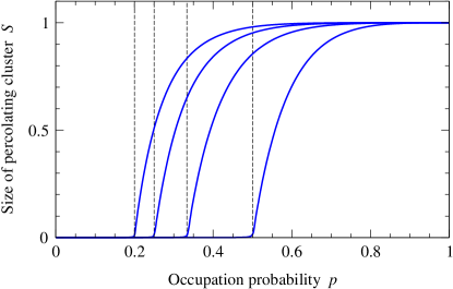
Figure 1: Size of the percolating cluster in numerical simulations of bond percolation on two-group networks of the type described in the text with $n=1\,000\,000$ nodes each. From left to right, the four curves have $(a,b)=(4,2)$, $(3,2)$, $(3,1)$, and $(2,1)$. The vertical dashed lines represent the theoretical predictions for the position of the percolation threshold, Eq. (7).

For our second example of solvable properties of equitable random graphs, we consider the spectral density of the adjacency matrix. Adjacency matrix spectra find uses in defining centrality measures, in algorithms for graph partitioning and community detection, in network visualization, and numerous other areas. The spectral density $\rho(z)=(1/n)\sum_{i}\delta(z-\lambda_{i})$ is the probability density of eigenvalues $\lambda_{i}$ and, as recently shown by Rogers et al. RCKT08 , it can be calculated on locally tree-like graphs using a message passing technique. In the formulation we use (which differs slightly from that of Rogers et al.) the messages are functions $g_{i\leftarrow j}(z)$ satisfying

$$g_{i\leftarrow j}(z)={1\over 1-z\sum_{k\in\mathscr{N}(j)\backslash i}\>g_{j\leftarrow k}(z)},$$ (8)

in terms of which the spectral density is

$$\rho(z)=-{z\over n\pi}\mathop{\mathrm{missing}}{Im}\sum_{i}{1\over z^{2}-\sum_{j\in\mathscr{N}(i)}\>g_{i\leftarrow j}(1/z^{2})}.$$ (9)

Again the crucial observation for equitable random graphs is that all edges between vertices in groups $\mu$ and $\nu$ have the same neighborhood out to arbitrary distances and hence that there exists a solution such that the message $g_{i\leftarrow j}(z)$ depends only on the groups to which $i$ and $j$ belong and not on the specific vertices. Equation (8) then simplifies to

$$g_{\mu\leftarrow\nu}(z)={1\over 1-z\sum_{\lambda}(m_{\nu\lambda}-\delta_{\lambda\mu})g_{\nu\leftarrow\lambda}(z)},$$ (10)

which reduces the problem of calculating the spectral density from one of solving $\mathrm{O}(m)$ equations to one of solving a fixed number $q^{2}$ even in an arbitrarily large system.

Taking once again the example of the two-group model with community structure discussed previously, there are in principle four different functions $g_{\mu\leftarrow\nu}(z)$, but because of symmetry between the groups all four are equal in this case, and Eq. (10) reduces to a single equation:

$$g(z)={1\over 1-(a+b-1)zg(z)}.$$ (11)

Solving the resulting quadratic and substituting the solution into (9), we find the spectral density to be

$$\rho(z)={(a+b)\over 2\pi}\,{\sqrt{4(a+b-1)-z^{2}}\over(a+b)^{2}-z^{2}},$$ (12)

which is a version of the Kesten–McKay distribution. Figure 2 shows an example spectrum for the case $a=3$, $b=1$ along with numerical results from direct diagonalization of the adjacency matrix for a computer-generated equitable random graph with the same parameters, and the agreement is excellent. Note that although the graph is extremely sparse in this case, the calculation still gives a correct result, by contrast with some other calculations of graph spectra, which fail in the sparse limit RB88 ; Kuhn08 .

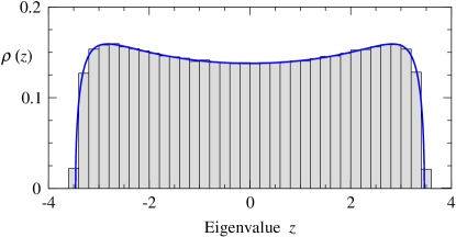
Figure 2: Spectrum of the two-group equitable random graph described in the text. The solid curve represents the analytic solution, Eq. (12), for the case $a=3$, $b=1$, while the histogram shows the results from the direct numerical diagonalization of a single computer-generated instance with $n=10\,000$ nodes and the same parameter values.

For our third example calculation with equitable random graphs we consider the evolution of a dynamical system on a network. In particular, we consider homogeneous systems, in which degrees of freedom on each vertex obey the same dynamics, and vertices are coupled along the edges of the network. Widely studied examples include coupled oscillators on networks and the dynamics of epidemic disease models such as the susceptible–infected–recovered (SIR) model.

Let us denote by $x_{i},y_{i},\ldots$ the degrees of freedom of a dynamical system on vertex $i$ of a network, let $\mathbf{r}_{i}=(x_{i},y_{i},\ldots)$, and let us write the dynamics in the standard form

$$\dot{\mathbf{r}}_{i}=\mathbf{f}(\mathbf{r}_{i})+\sum_{j}A_{ij}\mathbf{g}(\mathbf{r}_{i},\mathbf{r}_{j}),$$ (13)

where $A_{ij}$ is an element of the adjacency matrix. Here $\mathbf{f}(\mathbf{r})$ represents the intrinsic dynamics of the vertex (which is the same for every vertex), and $\mathbf{g}(\mathbf{r}_{i},\mathbf{r}_{j})$ represents the effect of vertex $j$ on vertex $i$. (Note that $\mathbf{g}$ is not necessarily symmetric in its arguments.) Systems with dynamics governed by second- or higher-order differential equations do not fit this form, but one can always reduce a set of second-order equations to twice as many first-order equations by introducing auxiliary variables, and similarly for higher orders.

As discussed by, for example, Golubitsky and Stewart GS06 , the size or complexity of dynamical systems on networks can in some cases be reduced significantly by exploiting network symmetries. Equitable random graphs do not typically possess significant symmetries, but nonetheless similar reductions are possible. We focus on the case where all vertices have the same initial condition (or, more generally, all vertices in each group of the random graph have the same initial condition). In this case, all vertices in each group will evolve in an identical fashion, because each, by definition, has the same intrinsic dynamics and feels the same influence from its neighbors. Thus our $n$ equations (13) immediately reduce to just $q$:

$$\dot{\mathbf{r}}_{\mu}=\mathbf{f}(\mathbf{r}_{\mu})+\sum_{\nu}m_{\mu\nu}\mathbf{g}(\mathbf{r}_{\mu},\mathbf{r}_{\nu}).$$ (14)

As an example, consider the SIR model of epidemic disease, whose state can be represented by $\mathbf{r}_{i}=(s_{i},x_{i},r_{i})$ on each vertex with $s_{i},x_{i},r_{i}$ denoting the probability that the vertex is, respectively, susceptible to, infected with, or recovered from the disease of interest at a given time, and $\mathbf{f}(\mathbf{r}_{i})=(0,-\gamma x_{i},\gamma x_{i})$, $\mathbf{g}(\mathbf{r}_{i},\mathbf{r}_{j})=(-\beta s_{i}x_{j},\beta s_{i}x_{j},0)$, where $\beta$ and $\gamma$ are constants representing the rate of infection and recovery per unit time respectively. For the equitable random graph we then have

$$\dot{s}_{\mu} =-\beta s_{\mu}\sum_{n}m_{\mu\nu}x_{\nu},$$ (15)

$$\dot{x}_{\mu} =\beta s_{\mu}\sum_{n}m_{\mu\nu}x_{\nu}-\gamma x_{\mu},$$ (16)

$$\dot{r}_{\mu} =\gamma x_{\mu},$$ (17)

in the approximation where all vertex states are considered independent. We can apply any of the standard techniques for nonlinear systems to this set of equations—finding fixed points, linear stability analysis, bifurcation analysis, or in some cases exact solutions. As an example, we can in this case make progress by eliminating $x_{\mu}$ between the first and third equations and integrating to get $s_{\mu}=\exp\bigl{[}-(\beta/\gamma)\sum_{\nu}m_{\mu\nu}r_{\nu}\bigr{]}$. At long times the disease always dies out, so that $x_{\mu}=0$, and combining this with the fact that $s_{\mu}+x_{\mu}+r_{\mu}=1$ we have

$$r_{\mu}=1-\exp\biggl{(}-{\beta\over\gamma}\sum_{\nu}m_{\mu\nu}r_{\nu}\biggr{)}$$ (18)

as $t\to\infty$. The solution to this equation tells us the number of recovered individuals at long times in each group, which is necessarily equal to the number of individuals who ever had the disease—in other words it tells us the size of the disease outbreak, group by group. We note that the equation always has a trivial solution at $r_{\mu}=0$ for all $\mu$, which corresponds to a situation in which there is no epidemic. It may or may not have a nontrivial solution, corresponding to the presence of an epidemic, depending on whether the rate of infection $\beta$ is large enough compared to the rate of recovery $\gamma$. Expanding the equation for small values of $r_{\mu}$ (i.e., close to the regime where there is no epidemic) and rearranging, we get $\sum_{\nu}m_{\mu\nu}r_{\nu}=(\gamma/\beta)r_{\mu}$, or $\mathbf{M}\mathbf{r}=(\gamma/\beta)\mathbf{r}$ in matrix notation. In other words, at the transition point $\mathbf{r}$ is the leading right eigenvector of the mixing matrix $\mathbf{M}$ and $\gamma/\beta$ is the corresponding eigenvalue. To put that another way, there will be an epidemic if, and only if, $\gamma/\beta$ is less than the leading eigenvalue of the mixing matrix. (A result reminiscent of this one is seen in epidemic behavior in stochastic block models—see BP02a .)

As an example, consider a network with two equally sized groups and mixing matrix

$$\mathbf{M}=\begin{pmatrix}4a&2a\\ 2a&a\\ \end{pmatrix}.$$ (19)

This model divides the network into a dense core (group 1) and a sparse periphery (group 2) with connections between them of intermediate density. Core–periphery structure of this kind is widely observed in real-world networks BE99 ; Holme05b ; RPFM14 . Since the leading eigenvalue of this mixing matrix is $5a$, we can immediately see that the epidemic threshold falls at $\gamma/\beta=5a$.

In summary, we have in this paper described a broad class of random graph models, which we call equitable random graphs, that is flexible enough to represent complex structure types such as community structure, core–periphery structure, and stratification, which have historically been of interest in the study of networked systems. At the same time these models can be solved for a range of nontrivial structural and dynamic properties, including percolation properties, graph spectra, and behavior of homogeneous dynamical systems on their vertices. This combination of flexibility and solvability gives equitable random graphs the potential to substantially enhance our understanding of the interplay between structure and function in networks.

The authors thank Brian Ball and Martin Golubitsky for useful conversations.

References

- (1) R. Solomonoff and A. Rapoport, Connectivity of random nets. Bulletin of Mathematical Biophysics 13, 107–117 (1951).
- (2) P. Erdős and A. Rényi, On random graphs. Publicationes Mathematicae 6, 290–297 (1959).
- (3) B. Bollobás, Random Graphs. Academic Press, New York, 2nd edition (2001).
- (4) M. Molloy and B. Reed, A critical point for random graphs with a given degree sequence. Random Structures and Algorithms 6, 161–179 (1995).
- (5) M. E. J. Newman, S. H. Strogatz, and D. J. Watts, Random graphs with arbitrary degree distributions and their applications. Phys. Rev. E 64, 026118 (2001).
- (6) P. W. Holland, K. B. Laskey, and S. Leinhardt, Stochastic blockmodels: Some first steps. Social Networks 5, 109–137 (1983).
- (7) B. Karrer and M. E. J. Newman, Stochastic blockmodels and community structure in networks. Phys. Rev. E 83, 016107 (2011).
- (8) S. Wasserman and K. Faust, Social Network Analysis. Cambridge University Press, Cambridge (1994).
- (9) M. Girvan and M. E. J. Newman, Community structure in social and biological networks. Proc. Natl. Acad. Sci. USA 99, 7821–7826 (2002).
- (10) S. Fortunato, Community detection in graphs. Phys. Rep. 486, 75–174 (2010).
- (11) R. Cohen, K. Erez, D. ben-Avraham, and S. Havlin, Resilience of the Internet to random breakdowns. Phys. Rev. Lett. 85, 4626–4628 (2000).
- (12) D. S. Callaway, M. E. J. Newman, S. H. Strogatz, and D. J. Watts, Network robustness and fragility: Percolation on random graphs. Phys. Rev. Lett. 85, 5468–5471 (2000).
- (13) P. Grassberger, On the critical behavior of the general epidemic process and dynamical percolation. Math. Biosci. 63, 157–172 (1983).
- (14) M. E. J. Newman, Spread of epidemic disease on networks. Phys. Rev. E 66, 016128 (2002).
- (15) B. Karrer, M. E. J. Newman, and L. Zdeborová, Percolation on sparse networks. Preprint arxiv:1405.0483 (2014).
- (16) T. Rogers, I. Pérez Castillo, R. Kühn, and K. Takeda, Cavity approach to the spectral density of sparse symmetric random matrices. Phys. Rev. E 78, 031116 (2008).
- (17) G. J. Rodgers and A. J. Bray, Density of states of a sparse random matrix. Phys. Rev. B 37, 3557–3562 (1988).
- (18) R. Kühn, Spectra of sparse random matrices. J. Phys. A 41, 295002 (2008).
- (19) M. Golubitsky and I. Stewart, Nonlinear dynamics of networks: The groupoid formalism. Bull. Amer. Math. Soc. 43, 305–364 (2006).
- (20) M. Boguñá and R. Pastor-Satorras, Epidemic spreading in correlated complex networks. Phys. Rev. E 66, 047104 (2002).
- (21) S. P. Borgatti and M. G. Everett, Models of core/periphery structures. Social Networks 21, 375–395 (1999).
- (22) P. Holme, Core-periphery organization of complex networks. Phys. Rev. E 72, 046111 (2005).
- (23) M. P. Rombach, M. A. Porter, J. H. Fowler, and P. J. Mucha, Core-periphery structure in networks. SIAM J. Appl. Math. 74, 167–190 (2014).