Schrödinger’s equation and “bike tracks” – a connection.

The purpose of this note is to demonstrate an equivalence between two classes of objects: the stationary Schrödinger equation on the one hand, and the “bicycle tracks” on the other. We begin with the description of the latter.

A (very) idealized model of a bicycle, shown in Figure 1, is a segment $RF$ of constant length which is allowed to move in the plane as follows: the path of the “front” $F$ is prescribed, while the velocity of the “rear” $R$ is constrained to the line $RF$: the “rear wheel” does not sideslip.

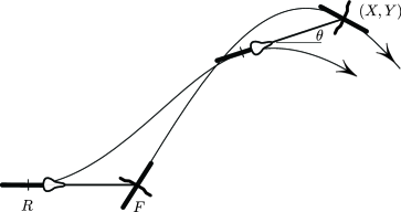
Figure 1: An idealized bike. In this example $F$ travels along an arc of a sine curve.

If $(X(t),Y(t))$ is a parametric representation of the motion of $F$ then the angle $\theta$ between $RF$ and the $x$–axis in the plane satisfies the differential equation

$$\dot{\theta}=\dot{Y}\cos\theta-\dot{X}\sin\theta,$$ (1)

expressing the fact that infinitesimal displacement of $R$ is aligned with the direction $e^{i\theta}$ of the segment.

Some examples of tracks are given in Figure 2.

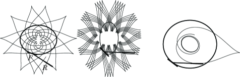
Figure 2: The path traced out by the rear wheel as the front wheel repeatedly traverses a closed curve.

A very brief history.

The idealized “bike” of Figure 1 has been studied since the second half of 19th century (see [5] and references therein), and up to the present time ([5, 11]). It was observed that the “bike” arises as an asymptotic limit of a system describing a particle in a rapidly oscillating potential; it is interesting that the nonholonomic “bike” is a singular limit of a holonomic system (the details can be found in [12], and in [10]).

Stationary Schrödinger’s equation

$$\ddot{x}+p(t)x=0$$ (2)

is a classical object of mathematical physics, arising in many settings in mathematics, physics and engineering. This system has been studied for nearly two centuries. Known also as Hill’s equation, it comes up in studying the spectrum of hydrogen atom, in celestial mechanics [18], in particle accelerators [23], in forced vibrations, in wave propagation, and in many more problems. Hill’s operator deforms isospectrally when its potential evolves under the Korteweg–de Vries(KdV) equation, thus providing an explanation of complete integrability of the latter [15], [8], [16]. The 1989 Nobel Prize in physics was awarded to W. Paul for his invention of an electromagnetic trap, now called the Paul trap, used to suspend charged particles. The mathematical substance of Paul’s discovery amounts to an observation on Hill’s equation, as expained in Paul’s Nobel lecture [17]. Incidentally, [9] contains a geometrical explanation, as an alternative to Paul’s analytical one, of why the trap works. Stability of the famous Kapitsa pendulum [1, 7] is also explained by the properties of Hill’s equation (Stephenson gave an experimental demonstration of stability of the so–called Kapitsa pendulum in 1908 [19], about half a century before Kapitsa’s paper). The long history of Hill’s equation is reflected in the rich body of classical literature of the 18th and 19th centuries on the eigenfunctions of special second order equations (polynomials of Lagrange, Laguerre, Chebyshev, Airy’s function, etc.), to the more recent work on inverse scattering and on geometry of “Arnold tongues” [20, 6, 2, 13, 21, 22, 14, 16, 4, 3], [13], [2], [21, 22].

1 The main result

Theorem 1

Let a Schrödinger potential $p(t)$ in (2) be given. We associate with $p$ the front wheel path $(X(t),Y(t))$ as follows: defining

$$\varphi(t)=t+\int_{0}^{t}p(s)\,ds,$$ (3)

we set

$$\left\{\begin{array}[]{l}X(t)=-\int_{0}^{t}(1-p(\tau))\sin\varphi(\tau)\;d\tau\\[3.0pt] Y(t)=\ \ \ \int_{0}^{t}(1-p(\tau))\cos\varphi(\tau)\;d\tau.\end{array}\right.$$ (4)

If the potential $p$ and the path $(X,Y)$ are thus related, then the two problems: the corresponding Schrödinger equation (2) and the bike problem (1) are equivalent in the sense that

$$\theta=2\arg(x+i\dot{x})+\varphi,$$ (5)

where $\varphi$ is given by (3).

Figure 3 shows paths corresponding to various potentials.

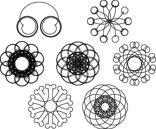
Figure 3: Front wheel paths representing different potentials. The top left corresponds to the solitary wave of the KdV. The remaining ones are generated by various trigonometric potentials. Alternatively, these paths are trajectories of the particle subject to the “magnetic” force (7) with different prescribed speeds $v=v(t)$.

1.1 A reformulation of the main result.

The track (4) can be thought of as the path of a particle subject to a strange magnetic–like force defined in the next paragraph.

A pseudo–magnetic force

Let $v=v(t)$ be a given function of time, and consider a point mass $m=1$ moving in the plane with speed $v$ and subject to normal acceleration due to the following magnetic–like force:

$${\bf F}={\bf a}_{\perp}=i\,(2-v){\bf v}$$ (6)

acting normal to the velocity ${\bf v}$. Note that the tangential velocity $v$ is prescribed (one can imagine a tangential force acting on the particle in addition to the normal force (6)), and that the normal acceleration is slaved to $v$. We allow $v$ to change sign, so that $v=\pm|{\bf v}|$; if $v$ changes sign, the particle reverses the direction of motion, as illustrated in Figure 4.

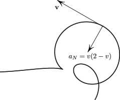
Figure 4: Trajectory of a particle subject to force (6) with $v$ prescribed. At the cusp $v$ changes sign.

The main result can now be reformulated as follows.

Theorem 2

Consider the Schrödinger equation (2) with potential $p(t)$. Define

$$v(t)=1-p(t),$$ (7)

and let $(X(t),Y(t))$ be a path of the “magnetic” particle defined in the preceding paragraph. Then the Schrödinger equation (2) and the bike problem (1) are equivalent, i.e. they transform into one another via the transformation

$$\theta=2\arg(x+i\dot{x})+\varphi,$$ (8)

where $\varphi=t+\int_{0}^{t}p(\tau)\,d\tau$.

2 Proofs.

Proof of Theorem 1. We begin by writing the Schrödiner equation (2) as a system

$$\left\{\begin{array}[]{l}\dot{x}=y\\[3.0pt] \dot{y}=-p(t)x\end{array}\right.$$ (9)

or in matrix form

$$\dot{z}=P(t)z,\ \ \hbox{with}\ \ P=\left(\begin{array}[]{cc}0&1\\ -p&0\end{array}\right).$$ (10)

The main point of the proof is to observe that Schrödiner equation (10) in a rotating frame becomes equivalent to the Ricatti equation for the bicycle. To make this precise, let

$$\psi=\psi(t)=-\frac{1}{2}\biggl{(}t+\int_{0}^{t}p(\tau)d\tau\biggl{)};$$ (11)

note that $\dot{x}\psi$ is half the curl of the vector field in (10), i.e. the average angular velocity of the vector field around the origin. Introduce the rotation through angle $\psi$:

$$R=R(t)=\left(\begin{array}[]{cc}\cos\psi&-\sin\psi\\ \sin\psi&\ \ \ \cos\psi\end{array}\right).$$ (12)

To rewrite the Schrödinger equation (10) in the rotating frame we introduce the new variable $w$ via

$$z=R_{\psi}w.$$ (13)

We obtain a new system equivalent to (10):

$$\dot{w}=(R^{-1}PR-R^{-1}\dot{R})w.$$ (14)

A computation confirms the expectation that coefficient matrix of this system should be symmetric (since we cancelled angular velocity) and traceless (since the transformation is area–preserving and since the original matrix was traceless):

$$R^{-1}PR-R^{-1}\dot{R}=\left(\begin{array}[]{cc}r&\ \ s\\ s&-r\end{array}\right),$$ (15)

where

$$\begin{array}[]{l}r=\frac{1}{2}(1-p)\sin 2\psi\\[3.0pt] s=\frac{1}{2}(1-p)\cos 2\psi.\end{array}$$ (16)

According to (13), we have

$$\arg(x+iy)=\arg w+\psi,$$ (17)

and we now show that $\theta=2\arg w$ satisfies the bicycle equation (1); this would complete the proof. Indeed, then (17) would become

$$\arg(x+iy)=\frac{1}{2}\theta+\psi,\ \ \hbox{or}\ \ \theta=2\arg z-2\psi,$$

which indeed coincides with (5) since $-2\psi=\varphi$ according to (11) and (3).

To derive the equation for $\arg w$ the we write our system (14)-(15) for $w$ explicitly:

$$\left\{\begin{array}[]{l}\dot{u}=ru+sv\\[3.0pt] \dot{v}=su-rv,\end{array}\right.$$ (18)

and let $\widehat{w}=\arg w=\arg(u+iv)$. Now

$$\frac{d}{dt}\widehat{w}=\frac{\dot{v}u-\dot{u}v}{u^{2}+v^{2}}\buildrel(\ref{eq:gl})\over{=}\frac{su^{2}-2ruv-sv^{2}}{u^{2}+v^{2}},$$

so that

$$\frac{d}{dt}\widehat{w}=s\cos^{2}\widehat{w}-2r\cos\widehat{w}\sin\widehat{w}-s\sin^{2}\widehat{w}$$

This can be rewritten in terms of double angle $2\widehat{w}$ as follows:

$$\frac{d}{dt}(2\widehat{w})=2s\cos 2\widehat{w}-2r\sin 2\widehat{w}.$$ (19)

This ODE is identical to the the bicycle equation:

$$\dot{\theta}=\dot{Y}\cos\theta-\dot{X}\sin\theta$$

provided we set

$$\dot{X}=2r,\ \ \dot{Y}=2s,$$

or, recalling the definition (16) of $r$ and $s$, provided

$$\begin{array}[]{l}\dot{X}=(1-p)\sin 2\psi=-(1-p)\sin\varphi,\\[3.0pt] \dot{Y}=(1-p)\cos 2\psi=\ \ (1-p)\cos\varphi.\end{array}$$ (20)

We conclude that $\theta=2\widehat{w}$ in the sense that both angles satisfy the same differential equation provided we define $X,\ Y$ by (20) or (4). This completes the proof. $\diamondsuit$

Proof of Theorem 2. Consider the motion $(X(t),Y(t))$ given by (4). The velocity of this motion

$$\left\{\begin{array}[]{l}\dot{X}=-(1-p(t))\sin\varphi\\[3.0pt] \dot{Y}=\ \ (1-p(t))\cos\varphi\end{array}\right.$$ (21)

The speed $v=1-p$ is in the direction $\varphi+\pi/2$ if $1-p>0$ and in the opposite direction if $1-p<0$. The angular velocity of this motion is

$$\omega=\dot{\varphi}=1+p,$$

and thus the normal acceleration

$$a_{\perp}=\omega v.$$

But

$$\omega=1+p\buildrel(\ref{eq:vp})\over{=}1+(1-v)=2-v,$$

so that $a_{\perp}=v(2-v)$. $\diamondsuit$

Acknowledgments. The author’s research was supported by an NSF grant DMS-0605878.

References

- [1] V.I. Arnold. On matrices depending on parameters. Russ. Math. Surv. 26, 1971.
- [2] V.I. Arnold. Remarks on the perturbation theory for problems of Mathieu type. Russ. Math. Surv. 38, 1983.
- [3] H. W. Broer and C.Simo. Resonance tongues in hill’s equations: A geometric approach. J. Diff. Equations 166 (2), pages 290–327, 2000.
- [4] H. W. Broer and M. Levi. Geometrical aspects of stability theory for hill’s equations. Arch. Rational Mech. Anal. 131, pages 225–240, 1995.
- [5] R. L. Foote. Geometry of the Prytz planimeter . Rep. Math. Phys. 42 no. 1-2, pages 249–271, 1998.
- [6] I.M. Gelfand and B.M. Levitan. On the determination of a differential equation from its spectral function. Amer. Math. Soc. Transl. 1(2), pages 253–304, 1955.
- [7] P.L. Kaptisa. Dynamical stability of a pendulum when its point of suspension vibrates. Collected Papers by P.L. Kapitsa, Volume II, Pergamon Press, London, pages 714–725, 1965.
- [8] P.D. Lax. Integrals of nonlinear equations of evolution and solitary waves. Comm. Pure Appl. Math. 21, page 467–490, 1968.
- [9] M. Levi. Stability of the inverted pendulum – a topological explanation. SIAM Review 30, pages 639–644, 1988.
- [10] M. Levi. Geometry and physics of averaging with applications. Physica D 132, pages 150–164, 1999.
- [11] M. Levi and S.Tabachnikov. On bicycle tire tracks geometry, menzin’s conjecture, and oscillation of unicycle tracks. Experimental Mathematics 18 2, pages 173–186, 2009.
- [12] M. Levi and W. Weckesser. Stabilization of the inverted linearized pendulum by vibration. SIAM Review Vol. 37 No. 2, pages 219–223, 1995.
- [13] D.M. Levy and J.B. Keller. Instability intervals of Hill’s equation. Comm. Pure Appl. Math., 16, 1963.
- [14] V. A. Marchenko. Sturm-Liouville operators and applications. Birkh user Verlag, Basel, 1986.
- [15] Gardner C.S., Miura R. M. and Kruskal M. D. Korteweg-devries equation and generalizations. II. Existence of conservation laws and constants of motion. Journal of Math. Phys., 9, pages 1204–1209, 1968.
- [16] S.P. Novikov. A periodic problem for the Korteweg-de Vries equation. I. Functional Anal. Appl. 8(3), pages 236–246, 1974.
- [17] W. Paul. Electromagnetic traps for charged and neutral particles. Revs. Mod. Phys. 62, pages 531–540, 1990.
- [18] C.L. Siegel and J.K. Moser. Lectures on Celestial Mechanics. Grundlehren der mathematischen Wissenschaften, 87. Springer, 1971.
- [19] A. Stephenson. On a new type of dynamical stability. Manchester Memoirs, 52, pages 1–10, 1908.
- [20] B. van der Pol and M.J.O. Strutt. On the stability of the solutions of Mathieu’s equation. The London, Edinburgh and Dublin Phil. Mag. 7th series 5, 1928.
- [21] M.I. Weinstein and J.B. Keller. Hill’s equation with a large potential. SIAM J. Appl. Math. 45, pages 200–214, 1985.
- [22] M.I. Weinstein and J.B. Keller. Asymptotic behavior of stability regions for Hill’s equation. SIAM J. Appl. Math. 47, 1987.
- [23] H. Wiedemann. Particle Accelerator Physics. Springer-Verlag Berlin Heidelberg, 2007.