Solitons with nested structure over finite fields

Abstract

We propose a solitonic dynamical system over finite fields that may be regarded as an analogue of the box-ball systems. The one-soliton solutions of the system, which have nested structures similar to fractals, are also proved. The solitonic system in this paper is described by polynomials, which seems to be novel. Furthermore, in spite of such complex internal structures, numerical simulations exhibit stable propagations before and after collisions among multiple solitons with preserving their patterns.

1 Introduction

The box-ball system (BBS)[15] has been extensively studied as digitalized integrable systems. The properties of the BBS such as the relation to the discrete KP (or KdV) equation and its conserved quantities etc. has been well understood through the ultradiscretization[17]. From the ultradiscretized system, we may frequently obtain systems such as cellular automata over integers by limiting the parameters and initial values to integers. This limitation is, however, not necessarily required for the equation itself. The ultradiscretized equations may be essentially regarded as the systems over real or rational numbers[7]. In many cases of the integrable ultradiscrete systems that has been hitherto known, their integrability has a close relationship with that of the corresponding discrete system before ultradiscretization; therefore, the integrability of the ultradiscrete system may be considered to be guaranteed by that of the corresponding discrete system. This property is one of remarkable merits of ultradiscretization for proving the integrability of the given system as a matter of course. However, on the other hand, intrinsic qualities of ultradiscretized system seems to be hidden behind the outstanding ultradiscretized correspondence. In this paper, we consider a solitonic dynamical system in which the dependent variables are over finite fields. By investigating integrable dynamical systems over finite fields without such an a priori relationship, novel insights about integrability itself may be expected.

Below are the examples of integrable systems over finite fields. In [3], filter type cellular automata (CA) are constructed from the Schrödinger discrete spectral problem[4] that have infinitely many conserved quantities. In [2], integrable CA over cyclic group is obtained from the discrete sine-Gordon equation (Hirota equation) as Möbius transformation. These two systems possess the Lax representation. The algebro-geometric method for constructing solutions of the discrete KP equation and the discrete Toda equation over finite fields is shown in [1, 5], whose $\tau$ function in the bilinear form has $N$-soliton solutions. Three examples above do not seem to have solitonically propagating waves. In [9], the discrete integrable system over the rational function field with indeterminate over ${\mathbb{F}}_{q}$ is obtained from the generalized discrete KdV equation. The $p$-adic valuations of variables for the discrete KdV equation are also discussed in [8], which is considered as an analogue of ultradiscretization. As an application of integrable systems over finite fields, the relationship between the dynamics of Toda molecule over finite fields and the BCH-Goppa decoding is discussed in [12].

In this paper, we construct a formal analogue of the BBS over finite fields from the point of view of ultradiscrete bilinear form. This paper is organized as follows: In section 2, we give a brief introduction of the BBS, which is compared with the ffBBS we propose in section 3. In section 4, the ffBBS with $p=3$ is shown together with numerical simulations that exhibit stable propagations of solitons over finite field ${\mathbb{F}}_{3}$. Then in section 5, the exact one-soliton solutions, which have a nested structure similar to fractals, are proved. The last section 6 is devoted to the conclusion and summary obtained in this paper.

2 Box-Ball System (BBS)

In this paper we propose the system that is an analogue of the BBS and investigate its properties. For the purpose of comparison, we summarize several matters relating to the BBS below [15, 17, 16].

The BBS in the case that the capacity of each box is constant $L$ is shown as follows:

$$u^{t+1}_{n}:=\min\left\{L-u^{t}_{n},\sum^{n-1}_{i=-\infty}\left(u^{t}_{i}-u^{t+1}_{i}\right)\right\}+\max(0,-L),$$ (1)

where $u^{t}_{n}$ is the dependent variable that is interpreted as the number of balls in the box at time $t$ and position $n$. By the transformation between the dependent variables

$$u^{t}_{n}=s^{t}_{n}-s^{t}_{n-1},\qquad s^{t}_{n}=g^{t-1}_{n}-g^{t}_{n},$$ (2)

we obtain the ultradiscrete bilinear form under appropriate boundary conditions as follows:

$$s^{t+1}_{n+1}-s^{t}_{n}-\max(0,-L) = \min\left(0,L-s^{t}_{n+1}+s^{t+1}_{n}\right),$$ (3)

$$g^{t+1}_{n+1}+g^{t-1}_{n}+\max(0,-L) = \max\left(g^{t}_{n+1}+g^{t}_{n},g^{t-1}_{n+1}+g^{t+1}_{n}-L\right).$$ (4)

Because the parameter $L$ is usually interpreted as the maximum number of balls that are stuffed into each box, $L$ is assumed to be positive ($L>0$) for obtaining meaningful equations as the dynamics of ball moving. Ordinarily, the term $\max(0,-L)$ is eliminated as a matter of course. However, the term $\max(0,-L)$ is left in (1)–(4) as it is for the next section on purpose. Furthermore by the transformation of variables $c^{t}_{n}:=s^{t}_{n-1}-s^{t+1}_{n-1}$, we obtain

$$u^{t+1}_{n} = \min\left(L-u^{t}_{n},c^{t}_{n}\right)+\max(0,-L)$$ (5)

$$= c^{t}_{n}-\max\left(u^{t}_{n}+c^{t}_{n}-L,0\right)+\max(0,-L),$$

$$c^{t}_{n+1} = u^{t}_{n}+c^{t}_{n}-u^{t+1}_{n}$$ (6)

$$= u^{t}_{n}+\max\left(u^{t}_{n}+c^{t}_{n}-L,0\right)-\max(0,-L)$$

from (3), which stands for the combinatorial $R$[6]. This dependent variable $\left\{c^{t}_{n}\right\}$ is called a carrier[14]. The BBS we have shown here is the case of the carrier without limit (the capacity of the carrier is $\infty$). The time evolution of the BBS from $t$ to $t+1$ with $L=1$ is interpreted as the interaction between this carrier and the balls:

1. The carrier repeats (ii) and (iii) through all boxes from left to right.

2. If a ball is in the box, the carrier picks up the ball.

3. If the box is empty and the carrier contains at least one ball, the carrier drops one ball into the box.

Figure 1 shows the examples of time evolution of the BBS.

Figure 1: A example of time evolution of BBS by (1) with $L=1$.

3 Soliton equation over finite fields (ffBBS)

The BBS we have observed in the previous section is the well-studied system, and its important properties such as solutions, conserved quantities etc. are well-known. It is genuine integrable soliton systems with the $\left\{0,1,\ldots,L\right\}$-valued dependent variables $\left\{u^{t}_{n}\right\}$. However, even in the case $L=1$, (1)–(4) are equations over not binary but integer (or real number), because the state of the carrier $c^{t}_{n}$, i.e. the number of balls contained in the carrier, is specified by an integer (or real number). One of our motivation stated in the introduction is to obtain an integrable system which does not have relation to ultradiscretization. In the following section, we define a system of which all dependent variables are the elements in finite set, which also have good algebraic structures, namely the finite fields.

3.1 A system similar to BBS

In this paper, we consider an analogue of the BBS over finite fields, based on the expressions (1)–(4). However, for example, trials for regarding (1) as an equation over finite fields do not apparently go well. Because the finite fields are not totally ordered sets and there is no definitions of magnitude relationship, we may not apply the minimum function $\min(\cdot,\cdot)$ in (1) as it is. To that end, we observe the algebraic operation needed for the transformations among equations (1)–(4). Then we find that, in addition to the four arithmetic operations of finite fields, the distributive law for the maximum function as binary operation, that is,

$$\max(x,y)+z=\max(x+z,y+z)$$ (7)

are used ($x,y,z\in{\mathbb{R}}$). Note that the addition is ‘$\max$’ and the multiplication ‘$+$’ in max-plus algebra, and that $\min(\cdot,\cdot)$ is defined by $\max(\cdot,\cdot)$ as $\min(x,y):=-\max(-x,-y)$. In other words, the operation needed for $\max$ in the transformations (1)–(4) is only the distributive law for $\max$ and $+$, and such a property that $\max$ is the function that returns the maximum value is not required.

Accordingly, we make a trial of replacing the binary operation $\max:{\mathbb{R}}\times{\mathbb{R}}\to{\mathbb{R}}$ by a function $M:{\mathbb{F}}_{q}\times{\mathbb{F}}_{q}\to{\mathbb{F}}_{q}$ with the following properties (8), (9), and (10);

$$M(0,0)=0,$$ (8)

$$M(a,b)=M(b,a) : \mbox{commutative law},$$ (9)

$$M(a,b)+c=M(a+c,b+c)\quad : \mbox{distributive law},$$ (10)

where $a,b,c\in{\mathbb{F}}_{q}$ and $q:=p^{m}$. These properties yield

$$M(a,b)-M(-a,-b)=a+b,$$

which may be regarded as an analogue of the formula of $\max$

$$\max(x,y)-\max(-x,-y)=\max(x,y)+\min(x,y)=x+y.$$

Namely, $\min(\cdot,\cdot)$ in (1) is also replaced by means of this function $M$ as above.

Proposition 1

In the case $p=2$, there does not exist a function $M$ that satisfies (8), (9), and (10).

Proof

$M(0,1)=M(-1,0)+1=M(1,0)+1=M(0,1)+1$. $\Box$

Proposition 2

If the associative law

$$M(a,M(b,c))=M(M(a,b),c)$$ (11)

is also required in addition with (8), (9), and (10), there does not exist a binary operation $M$ over ${{\mathbb{F}}_{q}}^{2}$ that satisfies these four properties.

Proof

We will prove by contradiction with the assumption that there exists $M$ that satisfies (8), (9), (10), and (11). In this proof, define $f(x):=M(0,x)$ and ${\cal I}:=\left\{f(x)\left|x\in{\mathbb{F}}_{q}\right.\right\}\subseteq{\mathbb{F}}_{q}$, which is the image of the map $f$. Then, $f(0)=0$ immediately follows from (8), and $\forall x\in{\mathbb{F}}_{q},f(x)=f(-x)+x$ from $M(x,0)=M(0,-x)+x$, and $\forall x\in{\mathbb{F}}_{q},f(f(x))=f(x)$ from $M(M(x,0),0)=M(x,M(0,0))=M(x,0)$. That is, for all $y\in{\cal I}$, $f(y)=y$ and therefore $f(-y)=f(y)-y=0$. Note that $0\in{\cal I}$ from $f(0)=0$. For all $y,z\in{\cal I}$, we also obtain the following:

$$f(y+z) = f(f(y)+z)$$

$$= M(M(y,0)+z,0)$$

$$= M(M(y,0),-z)+z$$

$$= M(y,M(0,-z))+z$$

$$= M(0,M(0,-z)-y)+y+z$$

$$= f(f(-z)-y)+y+z$$

$$= f(-y)+y+z$$

$$= y+z.$$

If ${\cal I}=\left\{0\right\}$, then since ${\cal I}$ is the image of the map, the function values are always zero $f(x)=0$ and $f(-x)=0$ even for non-zero $x\in{\mathbb{F}}_{q}^{\times}$. This contradicts as $x=f(x)-f(-x)=0$. Thus, the image ${\cal I}$ contains at least one non-zero element $\exists x_{*}(\neq 0)\in{\cal I}$ and is at least one or higher-dimensional vector space with the non-zero element $x_{*}$.

For this element $x_{*}\in{\cal I}$, we have $f(-x_{*})=0$ whereas $f(-x_{*})=f((p-1)x_{*})=(p-1)f(x_{*})=-f(x_{*})=-x_{*}$, where $p$ is the characteristic of ${\mathbb{F}}_{q}$ ($q=p^{m}$). This contradicts $x_{*}\neq 0$, so the proof is complete. $\Box$

Let $\nu$ be $(p-1)/2\in{\mathbb{Z}}$ because $p$ is an odd prime from proposition 1. For simplicity, we restrict ourselves to the prime field case ($m=1$) hereafter. The map $M$ that satisfies (8), (9), and (10) is uniquely parametrized by only the values of $M(0,j)\ (j=1,2,\ldots,\nu)$, because $M(0,-j)$ is obtained from the relation $M(0,-j)=M(0,j)-j$ by noticing $-j=\nu+1,\nu+2,\ldots,2\nu=p-1$. Hence, the $M$ may be expressed by $\nu$-tuple of $e_{j}\left(\equiv M(0,j)\right)$ as

$$M(0,a)\equiv M^{(e_{1},e_{2},\ldots,e_{\nu})}(0,a):=\sum^{\nu}_{j=1}(\delta_{a,j}e_{j}+\delta_{a,-j}(e_{j}-j)),$$

where $\delta$ is the Kronecker delta,

$$\delta_{b+c,c} := -(b+1)(b+2)\cdots(b+p-1)$$

$$= \left\{\begin{array}[]{ll}1&(b=0)\\ 0&\mbox{otherwise}\end{array}\right.,\ \forall b,c\in{\mathbb{F}}_{p},$$

which is equivalent to Wilson’s Theorem; $(p-1)!+1\equiv 0\ (\mbox{mod}\ p)$. Note that $M(0,a)$ is the polynomial, which is parametrized by $(e_{1},e_{2},\ldots,e_{\nu})\in{{\mathbb{F}}_{p}}^{\nu}$. We will abbreviate $M^{(e_{1},e_{2},\ldots,e_{\nu})}$ to $M$ hereafter.

By means of this polynomial function $M$, we propose the following bilinear equation as the starting point of our system over finite fields (cf. (4)).

$$G^{t+1}_{n+1}+G^{t-1}_{n}+M(0,-L)=M\left(G^{t}_{n+1}+G^{t}_{n},G^{t-1}_{n+1}+G^{t+1}_{n}-L\right).$$ (13)

We will refer to (13) as the box-ball system over finite fields (ffBBS). Introducing the dependent variables similar to (2) as

$$U^{t}_{n}=S^{t}_{n}-S^{t}_{n-1},\qquad S^{t}_{n}=G^{t-1}_{n}-G^{t}_{n},$$ (14)

we obtain

$$U^{t+1}_{n}=-M\left(-L+U^{t}_{n},-\sum^{n-1}_{i=-\infty}\left(U^{t}_{i}-U^{t+1}_{i}\right)\right)+M(0,-L),$$ (15)

$$S^{t+1}_{n+1}-S^{t}_{n}-M\left(0,-L\right)=-M\left(0,-L+S^{t}_{n+1}-S^{t+1}_{n}\right),$$ (16)

which are the analogues of (1)–(4). The dependent variables $G^{t}_{n}$, $S^{t}_{n}$, $U^{t}_{n}$, and the parameter $L$ are elements in ${\mathbb{F}}_{p}$, and the independent variables $n$ and $t$ are those in ${\mathbb{Z}}$. The carrier interpretation (5) and (6) also holds by replacing $\max$ by $M$. This ffBBS is apparently reversible with respect to $t\to-t$ and $n\to-n$, which follows from the so-called unitarity condition of $R$ matrix. Note that the indeterminate such as division by zero does not appear for all initial values because the evolution in this system is described by polynomials. This is a remarkable feature of (13)-(16) compared with the preceding studies of dynamical systems over finite fields stated in the introduction.

3.2 zero-soliton solution

In BBS (4), it is well known that $g^{t}_{n}=\mbox{const.}$ gives the zero-soliton solution and yields $u^{t}_{n}=0$, i.e., the state without balls. From the above correspondence, it is clear that $G^{t}_{n}=\mbox{const.}$ gives the zero-soliton solution and yields $U^{t}_{n}=0$ for ffBBS (15). Thus, we may easily obtain the zero-soliton solution due to the formal analogue. In the next section, we will observe the typical solutions of the ffBBS.

4 Simplest case: $p=3$

Hereafter we limit ourselves to the prime field ${\mathbb{F}}_{3}$, which is the simplest case because $p$ should be odd from proposition 1. In this case $p=3$, the function $M$ is determined by only one parameter $e_{1}\in{\mathbb{F}}_{3}$ due to $\nu=1$ as

$$M^{(e_{1})}(a,b):=(e_{1}+1)(a^{2}+ab+b^{2})+2(a+b).$$ (17)

For $e_{1}=2$, the function $M^{(2)}$ become first-degree polynomial and determine only trivial systems. The relation $M^{(1)}(a,b)=2^{-1}M^{(0)}(2a,2b)$ implies that $M^{(1)}$ and $M^{(0)}$ are isomorphic ($2^{-1}\equiv 2\bmod 3$). For this reason, we hereafter consider only $M^{(1)}(a,b)=2(a^{2}+ab+b^{2}+a+b)$ as $M$. The following is then satisfied.

Fact 3

$M^{(1)}(0,0)=0,M^{(1)}(0,1)=1,M^{(1)}(0,2)=0$.

Let $L$ be fixed to one so that $M(0,-L)=0$ for simplicity. In this paper we will obtain the one-soliton solutions only for this particular ${\mathbb{F}}_{3}$ with $e_{1}=1$ and $L=1$. The general ${\mathbb{F}}_{q}$ cases are subjects for future analysis, though our numerical experiments show abundant solitonic patterns.

4.1 One-soliton solutions with integer velocities

The stable solitary wave that is separated by sufficient ‘0’s is called soliton in this paper. An example of three kinds of solitons is shown in figure 2(a) ($p=3,e_{1}=1,L=1$). First, the pattern with ‘0’s (e.g. white part in lower left area) is zero-soliton solutions. On this background, the solitons ‘11’, ‘1’, ‘2’, ‘2’ are moving to the right with the velocity 2, 1, 0, 0, respectively. Stable propagations are observed before and after collisions with some phase shifts, which are similar to the BBS solutions in figure 1.

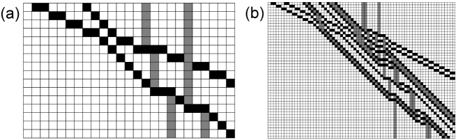
Figure 2: Examples of time evolution of ffBBS by (15) with $p=3,e_{1}=1,L=1$  (White: 0, Black: 1, Gray: 2). As initial values, solitons which have velocities (a) 2, 1, 0, 0 (b) 2, 2, 1, 1, 1, 0, 0 are given at uppermost row.

We elucidate the travelling waves by assuming $G(\xi)\equiv G^{t}_{n}$, $\xi:=Kn-\Omega t$. Substituting these into (13) and (16), we obtain

$$G(\xi+K-\Omega)+G(\xi+\Omega) =$$ (18)

$$M\left(G(\xi+K)+G(\xi),G(\xi+K+\Omega)+G(\xi-\Omega)-1\right),$$

$$S(\xi+K-\Omega)-S(\xi)=-M\left(0,S(\xi+K)-S(\xi-\Omega)-1\right).$$ (19)

Choosing $\Omega=0$ yields the solution with velocity zero $S(\xi+K)-S(\xi)=0\mbox{ or }2$ from (19); that is, $U^{t}_{n+1}=0\mbox{ or }2$, since $U^{t}_{n+1}=S(\xi+K)-S(\xi)$. Thus initial states that consist of only ‘0’s and ‘2’s give the patterns that do not move.

Next, we consider travelling waves with velocity one. Applying $\Omega=K$ to (18) with the distributive law (10) yields

$$M\left(0,G(\xi+2K)-G(\xi+K)-G(\xi)+G(\xi-K)-1\right)=0.$$ (20)

Substituting

$$U^{t}_{n} = G^{t-1}_{n}-G^{t}_{n}-G^{t-1}_{n-1}+G^{t}_{n-1}$$

$$= G(\xi+\Omega)-G(\xi)-G(\xi-K+\Omega)+G(\xi-K)$$

$$= G(\xi+K)-2G(\xi)+G(\xi-K)$$

into (20), we obtain the implicit equation $M\left(0,U^{t}_{n+1}+U^{t}_{n}-1\right)=0.$ The solution is $U^{t}_{n+1}+U^{t}_{n}=0\mbox{ or }1$; that is,

$$(U^{t}_{n},U^{t}_{n+1})\in\left\{(0,0),(0,1),(1,0),(1,2),(2,1),(2,2)\right\}$$ (21)

for all $t$ and $n\in{\mathbb{Z}}$. Since the zero-soliton solution consists of only ‘0’s and the combination $(0,2)$ is not contained in the above set, we may find that the left end of the pattern of the travelling wave with velocity one starts from ‘1’. Likewise, we may find that the right end of the pattern ends with ‘1’ since $(2,0)$ is not allowed. Shifting $n$ and combining the adjacent $U^{t}_{n}$ and $U^{t}_{n+1}$ in (21), we obtain the one-soliton patterns ‘$\cdots 010\cdots$’ in the case without ‘$2$’, and ‘$\cdots 012(12+2)^{*}10\cdots$’ (regular expression) otherwise. (e.g. ‘010’, ‘01210’, ‘012210’, ‘0121210’, ‘0122210’, $\dots$ ).

Finally, we consider travelling waves with velocity two. Applying $\Omega=2K$ to (18) yields

$$G(\xi-K)+G(\xi+2K) =$$

$$M\left(G(\xi+K)+G(\xi),G(\xi+3K)+G(\xi-2K)-1\right).$$

Substituting $U^{t}_{n}=G(\xi+2K)-G(\xi+K)-G(\xi)+G(\xi-K)$ into the above equation, we obtain $U^{t}_{n}=M\left(0,U^{t}_{n+1}+U^{t}_{n}+U^{t}_{n-1}-1\right)$, which have the solutions

$$(U^{t}_{n-1},U^{t}_{n},U^{t}_{n+1})\in\left\{(0,0,0),(0,0,1),(0,1,1),(1,0,0),(1,1,0)\right\}$$

for all $t$ and $n\in{\mathbb{Z}}$. Combining these adjacent relations, we obtain only ‘$\cdots$001100$\cdots$’.

Figure 2(b) shows the examples of solitons that we have proved here. Note that we regard the pattern with only 0’s (white cells) as the zero-soliton solution rather than the one with velocity zero. Each shape of the solitons is preserved as well in spite of collisions. We summarize the above solutions as follows:

Theorem 4 (one-soliton solutions with integer velocities)

• The patterns with velocity zero consist of only ‘$2$’.

• The patterns with velocity one are, ‘$010$’ and ‘$012(12+2)^{*}10$’ (regular expression). Namely, there exist infinite kinds of patterns with velocity one that does not contain ‘$0$’ inside them (‘$010$’, ‘$01210$’, ‘$012210$’, ‘$0121210$’, ‘$0122210$’, $\dots$ ).

• The pattern with velocity two is only ‘$11$’.

Besides the soliton solutions with integer speed 0, 1, and 2 shown in theorem 4, there exist travelling waves with $\Omega=K+1=2^{h+1}$ for all $h\in{\mathbb{Z}}_{>0}$. These solutions are shown in theorem 5, which contain the pattern ‘$12^{h}0^{h}1$’ at a certain time. In the case $h=0$, this pattern coincides with the soliton ‘11’ in theorem 4.

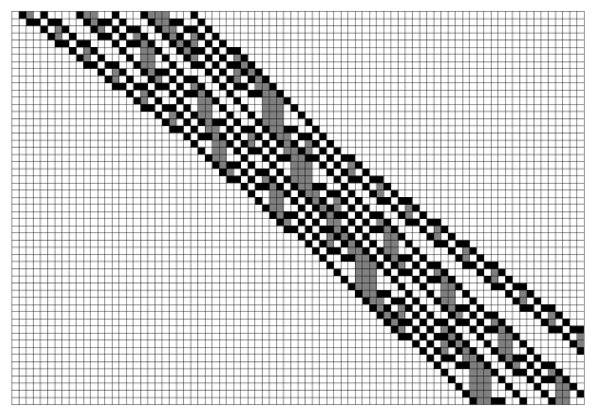
Figure 3: An example of time evolution by (15) with $p=3$, $e_{1}=1$, and $L=1$  (White: 0, Black: 1, Gray: 2). As initial values, three solitons that have velocity 4/3, 8/7, 16/15 respectively described in theorem 5 are given at uppermost row. Despite complex collisions, three solitons conserve their patterns.

Figure 3 shows an example of solitonic interactions between these travelling waves, in which the patterns ‘1201’, ‘122001’, ‘12220001’ are given respectively as initial values. The dispersion relation $\Omega=2^{h+1}$, $K=2^{h+1}-1$ leads to the fractional velocities $2^{h+1}/(2^{h+1}-1)$; that is, the same pattern appears again at $2^{h+1}-1$ time later at the position shifted $2^{h+1}$. Note that (15) is reversible.

It is not proved whether there exist one-soliton solutions besides those shown in this section. However, our numerical experiments show that the above patterns are all.

5 One-soliton solutions with fractional velocities

In this section, we prove that there exist the travelling waves with the fractional velocities $2^{h+1}/(2^{h+1}-1)$ for all $h\in{\mathbb{Z}}_{>0}$.

5.1 Definitions

Let $h$ be a positive integer and $\Omega=K+1=2^{h+1}$ through this section. Suppose the integer sequences that are recursively defined as follows:

• $I^{(h)}_{h}:=(2^{h+1}-1)$.

• For $1\leq i\leq h$, the sequence $I^{(h)}_{i-1}$ is defined by the following two steps:

  1. copy $I^{(h)}_{i}$.

  2. simultaneously replace all $\underline{2^{i+1}-1}$ with $\underline{(1,2^{i}-1,2^{i}-1)}$.

Note that $I^{(h)}_{i}$ ($1\leq i\leq h$) consists of $1$’s and $(2^{i+1}-1)$’s, and $1$’s are never replaced in the step (ii). Though we represent the sequences with parentheses to express the tree structure accompanied by the replacements of integers, the parentheses are ignored as for the integer sequences (cf. figure 5). For specification of each element in $I^{(h)}_{i}$, we define the numbering

$$I^{(h)}_{i}=:(I^{(h)}_{i}(0),I^{(h)}_{i}(1),\ldots,I^{(h)}_{i}(2^{h-i+1}-2)),$$

where the length of the integer sequence $I^{(h)}_{i}$ is $2^{h-i+1}-1$. The summation of the elements in this sequence $I^{(h)}_{i}$ is

$$\sum_{k=0}^{2^{h-i+1}-2}I^{(h)}_{i}(k)=2^{h+1}-1=K\quad(0\leq i\leq h),$$ (22)

and does not depend on $i$ because the two underlined parts above have the same summation $2^{i+1}-1$.

We define the palindromic sequence $I^{(h)}$ by aligning $I^{(h)}_{i}$ as follows:

$$I^{(h)} := (I^{(h)}_{h},I^{(h)}_{h-1},\ldots,I^{(h)}_{1},\overbrace{1,1,\ldots,1}^{2^{h+1}+h-1},I^{(h)R}_{1},I^{(h)R}_{2},\ldots,I^{(h)R}_{h})$$ (23)

$$= (I^{(h)}_{h},I^{(h)}_{h-1},\ldots,I^{(h)}_{1},I^{(h)}_{0},\overbrace{1,1,\ldots,1}^{h},I^{(h)R}_{1},I^{(h)R}_{2},\ldots,I^{(h)R}_{h}),$$ (24)

where $X^{R}$ is the reverse string of $X$ (each of symbol here is integer). Simple calculations show that the length of the sequence $I^{(h)}$ is $r:=3\cdot 2^{h+1}-(h+5)$, and the summation is $(2h+1)2^{h+1}-(h+1)$. Note that (24) follows from the fact that $I^{(h)}_{0}$ consists of $(2^{h+1}-1)$ 1’s.

Furthermore let us define the sequential numbering of the elements in $I^{(h)}$ with the length $r$ as $(b_{0},b_{1},\ldots,b_{r-1}):=I^{(h)}$. In other words, for $0\leq\forall l\leq 2^{h+2}-(h+4)$, there exists a unique $i$ such that $2^{h-i+1}-(h-i+2)\leq l<2^{h-i+2}-(h-i+3)$, and we have

$$0\leq i\leq h,\ b_{l}=I^{(h)}_{i}(l-2^{h-i+1}+(h-i+2)).$$ (25)

For $2^{h+2}-(h+3)\leq l\leq r-1$, $b_{l}$ may be palindromically defined by $b_{r-l-1}$. We also define the set $J:=\left\{a_{0},a_{1},\ldots,a_{r}\right\}$ by the recurrence equation $a_{l+1}=a_{l}+b_{l},a_{0}=0$. Namely, $a_{l}$ is the summation of $b_{l}$, and $a_{r}=(2h+1)2^{h+1}-(h+1)$ is the maximal element in $J$. Suppose the function $S(\xi):=\displaystyle\sum_{\mu\in J}\theta(\xi-\mu)\bmod 3\in{\mathbb{F}}_{3}$, where $\theta(\xi)$ be the unit step function that is defined over integer $\xi$ as $\displaystyle\theta(\xi)=\left\{\begin{array}[]{ll}1&(0\leq\xi)\\ 0&\mbox{otherwise}\end{array}\right.$. We then obtain the following theorem.

Theorem 5

Let $h$ be an positive integer, and $\Omega=K+1=2^{h+1}$. Then, $S(\xi)$ defined above is the solution of (19). The corresponding travelling wave solution $\left\{U^{t}_{n}\right\}$ of (15) contains the pattern ‘$12^{h}0^{h}1$’ at a certain time, and have fractional velocity $\Omega/K=2^{h+1}/(2^{h+1}-1)$.

Example 1 (The case $h=3$)

Suppose $h=3$ as an example, then we have $K=15,\Omega=16,r=40$. The initial sequence is defined as $I^{(3)}_{3}=(15)$ with the length one. $I^{(3)}_{2}$ is obtained by replacing the value 15 in $I^{(3)}_{3}$ with $(1,7,7)$, i.e., $I^{(3)}_{2}=((1,7,7))$. Furthermore, replacing each 7’s in $I^{(3)}_{2}$ with $(1,3,3)$ respectively yields $I^{(3)}_{1}=((1,(1,3,3),(1,3,3)))$. Combining these sequences, we obtain

$$I^{(3)} = ((15),((1,7,7)),((1,(1,3,3),(1,3,3))),$$

$$\qquad\overbrace{1,1,1,1,1,1,1,1,1,1,1,1,1,1,1,1,1,1}^{18},$$

$$\qquad(((3,3,1),(3,3,1),1)),((7,7,1)),(15)),$$

and $b_{0}=15,b_{1}=1,b_{2}=7,b_{3}=7,b_{4}=1,\ldots,b_{38}=1,b_{39}=15$, and $a_{0}=0,a_{1}=15,a_{2}=16,a_{3}=23,a_{4}=30,a_{5}=31,\ldots,a_{39}=93,a_{40}=108$ sequentially from the left. Substituting $K$ and $\Omega$ into (19) yields

$$S(\xi)-S(\xi-1)=M\left(0,S(\xi+15)-S(\xi-16)-1\right).$$

Let us suppose $\xi=15$ for example, then this equation holds as follows. The left-hand side of the above equation equals one due to $a_{1}=15$, while the right-hand side results in $M(0,5-1)=M(0,1)=1$ because the elements in $J$ that satisfy $0\leq a_{i}\leq 30$ are the ones with $0\leq i\leq 4$ and accordingly the number of them is five.

The rewriting rule in the above definition of $I^{(h)}_{i-1}$ is simultaneously applied. Therefore this grammar is a kind of L-system (Lindenmayer system)[10]. Consider the grammar $G^{\prime}:=\langle\Sigma^{\prime},\omega,P\rangle$, where the alphabet $\Sigma^{\prime}=\left\{{\tt A},{\tt B}\right\}$, the start symbol $\omega={\tt B}\in\Sigma^{\prime}$, the production rule $P=\left\{{\tt A}\to{\tt A},{\tt B}\to{\tt A}{\tt B}{\tt B}\right\}$. Replacing the derived strings $\left\{{\tt B},{\tt A}{\tt B}{\tt B},{\tt A}{\tt A}{\tt B}{\tt B}{\tt A}{\tt B}{\tt B},\ldots\right\}$ with ${\tt A}\mapsto 1,{\tt B}\mapsto 2^{i}-1$ then yields $I^{(\cdot)}_{i-1}$. Thus, the nested structure in our solutions is obvious from this grammar.

In the next subsection, the sequence $I^{(h)}_{i}$ are associated with a positional numerical system so that we may obtain the value $b_{l}$ from the index $l$.

5.2 Positional numerical system with mixed radix

In this section, we prepare a positional numerical system with mixed radix. Suppose that an integer $i$ such that $0\leq i\leq 2^{m+1}-2$ for given $m\in{\mathbb{Z}}_{\geq 1}$. Let the number $i$ be represented by $i=\displaystyle\sum_{k=1}^{m}d_{k}(2^{k}-1)$, $d_{k}\in\left\{0,1,2\right\}\subset{\mathbb{Z}}$, provided that if there exists $k^{\prime}$ such that $d_{k^{\prime}}=2$, then $d_{k^{\prime}-1}=d_{k^{\prime}-2}=\cdots=d_{1}=0$. Namely, $d_{k}$ is the numerals in $\left\{0,1,2\right\}$ and the corresponding radix for $d_{k}$ is $2^{k}-1$ depending on $k$. As examples,

• In the case $m=1$, $d_{1}=0,1,2$ for $0\leq i\leq 2$ respectively,

• In the case $m=2$, $(d_{2},d_{1})=(0,0),(0,1),(0,2),(1,0),(1,1),(1,2),(2,0)$ for $0\leq i\leq 6$ respectively. Note that $(2,1)$ and $(2,2)$ are forbidden by the above restriction.

For any given $m$, we show that this positional notation is not redundant in proposition 6. In this paper, we do not omit leading zeros unlike usual positional notations.

Definition

Let $m$ be a positive integer and define the following formal language ${\cal L}_{m}$ over the alphabet $\Sigma=\left\{\tt 0,\tt 1,\tt 2\right\}$:

$$\displaystyle{\cal L}_{m} := \left\{d_{m}d_{m-1}\cdots d_{2}d_{1}\in\Sigma^{m}\left.\right|\ 1\leq\forall i\leq m,d_{i}\in\Sigma,\right.\mbox{if there exists $k^{\prime}$ }$$

$$\hskip 5.69054pt\left.\mbox{such that $d_{k^{\prime}}={\tt 2}$, then $d_{k^{\prime}-1}=d_{k^{\prime}-2}=\cdots=d_{1}={\tt 0}$}\right\},$$

where $\Sigma^{m}:=\Sigma^{m-1}\times\Sigma$ with multiplication as the concatenation of strings, and $\Sigma^{0}:=\left\{\varepsilon\right\}$, $\varepsilon$ the empty string. We also define ${\cal L}_{0}:=\Sigma^{0}$ and ${\cal L}:=\bigcup_{m=0}^{\infty}{\cal L}_{m}$.

For $m\in{\mathbb{Z}}_{\geq 0}$, we denote the concatenation of the strings $\beta\in\Sigma^{m}$ and the alphabet $a\in\Sigma$ by $\beta a\in\Sigma^{m+1}$, and conversely the operation that eliminates one character from the tail of $\beta a\in\Sigma^{m+1}$ as $\mbox{del}:\Sigma^{m+1}\to\Sigma^{m},\beta a\mapsto\beta$.

Hereafter we identify the element in $\Sigma=\left\{{\tt 0},{\tt 1},{\tt 2}\right\}$ with that in the set $\left\{0,1,2\right\}\subset{\mathbb{Z}}$ respectively.

Proposition 6

Let $m$ be a positive integer. Then the map $C_{m}:{\cal L}_{m}\to\left\{0,1,\ldots,2^{m+1}-2\right\}\subset{\mathbb{Z}},d_{m}d_{m-1}\cdots d_{1}\mapsto\sum_{k=1}^{m}d_{k}(2^{k}-1)$ is bijective. The map $C_{0}$ is defined as $C_{0}:\varepsilon\mapsto 0$, which is also bijective.

Proof

If $m=1$, the identification ${\tt 0}\equiv 0,{\tt 1}\equiv 1,{\tt 2}\equiv 2$ is one-to-one correspondence. Now assume the map $C_{m}$ is bijective for induction. For $0\leq i\leq 2^{m+2}-2$, by defining

$$d_{m+1}=\left\{\begin{array}[]{cl}0&(0\leq i\leq 2^{m+1}-2),\\ 1&(2^{m+1}-1\leq i\leq 2^{m+2}-3),\\ 2&(i=2^{m+2}-2),\end{array}\right.$$

the function $C_{m}^{-1}$ uniquely maps $i-d_{m+1}\left(2^{m+1}-1\right)\in\left\{0,1,\ldots,2^{m+1}-2\right\}$ to the string $d_{m}d_{m-1}\cdots d_{1}$. Therefore $C_{m+1}$ is injective. Conversely, because the language ${\cal L}_{m+1}$ consists of the strings with the length $m+1$ that are accepted by the deterministic (except for permitting zero outdegree) finite automaton in figure 4, the number of elements in ${\cal L}_{m+1}$ is given by $\#{\cal L}_{m+1}=\displaystyle(1,1,1)A^{m+1}(1,0,0)^{t}=2^{m+2}-1$, where

$$A=\left(\begin{array}[]{ccc}0&0&0\\ 2&2&0\\ 1&1&1\end{array}\right)$$

is the adjacency matrix. Thus the map $C_{m+1}$ is shown to be bijective. $\Box$

Figure 4: Finite automaton that accepts the language ${\cal L}$.

5.3 Properties of sequence $b_{l}$

We prepare some propositions needed to prove theorem 5. Let $i$ be $0\leq i\leq h$. Since the length of $I^{(h)}_{i}$ is $2^{h-i+1}-1$, the $j$-th element $I^{(h)}_{i}(j)$ in the sequence $I^{(h)}_{i}$ from the left is located at $(2^{h-i+1}-2-j)$-th position from the right ($0\leq j\leq 2^{h-i+1}-2$, which is numbered from 0). For this element $I^{(h)}_{i}(j)$, we define the string $\alpha^{(h)}_{i}(j):=C_{h-i}^{-1}(2^{h-i+1}-2-j)\in{\cal L}_{h-i}$. Suppose a ternary tree whose edge has the label with the alphabet $d_{k}$ at depth $h-i-k$ from root to leaf $I^{(h)}_{i}(j)$, where $d_{h-i}d_{h-i-1}\cdots d_{1}:=\alpha^{(h)}_{i}(j)\in{\cal L}_{h-i}$. In the case $i=h$, the tree consists of only root. Examples are shown in table 1 and figure 5.

Table 1: Correspondence among $I^{(h)}_{i},\alpha^{(h)}_{i}$ and $C_{h-i}(\alpha^{(h)}_{i})$ in the case $h=3$ and $i=1$. (cf. figure 5(b))

• $j$	0	1	2	3	4	5	6
  $I^{(3)}_{1}(j)$	1	1	3	3	1	3	3
  $\alpha^{(3)}_{1}(j)$	20	12	11	10	02	01	00
  $C_{2}(\alpha^{(3)}_{1}(j))$	6	5	4	3	2	1	0

Figure 5: Examples of tree for (a) $I^{(3)}_{2}$   (b) $I^{(3)}_{1}$   (c) $I^{(4)}_{2}$. Numbers in lower part correspond to the value of sequence $\left\{I^{(h)}_{i}(j)\right\}_{j}$ for each $j$.

Proposition 7

Let $i$ and $j$ be the above integers ($0\leq i\leq h$, $0\leq j\leq 2^{h-i+1}-2$). Then,

$$I^{(h)}_{i}(j)=\left\{\begin{array}[]{ll}2^{i+1}-1&(\alpha^{(h)}_{i}(j)\mbox{ does not contain {\tt 2}})\\ 1&(\alpha^{(h)}_{i}(j)\mbox{ contains {\tt 2}})\end{array}\right.,$$ (26)

$$\sum^{h-i}_{k=1}d_{k}(2^{k}-1)=C_{h-i}\left(\alpha^{(h)}_{i}(j)\right)=2^{h-i+1}-2-j.$$ (27)

For the case $i=h$, empty sum is defined to be zero convention, which results in $j=0$, $\alpha^{(h)}_{i}(j)=\varepsilon$, $C_{h-i}(\varepsilon)=0$, and $I^{(h)}_{i}(j)=2^{h+1}-1=K$.

Proof

Since the map $C_{m}$ is bijective and preserves the magnitude relation of integers and lexicographic order of strings, there is one-to-one correspondence between $\alpha^{(h)}_{i}(j)$ and $I^{(h)}_{i}(j)$ for each $i$. The property that ${\cal L}$ have, ”if there exists $k$ such that $d_{k}={\tt 2}$, then $d_{k-1}=d_{k-2}=\cdots=d_{1}={\tt 0}$”, implies that, if 2 appears in $\alpha^{(h)}_{i}(j)$ then only 0’s may follow after the 2. In the definition of $I^{(h)}_{i}$, this restriction corresponds to the rule that the integer 1’s are never replaced. On the other hand, the integers that may be replaced in the definition are $(2^{i+1}-1)$’s. (27) follows from the proposition 6. $\Box$

Note that in the case $i=0$, $I^{(h)}_{i}(j)=1$ holds for all $j$, regardless of the characters in the string $\alpha^{(h)}_{i}(j)$ because of $2^{i+1}-1=1$.

Lemma 8

Suppose the string $d_{h-i}d_{h-i-1}\cdots d_{1}:=\alpha^{(h)}_{i}(j)\in{\cal L}_{h-i}$ with $0\leq i<h$, $0\leq j<h-i$. Then, $j-\sum_{k=1}^{h-i}d_{k}=-2$ and $I^{(h)}_{i}(j)=1$.

Proof

Each $\alpha^{(h)}_{i}(j)$ is as follows: $\alpha^{(h)}_{i}(0)={\tt 20}^{h-i-1}={\tt 2}\overbrace{{\tt 0}\cdots{\tt 0}}^{h-i-1}$, $\alpha^{(h)}_{i}(1)={\tt 120}^{h-i-2}$, $\ldots,\alpha^{(h)}_{i}(j)={\tt 1}^{j}{\tt 20}^{h-i-j-1},\ldots,\alpha^{(h)}_{i}(h-i-1)={\tt 1}^{h-i-1}{\tt 2}$. The number of the characters 2 in $\alpha^{(h)}_{i}(j)$ is always $1$ and that of 1 is $j$. $\Box$

Lemma 9

Given $m\in{\mathbb{Z}}_{\geq 1}$, and suppose that the strings $d_{m}d_{m-1}\cdots d_{1}$ and $d^{\prime}_{m}d^{\prime}_{m-1}\cdots d^{\prime}_{1}\in{\cal L}_{m}$ satisfy $C_{m}(d_{m}d_{m-1}\cdots d_{1})+C_{m}(d^{\prime}_{m}d^{\prime}_{m-1}\cdots d^{\prime}_{1})=2^{m+1}-m-1$. Then, $\sum_{k=1}^{m}(d_{k}+d^{\prime}_{k})=m+1$.

Proof

Let $P(m)$ be this lemma 9 with $m$ that we prove by induction. The assertion is clearly true for $m=1$ since $(d_{1},d^{\prime}_{1})=(0,2),(1,1),(2,0)$. Therefore $P(1)$ is correct. Assume that $P(m)$ is correct and suppose $C_{m+1}(d_{m+1}d_{m}\cdots d_{1})+C_{m+1}(d^{\prime}_{m+1}d^{\prime}_{m}\cdots d^{\prime}_{1})=2^{m+2}-m-2$. Because $C_{m+1}(d_{m+1}d_{m}\cdots d_{1})=d_{m+1}(2^{m+1}-1)+C_{m}(d_{m}\cdots d_{1})$ and $C_{m+1}(d^{\prime}_{m+1}d^{\prime}_{m}\cdots d^{\prime}_{1})=d^{\prime}_{m+1}(2^{m+1}-1)+C_{m}(d^{\prime}_{m}\cdots d^{\prime}_{1})$, we obtain $(d_{m+1}+d^{\prime}_{m+1})(2^{m+1}-1)+C_{m}(d_{m}\cdots d_{1})+C_{m}(d^{\prime}_{m}\cdots d^{\prime}_{1})=2^{m+2}-m-2$.

• If $d_{m+1}+d^{\prime}_{m+1}=2$, $C_{m}(d_{m}\cdots d_{1})+C_{m}(d^{\prime}_{m}\cdots d^{\prime}_{1})=-m<0$ does not satisfy the condition.

• If $d_{m+1}+d^{\prime}_{m+1}=1$, $C_{m}(d_{m}\cdots d_{1})+C_{m}(d^{\prime}_{m}\cdots d^{\prime}_{1})=2^{m+1}-m-1$ holds. Then by $P(m)$, $\sum_{k=1}^{m}(d_{k}+d^{\prime}_{k})=m+1$. Therefore $\sum_{k=1}^{m+1}(d_{k}+d^{\prime}_{k})=m+2$．

• If $d_{m+1}+d^{\prime}_{m+1}=0$, $C_{m}(d_{m}\cdots d_{1})+C_{m}(d^{\prime}_{m}\cdots d^{\prime}_{1})=2^{m+2}-m-2$ holds. Because $C_{m}(d_{m}\cdots d_{1})$ and $C_{m}(d^{\prime}_{m}\cdots d^{\prime}_{1})$ are bounded as $C_{m}(d_{m}\cdots d_{1}),C_{m}(d^{\prime}_{m}\cdots d^{\prime}_{1})\leq 2^{m+1}-2$ by definition, these are also bounded from below; $2^{m+1}-m\leq C_{m}(d_{m}\cdots d_{1}),C_{m}(d^{\prime}_{m}\cdots d^{\prime}_{1})$. Introducing $j:=2^{m+1}-2-C_{m}(d_{m}\cdots d_{1})$ and $j^{\prime}:=2^{m+1}-2-C_{m}(d^{\prime}_{m}\cdots d^{\prime}_{1})$ yields $\sum_{k=1}^{m}d_{k}=j+2$ and $\sum_{k=1}^{m}d^{\prime}_{k}=j^{\prime}+2$ from lemma 8. Since $\sum_{k=1}^{m}(d_{k}+d^{\prime}_{k})=j+j^{\prime}+4=m+2$ and $d_{m+1}+d^{\prime}_{m+1}=0$, we obtain $\sum_{k=1}^{m+1}(d_{k}+d^{\prime}_{k})=m+2$．

Hence $P(m+1)$ holds, and this ends the proof by induction. $\Box$

Proposition 10

Given $1\leq i\leq h$ and $0\leq j\leq 2^{h-i+1}-2$, and suppose the strings $\beta:=\alpha^{(h)}_{i}(j)\in{\cal L}_{h-i}$ and $\beta^{\prime}:=\beta{\tt 0}\in{\cal L}_{h-i+1}$, i.e., the concatenation of $\beta$ and ${\tt 0}$. Then,

$$\sum_{k=0}^{j}I^{(h)}_{i}(k)=\sum_{k^{\prime}=0}^{j^{\prime}}I^{(h)}_{i-1}(k^{\prime}),$$ (28)

where $j^{\prime}:=2^{h-i+2}-2-C_{h-i+1}(\beta^{\prime})$.

Proof

Now we are considering the case $i\geq 1$, thereby $2^{i+1}-1\neq 1$ holds. Therefore $I^{(h)}_{i}(j)=2^{i+1}-1$ if and only if $\beta=\alpha^{(h)}_{i}(j)$ does not contain 2 from (26).

Let us recall that when the sequence $I^{(h)}_{i-1}$ is constructed, each value $2^{i+1}-1$ in $I^{(h)}_{i}(j)$ is replaced by $(1,2^{i}-1,2^{i}-1)$. In other words, when $\beta$ does not contain 2, the three elements specified by $j^{\prime}$ in the sequence $I^{(h)}_{i-1}$ are determined as follows:

$$\left\{\begin{array}[]{rcl}I^{(h)}_{i-1}(j^{\prime}-2)&=&1,\\ I^{(h)}_{i-1}(j^{\prime}-1)&=&2^{i}-1,\\ I^{(h)}_{i-1}(j^{\prime})&=&2^{i}-1,\end{array}\right.$$

where the corresponding strings are

$$\left\{\begin{array}[]{rcl}\alpha^{(h)}_{i-1}(j^{\prime}-2)&=&\beta{\tt 2},\\ \alpha^{(h)}_{i-1}(j^{\prime}-1)&=&\beta{\tt 1},\\ \alpha^{(h)}_{i-1}(j^{\prime})&=&\beta{\tt 0},\end{array}\right.$$

respectively. Therefore if $\beta$ does not contain 2, then

$$I^{(h)}_{i}(j)=\sum_{k^{\prime}=j^{\prime}-2}^{j^{\prime}}I^{(h)}_{i-1}(k^{\prime})=2^{i+1}-1.$$ (29)

Next, consider the case $I^{(h)}_{i}(j)=1$. Since $\beta$ contains 2, this value $1$ is not replaced as it is:

$$I^{(h)}_{i}(j)=I^{(h)}_{i-1}(j^{\prime})=1.$$ (30)

Note that $\beta{\tt 1},\beta{\tt 2}\not\in{\cal L}_{h-i+1}$ in this case.

In the left-hand side of (28), the equality (29) or (30) holds, depending on whether $\alpha^{(h)}_{i}(k)$ contain 2 ($0\leq k\leq j$). Conversely in the right-hand side of (28), suppose the string $\gamma:=\alpha^{(h)}_{i-1}(k^{\prime})=C_{h-i+1}^{-1}(2^{h-i+2}-2-k^{\prime})\in{\cal L}_{h-i+1}$ for $0\leq k^{\prime}\leq j^{\prime}$. Since $h-i+1\geq 1$, the string $\gamma$ with the length more than zero necessarily have the parent node $\mbox{del}(\gamma)$, which is obviously unique. Thus the proposition 10 holds. $\Box$

Corollary 11

For $i$, $j$, and $j^{\prime}$ in proposition 10, if $0\leq j<2^{h-i+1}-2$, then

$$\sum_{k=j+1}^{2^{h-i+1}-2}I^{(h)}_{i}(k)+\sum_{k^{\prime}=0}^{j^{\prime}}I^{(h)}_{i-1}(k^{\prime})=K.$$

Otherwise $j=2^{h-i+1}-2$, $j^{\prime}=2^{h-i+2}-2$, and

$$\sum_{k^{\prime}=0}^{2^{h-i+2}-2}I^{(h)}_{i-1}(k^{\prime})=K.$$

Proof

The equalities $\displaystyle\sum_{k=0}^{2^{h-i+1}-2}I^{(h)}_{i}(k)=\sum_{k^{\prime}=0}^{2^{h-i+2}-2}I^{(h)}_{i-1}(k^{\prime})=K$ hold from (22). Substituting (28) into these equations yields this corollary. $\Box$

This corollary 11 suggests the intervals such that the sum of $b_{k}$ equals $K$. The following proposition 12 provides the left end of the interval as the right end fixed such that the sum of $b_{k}$ is less than or equal to $K$. In the opposite direction, the proposition 13 provides the right end as the left end fixed such that the sum of $b_{k}$ is equal to $K$.

Proposition 12

Given $0\leq i\leq h-1$ and $0\leq j\leq 2^{h-i+1}-2$, and suppose $d_{h-i}d_{h-i-1}\cdots d_{1}:=\alpha^{(h)}_{i}(j)\in{\cal L}_{h-i}$. We then obtain $\displaystyle\mbox{del}\left(\alpha^{(h)}_{i}(j)\right)=\alpha^{(h)}_{i+1}(j^{\prime})\in{\cal L}_{h-i-1}$, where $\displaystyle j^{\prime}:=\frac{1}{2}\left(j+\sum_{k=1}^{h-i}d_{k}\right)-1$ and $\displaystyle\left(j+\sum_{k=1}^{h-i}d_{k}\right)$ is always even integer. This yields $\displaystyle\sum_{k=j_{1}+1}^{j_{2}+d_{1}}b_{k}=K$ and $\displaystyle\sum_{k=j_{1}}^{j_{2}}b_{k}>K$, where $j_{1}:=j^{\prime}+2^{h-i}-(h-i+1)$, $j_{2}:=j+2^{h-i+1}-(h-i+2)$. The interval is given as $j_{2}-j_{1}=\displaystyle\frac{1}{2}\left(j-\sum_{k=1}^{h-i}d_{k}\right)+2^{h-i}$.

Proof

Since $\displaystyle(2^{h-i+1}-2)-j=\sum_{k=1}^{h-i}d_{k}(2^{k}-1)$ from (27), we may find $\displaystyle\left(j+\sum_{k=1}^{h-i}d_{k}\right)$ is even. Substituting $\displaystyle j^{\prime}=\frac{1}{2}\left(j+\sum_{k=1}^{h-i}d_{k}\right)-1$ into the above equation yields $\displaystyle(2^{h-i}-2)-j^{\prime}=\sum_{k=1}^{h-i-1}d_{k+1}(2^{k}-1)$. The right-hand side of this equation is equal to $C_{h-i-1}(\mbox{del}(\alpha^{(h)}_{i}(j)))$, while the left-hand side $C_{h-i-1}(\alpha^{(h)}_{i+1}(j^{\prime}))$. Therefore we obtain $\mbox{del}(\alpha^{(h)}_{i}(j))=\alpha^{(h)}_{i+1}(j^{\prime})$.

Substituting $j_{1}$ for $j$ in the corollary 11 and rewriting by $b_{k}$, we obtain $\sum_{k=j_{1}+1}^{j_{2}+d_{1}}b_{k}=K$. Both ends $j_{1}$ and $j_{2}$ are determined by the relations $I^{(h)}_{i+1}(j^{\prime})=b_{j_{1}}$ and $I^{(h)}_{i}(j)=b_{j_{2}}$, which follow from (25).

The inequality in this proposition is obtained as follows: if $d_{1}={\tt 0}$, then $\sum_{k=j_{1}}^{j_{2}}b_{k}>K$ because $b_{j_{1}}>0$. If $d_{1}={\tt 1}$ or ${\tt 2}$, then $b_{j_{1}}=2^{i+2}-1>\sum_{k^{\prime}=1}^{d_{1}}b_{j_{2}+k^{\prime}}$ and therefore $\sum_{k=j_{1}}^{j_{2}}b_{k}>K$, because $\mbox{del}(\alpha^{(h)}_{i}(j))=\alpha^{(h)}_{i+1}(j^{\prime})$ does not contain 2. $\Box$

Proposition 13

Given $1\leq i\leq h$ and $0\leq j\leq 2^{h-i+1}-2$, and suppose $\beta:=d_{h-i}d_{h-i-1}\cdots d_{1}:=\alpha^{(h)}_{i}(j)\in{\cal L}_{h-i}$. We then obtain $\beta{\tt 0}=\alpha^{(h)}_{i-1}(j^{\prime})\in{\cal L}_{h-i+1}$, where $\displaystyle j^{\prime}=2j+2-\sum_{k=1}^{h-i}d_{k}$. This yields $\displaystyle\sum_{k=j_{1}+1}^{j_{2}}b_{k}=K$, where $j_{1}:=j+2^{h-i+1}-(h-i+2)$, $j_{2}:=j^{\prime}+2^{h-i+2}-(h-i+3)$. The interval is given as $\displaystyle j_{2}-j_{1}=j+1+2^{h-i+1}-\sum_{k=1}^{h-i}d_{k}$.

Proof

The proof is similar to the one in proposition 12. Substituting $d_{1}={\tt 0}$ in proposition 12 and solving it in $j^{\prime}$ instead of $j$, the first half of this proposition is obtained. In this case, though $\beta{\tt 0}\in{\cal L}_{h-i+1}$ always hold, $\beta{\tt 1},\beta{\tt 2}\in{\cal L}_{h-i+1}$ is not always true because $\beta$ may contain 2. The latter half of this proposition follows from rewriting corollary 11 by $b_{k}$ via the correspondence (25). $\Box$

5.4 Proof of theorem 5

In this subsection, we prove theorem 5. Substituting $\Omega=K+1=2^{h+1}$ into (19) yields

$$S(\xi)-S(\xi-1)=M\left(0,S(\xi+K)-S(\xi-K-1)-1\right).$$ (31)

Note that this equation is quadratic and does not define explicit evolutions. Using $S(\xi)=\#\left\{\mu\in J\left|\ \mu\leq\xi\right.\right\}\bmod 3$ with the set $J$, we obtain

$$S(\xi)-S(\xi-1)=\left\{\begin{array}[]{ll}1&(\xi\in J)\\ 0&\mbox{otherwise}\end{array},\right.$$

$$S(\xi+K)-S(\xi-K-1)=W(\xi)\bmod 3,$$

where $W(\xi):=\#\left\{\mu\in J\left|\ \xi-K\leq\mu\leq\xi+K\right.\right\}$. Thus the problem is reduced to finding the number of elements of $J$ in the width $2K+1$ window. With $a_{0}=0,a_{1}=K$ in mind, we obtain $W(\xi)=0$ for $\xi<-K$, and $W(\xi)=1$ for $-K\leq\xi<0$. Therefore (31) holds for all $\xi<0$. Next, for $0\leq\xi<a_{r}$, the integer $\xi$ may be uniquely expressed by the pair $(l,\eta)$ as $\xi=a_{l}+\eta$ ($0\leq l<r$, $0\leq\eta<b_{l}$) since $a_{l}=\sum_{k=0}^{l-1}b_{k}$ and $a_{0}=0$. Moreover because the integer sequence $\displaystyle\left\{b_{l}\right\}_{l=0}^{r-1}$ is palindromic, $0\leq l\leq\displaystyle\left\lceil\frac{r}{2}\right\rceil$ is sufficient for $\xi$. Let us denote $W(l,\eta):=W(\xi=a_{l}+\eta)$. By using

$$a_{m}-a_{l}=\left\{\begin{array}[]{ll}\sum_{k=l}^{m-1}b_{k}&(l<m)\\ 0&(l=m),\\ -\sum_{k=m}^{l-1}b_{k}&(l>m)\end{array}\right.$$

we obtain

$$W(l,\eta) = \#\left\{\mu\in J\left|\ a_{l}+\eta-K\leq\mu\leq a_{l}+\eta+K\right.\right\}$$ (32)

$$= \#\left\{m\left|\ 0\leq m\leq r,a_{l}+\eta-K\leq a_{m}\leq a_{l}+\eta+K\right.\right\}$$

$$= \#\left\{m\left|\ 0\leq m\leq r,(a_{m}-a_{l})-K\leq\eta\leq(a_{m}-a_{l})+K\right.\right\}$$

$$= 1+\#\left\{m\left|\ 0\leq m<l\leq r,\eta\leq K-\sum_{k=m}^{l-1}b_{k}\right.\right\}$$

$$\hskip 8.53581pt+\#\left\{m\left|\ 0\leq l<m\leq r,\sum_{k=l}^{m-1}b_{k}\leq K+\eta\right.\right\},$$

where we have used $0\leq\eta<b_{l}\leq K$. In A.1 and A.2,

$$W(l,\eta)\equiv\left\{\begin{array}[]{ll}2&(\eta=0)\\ 0,1&(1\leq\eta<b_{l})\end{array}\right.\pmod{3}$$ (33)

is shown for $0\leq l\leq\displaystyle\left\lceil\frac{r}{2}\right\rceil$. Thus (31) follows from the fact 3, and this ends the proof of theorem 5. $\Box$

5.5 Patterns at a certain time

In the previous section, we have numerically observed the whole patterns of the travelling waves in figures 2 and 3. In this subsection, we show that the one-soliton solution with fractional velocity mentioned in theorem 5 contains the pattern ‘$12^{h}0^{h}1$’ at a certain time. For any positive integer $h$, the travelling wave with the dispersion relation $\Omega=K+1=2^{h+1}$ always exists and is given by $S(\xi)=\#\left\{\mu\in J\left|\ \mu\leq\xi\right.\right\}\bmod 3$. Define $V(\xi):=\#\left\{\mu\in J\left|\ \xi-K+1\leq\mu\leq\xi\right.\right\}\in{\mathbb{Z}}$. Then the dependent variables in ffBBS (15) with $p=3$ is given by $U^{t}_{n}=V(\xi)\bmod 3$, where $\xi=Kn-\Omega t$. Let us fix the time $t$ and observe $V(\xi)$ with respect to the space coordinate $n$. For an appropriate $t$, we may choose $\xi=Kn+(K-1)/2$ and obtain the following:

$$V\left(Kn+\frac{K-1}{2}\right)=\left\{\begin{array}[]{ll}0&(n<0)\\ 1&(n=0)\\ 3\cdot 2^{n-1}-1&(1\leq n\leq h)\\ 3\cdot 2^{2h-n}&(h+1\leq n\leq 2h)\\ 1&(n=2h+1)\\ 0&(2h+1<n)\end{array}\right..$$

Thus for any $h$, the dependent variables $\left\{U^{t}_{n}\right\}_{n}$ have the following pattern by taking modulo 3.

$$\left\{U^{t}_{n}\right\}_{n\in{\mathbb{Z}}}=\left\{\ldots,0,0,1,\overbrace{2,\ldots,2}^{h},\overbrace{0,\ldots,0}^{h},1,0,0,\ldots\right\}$$

Figure 3 is numerically calculated by these patterns with $h=1$, $2$, and $3$ as initial ones.

Proof

First, keeping $h\geq 1$ in mind, we obtain $V(\xi)=0$ for $\xi<0$, $V((K-1)/2)=\#\left\{a_{0}=0\right\}=1$, and $V(K+(K-1)/2)=\#\left\{a_{1}=2^{h+1}-1,a_{2}=2^{h+1}\right\}=2$, since $b_{0}=2^{h+1}-1,b_{1}=1,b_{2}=2^{h}-1,b_{3}=2^{h}-1$.

Next, we examine the case $2\leq n\leq h$. Let us define $i:=h-n$, then $0\leq i\leq h-2$. Proposition 7 yields $\beta=\alpha^{(h)}_{i}(j)$, where $\beta:={\tt 1}{\tt 0}^{h-i-1}\in{\cal L}_{h-i}$ and $j:=2^{h-i+1}-2-C_{h-i}(\beta)=2^{h-i}-1$. By repetition of proposition 10, we may delete the 0’s from the tail of $\beta$ and obtain

$$\sum_{k=0}^{j}I^{(h)}_{i}(k)=\cdots=\sum_{k=0}^{1}I^{(h)}_{h-1}(k)=1+(2^{h}-1)=2^{h}=\frac{K+1}{2}.$$

The correspondence $b_{l}=I^{(h)}_{i}(j)$ follows from (25), where $l:=j+2^{h-i+1}-(h-i+2)=3\cdot 2^{h-i}-(h-i)-3$. From (22), we therefore obtain

$$K(h-i)+\frac{K+1}{2}=\sum_{m=i+1}^{h}\sum_{k=0}^{2^{h-m+1}-2}I^{(h)}_{m}(k)+\sum_{k=0}^{j}I^{(h)}_{i}(k)=\sum_{k=0}^{l}b_{k}=a_{l+1},$$

and

$$V(\xi) = \#\left\{\mu\in J\left|\ \xi-K+1\leq\mu\leq\xi\right.\right\}$$

$$= \#\left\{m\left|\ 0\leq m\leq r,\xi-K+1\leq a_{m}\leq\xi\right.\right\}$$

$$= \#\left\{m\left|\ 0\leq m\leq r,K(n-1)+\frac{K+1}{2}\leq a_{m}<Kn+\frac{K+1}{2}\right.\right\}$$

$$= \#\left\{m\left|\ 3\cdot 2^{n-1}-n-1\leq m<3\cdot 2^{n}-n-2\right.\right\}$$

$$= 3\cdot 2^{n-1}-1,$$

where $\xi=Kn+(K-1)/2$ ($2\leq n\leq h$). Similarly for $n>h$, we may calculate $V(\xi)$ by means of palindromic property of $\left\{b_{l}\right\}$. $\Box$

6 Concluding remarks

In this paper, we have proposed the solitonic systems over finite fields (ffBBS) with respect to an analogue of bilinear form of BBS. We have also constructed the one-soliton solutions of (15), which is categorized as the context-free language, since $I^{(h)}$ is palindromically defined in (23) for any positive integer $h$. As with the conserved quantities of BBS described by Dyck language [18, 13], this fact may relate with the integrability of our systems.

For the periodic BBS (pBBS; [19]), the asymptotic behaviour of fundamental cycle of pBBS was investigated[11]. In their study, the order of the maximum cycle is $\exp\sqrt{K}$ with respect to the system size $K$. Furthermore almost all initial states have the fundamental cycle less than $\exp[(\log K)^{2}]$. These cycles are extremely short compared with the number of states $2^{K}$ and considered to be the consequence of the integrability of the pBBS. On the other hand, one-soliton solutions in theorem 5 have the period at most $\sim 2^{K/2}$. From this fact, indeed our ffBBS proposed in this paper is solitonic system, though it might be non-integrable.

The numerical experiments nonetheless show the preserving of the pattern before and after the collisions in figures 2 and 3. The ffBBS should therefore have at least some conserved quantities in order to preserve the solitary patterns. Since theorem 5 states that even one-soliton solutions have quite a complex structure with nested fractals, the elucidation of the solutions in ffBBS with respect to its conserved quantities and periods may lead to new discoveries about a concept and mechanism of integrability over ultradiscretization or finite fields.

The key formula for ultradiscretization (or tropical) method is the limiting procedure[17]:

$$\max(X,Y)=\lim_{\epsilon\to+0}\epsilon\log\left(e^{X/\epsilon}+e^{Y/\epsilon}\right),$$

where $X,Y\in{\mathbb{R}}$. A naive analogue of this procedure for finite fields may be $f(x,y)=\log_{g}\left(g^{x}+g^{y}\right)$, where $g$ is an element of ${\mathbb{F}}_{q}$ and $\log_{g}$ the discrete logarithm. Such a trial, however, does not apparently go well because $g^{x}+g^{y}$ may be zero. Our method proposed in this paper is widely applicable to the existing systems, which is not limited to solitonic systems. At least the systems that are written by max-plus algebra may be translated to the ones over finite fields with a function $M$. In general, such translated systems may not be necessarily meaningful. Though, as far as we showed in this paper, a novel system is systematically obtained, which have soliton solutions with fractal structures. More trials for general systems will shed light on the systems over finite fields such as pseudo-random number generators, coding theory and cryptography.

Appendix A Calculations of (33)

Since the calculations of (33) are straight but lengthy, we show the details in appendix. In the following subsections, the cases $\eta=0$ and $\eta\neq 0$ are examined respectively.

A.1 The case $\eta=0$:

In this case, (32) turns into

$$W(l,0) = 1+\#\left\{m\left|0\leq m<l\leq r,\sum_{k=m}^{l-1}b_{k}\leq K\right.\right\}$$

$$\ +\#\left\{m\left|0\leq l<m\leq r,\sum_{k=l}^{m-1}b_{k}\leq K\right.\right\}.$$

First, we separately calculate for the small $l$; $W(0,0)=2$ for $l=0$, and $W(1,0)=5$ for $l=1$, which corresponds to $W(\xi=a_{1}=15)=5$ in example 1.

Next, for $2\leq l\leq 2^{h+1}-(h+2)$, we have $b_{l-1}=I^{(h)}_{i}(c)$ with $i$ such that $1\leq i\leq h-1$ since $2^{h-i+1}-(h-i+2)\leq l-1<2^{h-i+2}-(h-i+3)$, where $c:=(l-1)-2^{h-i+1}+(h-i+2)$. In this case, both propositions 12 and 13 are applicable due to the condition $1\leq i\leq h-1$. Then, by substituting $c$ for $j$ in proposition 12 and 13, we obtain

$$W(l,0) = 1+\left\{\frac{1}{2}\left(c-\sum_{k=1}^{h-i}d_{k}\right)+2^{h-i}\right\}+\left\{c+1+2^{h-i+1}-\sum_{k=1}^{h-i}d_{k}\right\}$$

$$= 3\left(2^{h-i+1}-\sum_{k=1}^{h-i}d_{k}2^{k-1}\right)-1,$$

and therefore $W(l,0)\equiv 2\bmod 3$.

Next, for $2^{h+1}-(h+1)\leq l\leq 2^{h+1}-2$, we obtain

$$\#\left\{m\left|\ 0\leq l<m\leq r,\sum_{k=l}^{m-1}b_{k}\leq K\right.\right\}=2^{h+1}-1=K,$$

since $b_{l}=b_{l+1}=\cdots=b_{l+2^{h+1}-2}=1$. Defining $c:=(l-1)-2^{h+1}+(h+2)$ and substituting $c$ for $j$ in proposition 12 with $i=0$ leads to

$$\#\left\{m\left|\ 0\leq m<l\leq r,\sum_{k=m}^{l-1}b_{k}\leq K\right.\right\}=\frac{1}{2}\left(c-\sum_{k=1}^{h}d_{k}\right)+2^{h}.$$

From lemma 8 due to $0\leq c<h$, we obtain

$$W(l,0) = 1+\frac{1}{2}\left(c-\sum_{k=1}^{h}d_{k}\right)+2^{h}+(2^{h+1}-1)$$

$$= 3\cdot 2^{h}-1.$$

Finally, we calculate for the case $2^{h+1}-1\leq l\leq\displaystyle\left\lceil\frac{r}{2}\right\rceil$. Because some $b_{k}$’s in the third term of the right-hand side of (32) are located in $I^{(h)R}_{1}$, we rewrite by means of the symmetry $b_{k}=b_{r-k-1}$ as

$$\#\left\{m\left|0\leq l<m\leq r,\sum_{k=l}^{m-1}b_{k}\leq K\right.\right\}$$

$$\hskip 28.45274pt=\#\left\{m\left|0\leq r-m<r-l\leq r,\sum_{k=r-m}^{r-l-1}b_{k}\leq K\right.\right\},$$

and $b_{r-l-1}=I^{(h)}_{0}(c)$, where $c:=(r-l-1)-2^{h+1}+(h+2)$. Substituting $c$ for $j$ in proposition 12 leads to

$$\#\left\{m\left|\ 0\leq l<m\leq r,\sum_{k=l}^{m-1}b_{k}\leq K\right.\right\} = \displaystyle\frac{1}{2}\left(c-\sum_{k=1}^{h}d_{k}\right)+2^{h},$$

where $d_{h}\cdots d_{1}:=\alpha^{(h)}_{0}(c)$ and $\sum_{k=1}^{h}d_{k}(2^{k}-1)=2^{h+1}-2-c$. On the other hand, for the second term of the right-hand side of (32), since $b_{l-1}=I^{(h)}_{0}(c^{\prime})$ and $\sum_{k=1}^{h}d^{\prime}_{k}(2^{k}-1)=2^{h+1}-2-c^{\prime}$, where $c^{\prime}:=(l-1)-2^{h+1}+(h+2)$ and $d^{\prime}_{h}\cdots d^{\prime}_{1}:=\alpha^{(h)}_{0}(c^{\prime})$, substituting $c^{\prime}$ for $j$ in proposition 12 leads to

$$\#\left\{m\left|\ 0\leq m<l\leq r,\sum_{k=m}^{l-1}b_{k}\leq K\right.\right\} = \displaystyle\frac{1}{2}\left(c^{\prime}-\sum_{k=1}^{h}d^{\prime}_{k}\right)+2^{h}.$$

We thus obtain

$$W(l,0) = 1+\left\{\frac{1}{2}\left(c-\sum_{k=1}^{h}d_{k}\right)+2^{h}\right\}+\left\{\frac{1}{2}\left(c^{\prime}-\sum_{k=1}^{h}d^{\prime}_{k}\right)+2^{h}\right\}$$

$$= 3\cdot 2^{h}+\frac{1}{2}\left\{h-1-\sum_{k=1}^{h}(d_{k}+d^{\prime}_{k})\right\}$$

$$= 3\cdot 2^{h}-1,$$

where the last equality follows from lemma 9 by making use of $\sum_{k=1}^{h}(d_{k}+d^{\prime}_{k})(2^{k}-1)=2^{h+1}-h-1$.

All cases in this subsection are summarized as $W(l,0)\equiv 2\bmod 3$, which is (33) for $\eta=0$.

A.2 The case $\eta\neq 0$:

In this subsection, we examine the case $\eta\neq 0$ in (32). Since $\xi=a_{l}+\eta$ and $0\leq\eta<b_{l}$, it is sufficient that we assume $b_{l}>1$ for $l$ in $W(l,\eta)$. That is, we may limit ourselves to $0\leq l\leq 2^{h+1}-(h+3)$, which have a possibility of $b_{l}>1$ in the first half of the sequence $I^{(h)}$. In this case, $1\leq\exists i\leq h$ such that $2^{h-i+1}-(h-i+2)\leq l<2^{h-i+2}-(h-i+3)$. For this $i$, let us define $c:=l-2^{h-i+1}+(h-i+2)$. Then $b_{l}=I^{(h)}_{i}(c)=2^{i+1}-1$ holds, where the last equality is from (26) since $b_{l}>1$. Therefore it is sufficient that we concentrate on the case the sequence $\alpha^{(h)}_{i}(c)=C_{h-i}^{-1}(2^{h-i+1}-2-c)\in{\cal L}_{h-i}$ does not contain the character 2.

First, in the case $i=h$, this condition yields $l=0$. Therefore the range of $\eta$ is specified as $1\leq\eta<b_{l}=K$. With $b_{0}=K=2^{h+1}-1$, $b_{1}=1$, and $b_{2}=b_{3}=2^{h}-1$ in mind, we obtain

$$W(l=0,\eta) = 1+\#\left\{m\left|\ 0<m\leq r,\sum_{k=0}^{m-1}b_{k}\leq K+\eta\right.\right\}$$

$$= 2+\#\left\{m\left|\ 1<m\leq r,\sum_{k=1}^{m-1}b_{k}\leq\eta\right.\right\}$$

$$= 2+\theta(\eta-1)+\theta(\eta-2^{h})$$

from (32). This implies $W(0,\eta)\not\equiv 2\bmod 3$ for $1\leq\eta<b_{0}=K$.

Next, let us examine for $1\leq i\leq h-1$. In this case, notice that propositions 12 and 13 are applicable. Because all sequences $\alpha^{(h)}_{i}(c)\in{\cal L}_{h-i}$ are longer than one, we may define $d_{h-i}d_{h-i-1}\cdots d_{1}:=\alpha^{(h)}_{i}(c)$ and $\beta:=d_{h-i}\cdots d_{2}=\mbox{del}(\alpha^{(h)}_{i}(c))$. For the second term of the right-hand side of (32)

$$\#\left\{m\left|\ 0\leq m<l\leq r,\eta+\sum_{k=m}^{l-1}b_{k}\leq K\right.\right\},$$ (34)

the following properties hold; Since $d_{1}\neq{\tt 2}$,

• In the case $d_{1}={\tt 0}$, $\sum_{k=j_{1}+1}^{l}b_{k}=K$ follows from proposition 12, where $j_{1}$ is determined by $l$ in the proposition and gives the lower bound of $k$. The inequality $\eta<b_{l}$ yields $\eta+\sum_{k=j_{1}+1}^{l-1}b_{k}<b_{l}+\sum_{k=j_{1}+1}^{l-1}b_{k}=K$.

• In the case $d_{1}={\tt 1}$, since $b_{l}$ corresponds to $\beta{\tt 1}(=\alpha^{(h)}_{i}(c))$, $b_{l+1}$ corresponds to $\beta{\tt 0}$. Because the strings $\beta{\tt 0}$ and $\beta{\tt 1}$ does not contain the character 2, this leads to $b_{l}=b_{l+1}=2^{i+1}-1$. From proposition 12, we then obtain $\sum_{k=j_{1}+1}^{l+1}b_{k}=K$. ($j_{1}$ is determined by $l$ in the proposition and gives the lower bound of $k$). The inequality $\eta<b_{l}$ yields $\eta+\sum_{k=j_{1}+1}^{l-1}b_{k}<b_{l}+\sum_{k=j_{1}+1}^{l-1}b_{k}=K-b_{l+1}<K$.

Both cases imply that the value $\eta$ does not affect the condition in (34). Note that in either of both cases $d_{1}={\tt 0}$ and ${\tt 1}$, if we change the lower bound $j_{1}+1$ of the summation into $j_{1}$, the summation become larger than $K$ irrespective of $\eta$ because of $b_{j_{1}}=2^{i+2}-1$. We thus find (34) is constant for $\eta$ such that $0\leq\eta<b_{l}$. For the third term of the right-hand side of (32)

$$\#\left\{m\left|\ 0\leq l<m\leq r,\sum_{k=l}^{m-1}b_{k}\leq K+\eta\right.\right\},$$ (35)

$\sum_{k=l}^{j_{2}}b_{k}=K$ follows from proposition 13 with $j_{1}=l-1$, where the upper bound $j_{2}$ is determined by $l$ in the proposition and gives the upper bound of $k$. In this case, $b_{j_{2}+1}=1$ and $b_{j_{2}+2}=b_{j_{2}+3}=2^{i}-1$ hold because the consecutive elements $b_{j_{2}+1}$, $b_{j_{2}+2}$, and $b_{j_{2}+3}$ correspond to the strings $\beta d_{1}{\tt 2}$, $\beta d_{1}{\tt 1}$, and $\beta d_{1}{\tt 0}$ respectively. Therefore we may evaluate (35) as

$$\#\left\{m\left|\ 0\leq l<m\leq r,\sum_{k=l}^{m-1}b_{k}\leq K\right.\right\}+\theta(\eta-1)+\theta(\eta-2^{i})$$

for $0\leq\eta<b_{l}=2^{i+1}-1$ since the following properties hold;

• $\sum_{k=l}^{j_{2}+1}b_{k}=K+1\leq K+\eta<\sum_{k=l}^{j_{2}+2}b_{k}$  for $1\leq\eta\leq 2^{i}-1$,

• $\sum_{k=l}^{j_{2}+2}b_{k}=K+2^{i}\leq K+\eta<\sum_{k=l}^{j_{2}+3}b_{k}$  for $2^{i}\leq\eta<b_{l}=2^{i+1}-1$.

All cases for $\eta\neq 0$ in this subsection are summarized as follows:

$$W(l,\eta) = W(l,0)+\theta(\eta-1)+\theta(\eta-2^{i})$$

$$\equiv 2+\theta(\eta-1)+\theta(\eta-2^{i})\bmod 3$$

$$\not\equiv 2\bmod 3,$$

where $0\leq l\leq 2^{h+1}-(h+3)$ and $1\leq\eta<b_{l}$. Because the sequence $\displaystyle\left\{b_{l}\right\}_{l=0}^{r-1}$ is palindromic, we obtain $M(0,W(\xi)-1)=0$ for all integers $\xi\not\in J$. $\Box$

References

References

- [1] Białecki M and Doliwa A 2003 The discrete KP and KdV equations over finite fields Theor. Math. Phys. 137 1412–8
- [2] Bobenko A, Bordemann M, Gunn C and Pinkall U 1993 On two integrable cellular automata Commun. Math. Phys 158 127–34
- [3] Bruschi M 2006 New Cellular Automata associated with the Schroedinger Discrete Spectral Problem J. Nonlinear Math. Phys 13 205–10
- [4] Bruschi M, Santini P M and Ragnisco O 1992 Integrable cellular automata Phys. Lett.A 169 151–60
- [5] Doliwa A, Białecki M and Klimczewski P 2003 The Hirota equation over finite fields: algebro-geometric approach and multisoliton solutions J. Phys. A: Math. Gen.36 4827–39
- [6] Hikami K, Inoue R and Komori Y 2000 Crystallization of the Bogoyavlensky Lattice J. Phys. Soc. Japan68 2234–40
- [7] Hirota R, Iwao M, Ramani A, Takahashi D, Grammaticos B and Ohta Y 1997 From integrability to chaos in a Lotka-Volterra cellular automaton Phys. Lett.A 236 39–44
- [8] Kanki M 2013 Studies on the discrete integrable equations over finite fields Preprint arXiv:1306.0962v3
- [9] Kanki M, Mada J and Tokihiro T 2012 Discrete Integrable Equations over Finite Fields Symmetry, Integrability and Geometry: Methods and Applications (SIGMA) 8 54
- [10] Lindenmayer A 1968 Mathematical models for cellular interactions in development I. Filaments with one-sided inputs J. Theor. Biol. 18 280–99
- [11] Mada J and Tokihiro T 2003 Asymptotic behaviour of fundamental cycle of periodic box-ball systems J. Phys. A: Math. Gen.36 7251–68
- [12] Nakamura Y and Mukaihira A 1998 Dynamics of the finite Toda molecule over finite fields and a decoding algorithm Phys. Lett.A 249 295–302
- [13] Takahashi D 1991 On a fully discrete soliton system Proceedings on Nonlinear Evolution Equations and Dynamical Systems (NEEDS ’91) 245–9
- [14] Takahashi D and Matsukidaira J 1997 Box and ball system with a carrier and ultradiscrete modified KdV equation J. Phys. A: Math. Gen.30 L733–L739
- [15] Takahashi D and Satsuma J 1990 A Soliton Cellular Automaton J. Phys. Soc. Japan59 3514–9
- [16] Tokihiro T, Takahashi D and Matsukidaira J 2000 Box and ball system as a realization of ultradiscrete nonautonomous KP equation J. Phys. A: Math. Gen.33 607–19
- [17] Tokihiro T, Takahashi D, Matsukidaira J and Satsuma J 1996 From Soliton Equations to Integrable Cellular Automata through a Limiting Procedure Phys. Rev. Lett.76 3247–50
- [18] Torii M, Takahashi D and Satsuma J 1996 Combinatorial representation of invariants of a soliton cellular automaton Physica D 92 209–20
- [19] Yura F and Tokihiro T 2002 On a periodic soliton cellular automaton J. Phys. A: Math. Gen.35 3787–801