Torus-fitting method for obtaining action variables in two-dimensional Galactic potentials

Abstract

A phase-space distribution function of the steady state in galaxy models that admits regular orbits overall in the phase-space can be represented by a function of three action variables. This type of distribution function in Galactic models is often constructed theoretically for comparison of the Galactic models with observational data as a test of the models. On the other hand, observations give Cartesian phase-space coordinates of stars. Therefore it is necessary to relate action variables and Cartesian coordinates in investigating whether the distribution function constructed in galaxy models can explain observational data. Generating functions are very useful in practice for this purpose, because calculations of relations between action variables and Cartesian coordinates by generating functions do not require a lot of computational time or computer memory in comparison with direct numerical integration calculations of stellar orbits. Here, we propose a new method called a torus-fitting method, by which a generating function is derived numerically for models of the Galactic potential in which almost all orbits are regular. We confirmed the torus-fitting method can be applied to major orbit families (box and loop orbits) in some two-dimensional potentials. Furthermore, the torus-fitting method is still applicable to resonant orbit families, besides major orbit families. Hence the torus-fitting method is useful for analyzing real Galactic systems in which a lot of resonant orbit families might exist.

1 Introduction

Our Galaxy is unique among galaxies in which we can observe detailed dynamics and kinematics of stars with high accuracy. These observations are performed by spectrometric observations and astrometric measurements. We can obtain six phase-space coordinates for stars with astrometric measurements that provide five-dimensional phase-space coordinates (three-dimensional positions and two-dimensional transversal velocities) and also spectroscopic measurements that provide radial velocities. Some modern space astrometry missions (Gaia and JASMINE ) will provide more than a thousand million accurate five-dimensional coordinates, making it possible to study the detailed and accurate current dynamical state of the Galaxy.

Construction of dynamical models of our Galaxy is currently anticipated, because we need models that can be compared with accurate observational data in the near future. In this situation, we concentrate our attention on steady-state models of our Galaxy. This is because constructing steady-state models is not very difficult to accomplish, and is useful as a first step for investigation of the real Galactic structure. In addition, steady-state models are known to be of fundamental importance even though the Galaxy cannot be in a steady state (Binney 2002). In any case, here, we devote attention to steady-state models of our Galaxy.

Phase-space distribution functions for all matters in the Galaxy are fundamental for describing the dynamical structure of our Galaxy. In general, a phase-space distribution function is a seven-dimensional function $f({\bf x},{\bf p},t)$ of three-dimensional positions, three-dimensional velocities and (one-dimensional) time. If we suppose that the dynamical state of the Galaxy is steady, this function is expressed as a six-dimensional function $f({\bf x},{\bf p})$. However, treatment of a six-dimensional function is still very complicated. Fortunately, the strong Jeans theorem suggests that a distribution function of a steady state model in which almost all orbits are regular with incommensurable frequencies, may be presumed to be a function of three independent isolating integrals (Binney & Tremaine 1987). Any three-dimensional orbit that admits three isolating integrals forms a three-dimensional torus in phase space (Arnold 1989). This suggests that a phase-space distribution function of the steady-state model may be expressed as $f(J_{1},J_{2},J_{3})$, where $J_{i}$ are action variables (isolating integrals).

On the other hand, observations do not provide action-angle coordinates but Cartesian coordinates of stars. So it is necessary to relate action variables $({\bf J})$ to Cartesian coordinates $({\bf x},{\bf p})$ to compare theoretical models with observational data. The relationships are estimated in principle by direct numerical integration of orbits of stars, $J_{i}=\frac{1}{2\pi}\oint_{\gamma_{i}}{p}d{q}$. However this direct integration method is not practical for application to the real observational data that will be provided in near future. For example, Gaia will bring us information concerning the positions and velocities of one billion stars. This means that it is necessary to estimate $({\bf x},{\bf p})\Leftrightarrow({\bf J})$ for one billion cases. In addition, we have to examine many Galactic potential models that include many free parameters. It is apparent that the number of observed Cartesian coordinates of stars times the number of models is a terribly large number. We need this large number of relations between the Cartesian coordinates and action variables. Hence this method by the direct numerical integration of orbits requires a lot of computational time and furthermore vast memories in computers. It is not practicable to use this method in real applications.

McGill & Binney (1990) proposed that the use of a generating function that relates $({\bf x},{\bf p})$ to $({\bf J})$ has a significant advantage over the direct numerical integration of orbits, because the use of the generating function can reduce computational time and the amount of memory required for computers. This is because a generating function can be expressed by a Fourier expansion with the relatively small number of Fourier coefficients. Furthermore, if generating functions can be derived at some values of action variables, then the generating functions at other values of the action variables can be easily derived using an interpolation technique as shown in 3.1 and 3.2. As just described, the use of a generating function is a useful and practical method for relating action variables to Cartesian coordinates.

Moreover, McGill & Binney (1990) suggested a method for making a generating function using an iterative approach. This is called a torus construction method, which is briefly reviewed in Section 2. This method is very elegant, and has been suggested as being applicable to some Galactic models that have two-dimensional gravitational potentials. However, we find that this method has some weaknesses in terms of practical use in some cases. For example, the torus construction method requires a complicated process using a perturbation method to reconstruct tori of resonant orbits. Kaasalainen (1994) developed a method for perturbative calculations for reconstructing the resonant tori. In this perturbation method, we should take into consideration higher-order terms that can be ignored in normal perturbation methods. This is therefore very complicated when one applies this method to real systems with a lot of resonant orbits.

In this paper, we propose a new approach, a torus-fitting method, which makes generating functions based on numerical integration of only some typical orbits. Our torus-fitting method has an advantage over the torus construction method in application to tori of resonant orbits. Treatment of resonant orbits is important for applying to some gravitational potentials in some galaxy models such as asymmetric potentials and also the real Galactic potential. The torus-fitting method is practical and very useful for making generating functions for any tori. We demonstrate the usefulness of the torus-fitting method by applying this method to some two-dimensional galactic potentials, some of which provide resonant orbits.

As mentioned above, the purpose of this paper is to estimate generating functions using the torus-fitting method, and to evaluate the relation between $({\bf J})$ and $({\bf x},{\bf p})$. To obtain the restriction of a theoretical model for comparing the phase-space distribution function of a Galaxy model and observational data, it is required and important to obtain the relation between $({\bf J})$ and $({\bf x},{\bf p})$. As stated, the phase-space distribution function is a function of $({\bf J})$ with numbers equal to the space dimension of a system under a condition that almost all orbits of stars are regular. On the other hand, observational data is given as $({\bf x},{\bf p})$, so the relation between $({\bf J})$ and $({\bf x},{\bf p})$ is needed. Torus fitting is a practical method for relating action variables to Cartesian coordinates, and it is therefore important.

Note that the torus-fitting method can be applicable only when almost all orbits are regular or can be regarded as approximately regular. As this method cannot be applicable under a situation that chaotic orbits are dominant, we do not treat this case. Because the torus-fitting method cannot handle the chaotic orbits, one may think that this is not practicable. However application to some actual systems can be possible, and we discuss this in section 4. Even if we only consider the Galaxy model that almost all orbits are regular, the structure of torus on phase-space is in general complicated, i.e., resonance orbits appear in addition to major box and loop orbits. The advantage of the torus-fitting method is that it can be applicable to complicated torus structures containing resonance torus, and we discuss this in subsection 4.1.

The remainder of this paper is organized as follows: an overview of the torus construction method is described in Section 2. Explanation of our torus-fitting method and application to the major families of the orbits are given in Section 3. Application of our torus-fitting method to resonant orbits is given in Section 4. Finally, we provide a discussion in Section 5.

2 Torus construction method

The torus construction method was developed by McGill & Binney (1990), Binney & Kumar (1993), Kaasalainen & Binney (1994), and Kaasalainen (1994,1995), and we briefly review their method for constructing tori in general gravitational potentials. The action-angle variables are extremely useful if the coordinate transformation $({\bf x},{\bf p})\Leftrightarrow({\bf J})$ can be performed analytically. The analytic transformation can be done only in Hamiltonian systems for harmonic oscillators and isochrone (generalizations of the Kepler potential). We call these Hamiltonians “toy” Hamiltonians hereafter. On the other hand, an analytical expression of the action-angle variables of a Hamiltonian system with a general gravitational potential cannot be obtained. Here we refer to these general Hamiltonians of systems for which we want to get the relations between the action-variables and Cartesian coordinates as “target” Hamiltonians. If almost all orbits in the target $N$-dimensional Hamiltonian system are regular, this system has $N$ isolating integrals ($N$ action variables). Hence the orbits form $N$-dimensional tori in the phase space. We refer to these tori obtained from toy and target Hamiltonians as toy and target tori, respectively. McGill & Binney (1990) obtained relationships between the action variables in the toy Hamiltonian and those in the target Hamiltonian by an iterative approach shown below, without the direct numerical integration of the trajectories (orbits) on the target tori.

We show the torus construction method as follows: Let $H_{0}$ be a toy Hamiltonian, and $({\bf J},{\bf\theta})$ the action-angle coordinates of $H_{0}$. On the other hand, $H$ represents a target Hamiltonian with the action-angle variables $({\bf J^{\prime}},{\bf\theta^{\prime}})$. Note that $({\bf J},{\bf\theta})$ are analytically expressed as a function of the Cartesian coordinates. Relationships between $({\bf J},{\bf\theta})$ and $({\bf J^{\prime}},{\bf\theta^{\prime}})$ are determined by a generating function $S({\bf\theta^{\prime}},{\bf J^{\prime}})$. For a generating function of the $F_{2}$-type (Goldstein et al. 2002), we have

$${\bf J}({\bf\theta},{\bf J}^{\prime})={\partial S\over\partial{\bf\theta}},\ \ \ \ {\bf\theta}^{\prime}({\bf\theta},{\bf J}^{\prime})={\partial S\over\partial{\bf J}^{\prime}}.$$ (1)

Geometrically, the generating function maps the toy tori into the target tori. As is well known, this function is expanded when the system has a periodic condition. In this case, we find that

$$S({\bf\theta},{\bf J}^{\prime})={\bf\theta}\cdot{\bf J}^{\prime}-i\sum_{{n}\neq 0}S_{n}({\bf J}^{\prime})e^{i{n}\cdot{\bf\theta}},$$ (2)

where the first term is the identity transformation. From equations (1) and (2), we obtain the following relation,

$${\bf J}={\bf J}^{\prime}+\sum_{{\bf n}\neq 0}{\bf n}S_{\bf n}e^{i{\bf n}\cdot{\bf\theta}}.$$ (3)

As the coefficients of the generating function $S_{\bf n}$ are real and $S_{\bf-n}=-S_{\bf n}$, the above relation is modified as

$${\bf J}={\bf J}^{\prime}+2\sum_{{\bf n}>0}{\bf n}S_{\bf n}\cos({\bf n}\cdot{\bf\theta}).$$ (4)

If we can get the correct $S_{n}$, the action variable of the target Hamiltonian ${\bf J^{\prime}}$ can be expressed as a function of Cartesian coordinates ${\bf J^{\prime}}={\bf J^{\prime}}({\bf x},{\bf p})$ through the action variables of the toy Hamiltonian analytically expressed as a function of the Cartesian coordinates. In this way, the main objective of the torus construction method is to derive $S_{n}$ for target Hamiltonians of galaxy models.

How can we determine $S_{n}$ numerically? McGill & Binney (1990) choose $N_{p}$ points on the target torus, and consider the variance of total energies of these points. The variance must be zero, because the total energy at each point has to be constant (note that the total energy in the system we consider here is conserved). If it is not zero, this means that the transformation $({\bf x},{\bf p})\Leftrightarrow({\bf J^{\prime}})$ is not performed correctly. In other words, one fails to determine $S_{n}$ properly. Beginning from tentative values of $S_{n}$ (initial and trial value), we reduce the variance close to zero by changing $S_{n}$ properly. The outline of the torus construction method is as follows:

1. Choose $N_{p}$ sets $({\bf J^{\prime}},{\bf\theta_{i}})$ on a torus with constant ${\bf J^{\prime}}$.

2. Set trial generating function coefficients $S_{n}$.

3. Transform $({\bf J^{\prime}},{\bf\theta_{i}})$ to $({\bf J_{i}},{\bf\theta_{i}})$ using $S_{n}$.

4. Calculate $({\bf x_{i}},{\bf p_{i}})$ from $({\bf J_{i}},{\bf\theta_{i}})$.

5. Estimate $H_{i}$ and $\chi^{2}=\frac{1}{N_{p}}\sum_{i=1}^{N_{p}}|H_{i}-\bar{H}|^{2}$.

6. Iterate (ii) $\sim$ (v) to minimize $\chi^{2}$, and finally we get
              $S_{n}$.

Note that $N_{p}$ sets of $({\bf J^{\prime}},{\bf\theta})$ are chosen under a condition that ${\bf J^{\prime}}$ is constant, and $\bar{H}$ is defined as $\bar{H}=\frac{1}{N_{p}}\sum_{i=1}^{N_{p}}H_{i}$. Note that this method does not use the direct numerical integration of the trajectories on the target tori.

Although the torus construction algorithm is clear, some difficulties exist with this method. First, we must prepare a toy torus before constructing a target torus. It is well known that major orbits are classified into two families, i.e. the box orbit family and the loop orbit family. The toy Hamiltonian must be set as a harmonic oscillator when an orbit of the target Hamiltonian is the box type, and as an isochrone when an orbit of the target Hamiltonian is the loop type. As Kaasalainen & Binney (1994) noted, a successful torus construction method depends strongly on the choice of the toy Hamiltonian, and this is an essential part for bringing a successful conclusion in this method. A toy Hamiltonian should be prepared without any direct numerical integration of trajectories on the target tori if only the above iteration method is used. Although we may determine the toy Hamiltonian by trial and error in the iterative approach by changing the toy Hamiltonian, this procedure makes the method complicated.

Next, we must determine several hundred coefficients of the generating function based only on the condition by which the variance of total energies at each point $N_{p}$ should be minimized. In this method, there is no guarantee that the iteration of algorithm converges to real generating functions. That is, we do not confirm whether the torus obtained by the torus construction method corresponds to the target torus. It is therefore very difficult to construct the torus without derivation of target tori by numerical integration of orbits.

Finally, the torus construction method requires a very complicated procedure when applied to general gravitational potentials that provide resonant orbits. If we wish to deal with a resonant orbit or resonant torus, we have to combine the torus construction method with perturbation (Kaasalainen 1994). Treatment of the resonant orbit is important when we investigate many target Hamiltonians with general gravitational potentials and also the real Galactic system. Thus the torus construction method is not necessarily practical for many target Hamiltonians with resonant tori.

3 Torus-fitting method

3.1 Procedure in the method

We propose a new method for making generating functions, which is practical for many target Hamiltonians with resonant tori. In this method, we use direct calculations of some tori in a target Hamiltonian by numerical integration of orbits. We do not need direct calculations of all tori, but only some typical ones and we can estimate generating functions for other tori with the results of the direct calculations of some tori. The outline of a new method, the torus-fitting method, is as follows:

1. Set an initial phase space position $({\bf x},{\bf p})$ of a test
              particle in a given potential in a target Hamiltonian
              system.

2. Follow numerically a trajectory (orbit) of the test
              particle under the given potential, and create a
              target torus, which can be represented on the surface
              of section (Poincare section). In addition, store some
              phase space positions $({\bf x},{\bf p})$ on the trajectory (orbit).
   

3. Estimate action variables ${\bf J^{\prime}}=\frac{1}{2\pi}\oint{p}d{q}$ of this test
              particle.

4. Determine the appropriate type of a toy Hamiltonian
              according to the shape of the orbit (the torus) shown
              on the surface of section, that is, the type of the
              orbit (box or loop). The Hamiltonian of the harmonic
              oscillator is adopted as a toy Hamiltonian for the
              box-type orbits, and the Hamiltonian of the isochrones
              is adopted as the toy Hamiltonian for the loop-type
              orbit. Fix the free parameters included in
              the toy Hamiltonian as first trial values. These values
              can be determined under the condition that the sha-
              pe of the toy torus on the surface of section corres-
              ponds to that of the target tori as closely as possible.
              Refer to 3.2 for details. On the other hand, equation
              (4) shows the average value of ${\bf\overline{J}}\equiv\int{\bf J}d{\bf\theta}$ should be
              equal to ${\bf J^{\prime}}$. If this condition is satisfied with less
              than several percent errors, the trial values of the
              free parameters are adopted as final values in the
              toy Hamiltonian. If not, the values of the free param-
              eters will be changed by trial and error until the
              condition is satisfied with less than several percent
              errors. Note that when the values of
              free parameters in the toy Hamiltonian are fixed as
              the final ones, we can use the same values for other
              test particles if the type of tori for other test particles
              is the same. This fact will be shown clearly in
              application of this method as explained in 3.2.

5. Translate analytically phase space positions $({\bf x},{\bf p})$
              of the test particles obtained from the direct
              orbit integration into the action and angle valuables
              $({\bf J},{\bf\theta})$ of the toy Hamiltonian with the fixes values
              of parameter.Then, the generating function coefficients
              $S_{n}$ are determined by the least-squares method from
              equation (4). See 3.2 for details.

In this way, we get the generating function at a particular value of ${\bf J^{\prime}}$ associated with the test particle. For some other values of ${\bf J^{\prime}}$ associated with some other test particles, the same procedure shown above allows derivation of generating functions at some other values of ${\bf J^{\prime}}$. Sandres & Binney (2014) suggested a similar method to obtain ${\bf J^{\prime}}$ and $S_{\bf n}$ for numerically integrated orbits. In deriving the generating function coefficients $S_{\bf n}$, they also derive ${\bf J^{\prime}}$ simultaneously without the procedure (iii) by the least-squares method. The difference between their procedure and ours is not important, and the point we would like to note is the following: They performed the procedure on each particle to obtain ${\bf J^{\prime}}$ and $S_{\bf n}$. However, we do not repeat the same procedure to get generating functions at all other values of ${\bf J^{\prime}}$. As shown in 3.2 (see Fig.4 and Fig.5) and in 3.3 (see Fig.7), coefficients of generating functions are smooth function of J’ if the torus is the same type. Hence we can get coefficients of generating functions at any values of J’ by interpolating some typical coefficients. This fact reduces the computational time and amount of computer memory. It should be remarked that this method is still applicable to making generating functions for resonant tori, although we need additional techniques shown in section 4. Details of the torus-fitting method are explained in the next subsection by showing the application of this method to some galaxy models.

3.2 Application to logarithmic potential

In this subsection, we demonstrate that the torus-fitting method works well for two-dimensional Galactic potentials. As a first example, we show the case of the two-dimensional logarithmic potential,

$$\Phi=\frac{1}{2}\ln(x^{2}+\frac{y^{2}}{q^{2}}+R_{c}^{2}),$$ (5)

where $q$ and $R_{c}$ are constants. As the logarithmic potential with $q=0.9$, $R_{c}=0.14$ was examined by Binney & Tremaine (1987), we use these values in the following discussion. Shapes of orbits with total energy $E\cong-0.337$ are displayed in Fig.3-7 in Binney & Tremaine (1987).

According to the procedures (i) and (ii) shown in 3.1, we set some test particles and construct invariant tori (i.e. target tori) by numerical integration of the orbits of the test particles. Fig.1 shows target tori for three test particles on the surface of section with $y=0$. As the values of the total energy are $H\cong-0.337$ for the test particles, this figure is the same as the Fig.3-8 in Binney & Tremaine (1987). In addition, some phase space positions $({\bf x},{\bf p})$ are stored to follow the trajectories of the test particles. About 500000 points are stored in each torus of each test particle.

Figure 1: The surface of section $(x,p_{x})$ with $y=0$ in the logarithmic potential with $q=0.9$ and $R_{c}=0.14$. The target tori derived by the numerical calculations of the orbits of three test particles are shown on the surface of section. The particles on these tori have the same energy $E\cong-0.337$. The outermost curve corresponds to the torus with action variables $(J_{1}^{\prime},J_{2}^{\prime})\cong(0.48,0.008)$, the middle curve corresponds to the torus with $(J_{1}^{\prime},J_{2}^{\prime})\cong(0.34,0.12)$ and the innermost curve corresponds to the torus with $(J_{1}^{\prime},J_{2}^{\prime})\cong(0.2,0.24)$.

Next, we estimate the action variables $J_{i}^{\prime}$ according to the procedure (iii). We cannot obtain analytically action variables for the logarithmic potential. However, values of the action variables $J_{i}^{\prime}$ of a torus can be derived as follows;

$$J_{i}^{\prime}=\frac{1}{2\pi}\oint_{\gamma_{i}}{\bf p}d{\bf q},$$ (6)

where ${\bf q}$ and ${\bf p}$ are the generalized coordinate and generalized momentum, and $\gamma_{i}$ is a basis for the one-dimensional cycle on the torus. The values of action variables are estimated by carrying out orbital integration of test particles and construct invariant tori. In general, a two-dimensional torus has two independent bases for the one-dimensional cycles $\gamma_{1},\gamma_{2}$, and each define action variables from a formula (6). It is well known that values of action variables do not depend on the shape of $\gamma$ (Arnold 1989), and here, we choose $\gamma$ with constant angle and radius. To calculate action variables definitely, it is necessary to pursue integration of test particles until values of action variables converge. In this paper, a sufficient number of points $({\bf x},{\bf p})$ are used for deciding the value of action variables. In Fig.1, the outermost curve corresponds to the torus whose values of the action variables $(J_{1}^{\prime},J_{2}^{\prime})\cong(0.48,0.008)$, the middle curve corresponds to the torus with $(J_{1}^{\prime},J_{2}^{\prime})\cong(0.34,0.12)$ and the innermost curve corresponds to the torus with $(J_{1}^{\prime},J_{2}^{\prime})\cong(0.2,0.24)$.

Next we determine a toy Hamiltonian according to the procedure (iv). As stated, two candidates of the type for a toy Hamiltonian exist, i.e., the harmonic oscillator type and isochrone potential type. The type of a toy Hamiltonian should be the same as one of a target torus. The surface of section in Fig.1 tells us clearly how to choose the toy Hamiltonian. The harmonic oscillator type should be adopted for the tori with $(J_{1}^{\prime},J_{2}^{\prime})\cong(0.48,0.008)$ and $(0.34,0.12)$ because these tori represent box orbits. On the other hand, the isochrone type should be adopted for the torus with $(J_{1}^{\prime},J_{2}^{\prime})\cong(0.2,0.24)$, because this torus represents a loop orbit. A toy Hamiltonian for the harmonic oscillator type is given by the Cartesian coordinates as follows,

$$H_{H}(x,y,p_{x},p_{y})=\frac{1}{2}(p_{x}^{2}+p_{y}^{2}+\omega_{x}x^{2}+\omega_{y}y^{2}),$$ (7)

where $\omega_{x}$ and $\omega_{y}$ are free parameters that must be determined according to the procedure (iv). On the other hand, a toy Hamiltonian for the isochrone potential type, $H_{I}$ is represented by the plane polar coordinate as follows;

$$H_{I}(r,\phi,p_{r},p_{\phi})=\frac{1}{2}p_{r}^{2}+\frac{p_{\phi}^{2}}{2r^{2}}-\frac{k}{b+\sqrt{b^{2}+r^{2}}},$$ (8)

where $k$ and $b$ are free parameters.

Next we will determine appropriate values of the free parameters included in the above toy Hamiltonians. As mentioned in 3.1, these values can be determined under the condition that the shape of the toy torus corresponds to that of the target tori as closely as possible. As a first example, we consider the case that the toy Hamiltonian is the harmonic oscillator type. As is well known, the shape of the target torus for the box orbit on the surface of the section is changed according to the value of $\omega_{x}$. When $\omega_{x}$ is small, the shape of the torus is horizontally long, but the shape is changed to be vertically long when $\omega_{x}$ is made large. Using this fact, we can adjust $\omega_{x}$ so as that the shape of the toy torus is similar to that of the target torus.

Figure 2: The same surface of section as shown in Fig.1, but the target tori for the box-type orbits are shown by the solid curves. Two solid curves represent the tori with $(J_{1}^{\prime},J_{2}^{\prime})\cong(0.48,0.008)$ and $(J_{1}^{\prime},J_{2}^{\prime})\cong(0.34,0.12)$ (these are the same as shown in Fig.1). The plus symbols show the toy torus with $\omega_{x}=1.8$.

By this adjustment of $\omega_{x}$, we found that the shape of the toy torus is similar to the target torus when $\omega_{x}=1.8$. Fig.2 shows the comparison of the toy torus with the adjusted value of the free parameter ($\omega_{x}=1.8$), with the target torus. We finally set $\omega_{x}=1.8$. Furthermore we should determine the value of $\omega_{y}$. The same procedure leads to determination of the value of $\omega_{y}$. Here, however, as a trial, $\omega_{y}$ is set so as the average of the total toy Hamiltonian energy of $N_{p}$ points becomes $E\sim-0.337$ (the same energy as the total energy of a test particle on the target torus). In this trial, the values of $(\omega_{x}$, $\omega_{y})$ are $(1.8,3.5)$. Therefore, the iteration process is not needed in this case. The (shape of) target torus derived by the direct numerical calculation brings us necessary information for determining the appropriate values of the free parameters with good accuracies.

It should be noted that when the values of free parameters in the toy Hamiltonian are fixed as the final ones, we can use the same values for other test particles if the type of tori for the other test particles is the same. Namely, the generating functions at different values of J’ can be determined by one set of the values of the free parameters determined only at a particular value of J’. This fact is proved to be correct by applying this method to some potential models. Fig.3 shows the target tori reconstructed using the same set of values of the free parameters even at different J’ corresponds very well to the tori derived by the direct numerical calculations.

In the case of the loop orbit, we focus on the case with ${{\bf J^{\prime}_{1}}\cong 0}$ when we determine the values of the free parameters in the isochrones potential. This is because this case is a very particular kind of invariant torus, because the volume of invariant torus as well as all coefficients of the generating function nearly equal zero, and the free parameters strongly influence the shape of the invariant torus. By the adjustment of the values of the free parameters, we find that $k=1.$ and $b=0.14$ are appropriate sets of the values that the shape of the toy torus becomes nearest to the shape of the target torus. We confirmed that the trial values of the free parameters are good enough to satisfy the average condition of equation (4) mentioned before within a few percent. Therefore we do not need the iteration process also in the case of the loop orbit.

Next, shown in the procedure (v), as the values of the free parameters in the toy Hamiltonian is determined, we can analytically translate the phase space positions on a target torus $({\bf x_{j}},{\bf p_{j}})$ of a test particle into the action and angle variables $({\bf J_{j}},{\bf\theta_{j}})$ $(j=1,2,\cdots)$ of the toy Hamiltonian. Now we should prepare representative $N_{p}$ sets $({\bf J_{i}},{\bf\theta_{i}})$ $(j=1,2,\cdots,N_{p})$ to derive the coefficients of the generating function, $S_{\bf n}(J^{\prime})$, by using equation (4). It is necessary to get $N_{p}$ sets that include almost all the whole range of the values of $({\bf J_{i}},{\bf\theta_{i}})$ uniformly to derive $S_{\bf n}(J^{\prime})$ accurately. However, the set of $({\bf J_{i}},{\bf\theta_{i}})$ translated analytically from the stored data of the Cartesian coordinates $({\bf x_{i}},{\bf p_{i}})$ of the orbit of the test particle are not completely uniform. Because distribution of $({\bf J_{i}},{\bf\theta_{i}})$ depends on the target Hamiltonian and the values of free parameters of the toy Hamiltonian, it is not appropriate to evaluate the generating function coefficients in (4) using the inverse Fourier transformation. Therefore, we derive the coefficients of the generating function $S_{\bf n}$ from the least-squares method.

Equation (4) in the two-dimensional case is expressed as

$$J_{1} = J_{1}^{\prime}+2\sum_{\bf n>0}n_{1}S_{n_{1}n_{2}}\cos(n_{1}\theta_{1}+n_{2}\theta_{2}),$$ (9)

$$J_{2} = J_{2}^{\prime}+2\sum_{\bf n>0}n_{2}S_{n_{1}n_{2}}\cos(n_{1}\theta_{1}+n_{2}\theta_{2}),$$ (10)

where ${\bf n}=(n_{1},n_{2})$. We found that $0\leq|n_{1}|,|n_{2}|\leq 16\sim 20$ are necessary and sufficient to reconstruct the target tori accurately.Here we adopt $n_{1}=0,\cdots,18,~{}n_{2}=-18,\cdots,18$; the total of 702 coefficients are needed to reconstruct the target torus (note that $S_{0,0}=0$). But the necessary number of coefficients depends on the values of free parameters. So if we choose appropriate values of free parameters, we can reduce the number of coefficients. In this way, we get the generating function at the particular value of ${\bf J^{\prime}}$ for the test particle. By using the generating function, we can determine the value of the toy Hamiltonian action variable ${\bf J}$ for any value of the angle variables ${\bf\theta}$.

Fig.3 shows the same surface of section as shown in Fig.1. In Fig.3, the solid curves represent the target tori derived by the direct calculation of the orbits of three test particles. The plus symbols show the reconstructed target tori by use of the torus-fitting method. We find that the reconstructed tori correspond very well to the (true) tori derived directly from the orbits. This fact proves that the torus-fitting method works very well for both box and loop orbits (major families of the orbits).

Figure 3: The same surface of section as shown in Fig.1. The solid curves represent the target tori derived by the numerical calculation of the orbits of five test particles. The plus symbols show the reconstructed target tori by use of the torus-fitting method. See the text for details. The square symbols represent the target tori derived by the tours-fitting method in which the generating functions are estimated by the interpolation technique. See the text for details.

Furthermore we show that coefficients of generating functions of J’ are smooth functions for any type of orbit. This character of the generating function is very important in the torus-fitting method as mentioned below. Fig.4 shows the coefficients of the generating function as functions of ${J^{\prime}_{1}}$ for the box-type orbit. The six coefficients taken in order of descending amplitudes of $S_{\bf n}$ are shown and they are calculated at $J_{1}^{\prime}\cong 0.34,0.39,0.45,0.48,0.49$ by the procedures (i) $\sim$ (v) mentioned in 3.1. The plus symbols represent the amplitudes of the coefficients at these values of ${\bf J^{\prime}}$. Furthermore, in Fig.4, each solid line shows the linear interpolation line connected with the plus symbols for each coefficient. We can see that the interpolation lines are very smooth functions of ${\bf J^{\prime}}$ and so the interpolation technique for getting the values of the coefficient for any value of ${\bf J^{\prime}}$ can be used. We calculate the values of the coefficients derived by the procedure (i) $\sim$ (v) at $J_{1}^{\prime}\cong 0.37,0.42,0.46$. These values are shown in Fig.4 by the crosses. We can see that these marks correspond very well to the interpolation lines and so we confirm that the linear interpolation technique works very well. Moreover we confirmed that other coefficients of the generating function (not shown in Fig.4) are also smooth functions of ${\bf J^{\prime}}$ and the interpolation technique can be used for other coefficients. This fact is confirmed for the loop-type orbit. We also examined some other cases of different potentials and this fact can be applied to the other cases (see 3.3).

Figure 4: The coefficients of the generating function as functions of ${J^{\prime}_{1}}$ for the box-type orbit. The six coefficients taken in order of descending amplitudes of $S_{\bf n}$ are shown as functions of ${J^{\prime}_{1}}$ for the box-type orbit. They are calculated by the procedure (i) $\sim$ (v) at $J_{1}^{\prime}\cong 0.34,0.39,0.45,0.48,0.49$. The plus symbols represent the amplitudes of the coefficients at these values of ${\bf J^{\prime}}$. Each solid line shows the linear interpolation line connected with the plus symbols for each coefficient. Furthermore the values of the coefficients derived by the procedure (i) $\sim$ (v) at $J_{1}^{\prime}\cong 0.37,0.42,0.46$ are shown by the crosses.

Figure 5: The coefficients of the generating function as functions of ${E}$ for the box-type orbit. The six coefficients taken in order of descending amplitudes of $S_{\bf n}$ are shown as functions of ${E}$ for the box-type orbit. They are calculated by the procedure (i) $\sim$ (v) at $E\cong-0.34,-0.29,-0.24,-0.21$. The plus symbols represent the amplitudes of the coefficients at these values of ${E}$. Each solid line shows the linear interpolation line connected with the plus symbols for each coefficient.

Here, we mention some comments about Fig.4. Although the generating function is a function of two variables $S_{n}=S_{n}(J_{1}^{\prime},J_{2}^{\prime})$, $S_{n}$ in Fig.4 is expresses as a function of one variable $J_{1}^{\prime}$. This is because here we draw a Poincare section (Fig.1 or Fig.3) under the condition that a total energy is constant ($E\cong-0.337$). As the total energy of a system is a function of $J_{1}^{\prime}$ and $J_{2}^{\prime}$, i.e. $E=E(J_{1}^{\prime},J_{2}^{\prime})$, this means that $J_{2}^{\prime}$ is automatically determined if one set $J_{1}^{\prime}$. Because a generating function is originally a function of two variables, it is necessary to confirm the behavior of the generating function as a function of $E$ under the condition that the $J_{1}^{\prime}$ is constant ($J_{1}^{\prime}\cong 0.48$). The result is shown in Fig.5, and we also confirm that the generating function changes smoothly as a function of $E$. This means that the interpolation works well, and the torus fitting is a practical method to construct torus structures.

To confirm this fact, we reconstruct some tori using the interpolation technique. For example, we estimate the generating function at $J_{1}^{\prime}\cong 0.43$ from the values of the coefficients of generating functions at $J_{1}^{\prime}\cong 0.4$ and $J_{1}^{\prime}\cong 0.49$, and reconstruct the target torus that represents the square symbols in Fig.3. We find that the torus reconstructed by the interpolation technique corresponds well to the (true) torus derived directly by numerically following the orbit. Furthermore we estimate the coefficients of the generating function at $J_{1}^{\prime}\cong 0.11$ from the interpolation technique using the values at $J_{1}^{\prime}\cong 0.04$ and $J_{1}^{\prime}\cong 0.20$. Using this generating function, we reconstruct the target torus for the loop-type orbit shown in Fig.3 by the square symbols on the loop-type torus. We find that the torus reconstructed using the interpolation technique corresponds well to the (true) torus for the loop-type orbit.

Let us summarize the main point that we get in the investigation of the interpolation method; it is not necessary to calculate $S_{\bf n}$ at all values of ${\bf J^{\prime}}$ by the procedure (i) $\sim$ (v) and we can get $S_{\bf n}$ for almost all values of J’ by the interpolation technique. This fact reduces the computational time and amount of computer memory in making the generating functions. We conclude that the torus-fitting method is a practicable method for obtaining the relations between the action variables and the Cartesian coordinates.

3.3 Application to Miyamoto-Nagai potential and strongly anisotropic potential

In this subsection, we show the torus-fitting method is applicable to other Galactic potential models and works very well. First, we consider Miyamoto-Nagai potential given by,

$$\Phi=-\frac{1}{\sqrt{x^{2}+(a+\sqrt{y^{2}+b^{2}})^{2}}},$$ (11)

where $a$ and $b$ are constants (Miyamoto & Nagai 1975; Binney & Tremaine 1987). We set $a=b=0.2$, and the surface of section in this model with total energy $E\cong-1.1405$ is shown in Fig.6. The tori reconstructed by the torus-fitting method are shown by the plus symbols on the surface of section. The solid curves represent the (true) tori derived by the numerical calculations of the orbits. We find that the tori reconstructed by the torus-fitting method correspond well to the true ones both for box and loop orbits.

Furthermore we show in Fig.7 that the coefficients of the generating function for the box-type orbits are smooth functions of ${\bf J^{\prime}}$. The five coefficients taken in descending order of the amplitudes of $S_{\bf n}$ are shown and they are calculated by the procedure (i) $\sim$ (v) at $J_{1}^{\prime}\cong 0.22,0.33,0.43,0.53$. The plus symbols represent the amplitudes of the coefficients at these values of ${\bf J^{\prime}}$. Furthermore, in Fig.7, each solid line shows the linear interpolation line connected with the plus symbols for each coefficient. We can see that the interpolation lines are very smooth functions of ${\bf J^{\prime}}$ and so the interpolation method for getting the values of the coefficient for any value of ${\bf J^{\prime}}$ can be used. We calculate the values of the coefficients derived by the procedure (i) $\sim$ (v) at $J_{1}^{\prime}\cong 0.28,0.38,0.49$. These values are shown in Fig.7 by the crosses. We can see that these marks correspond very well to the interpolation lines and so we confirm that the interpolation technique works very well also in the case of Miyamoto-Nagai potential. We therefore confirm that the torus-fitting method works well also in the Miyamoto-Nagai potential.

Figure 6: The surface of section with $y=0$ in the Miyamoto-Nagai potential with $E\cong-1.14$. The solid curves represent the target tori derived by the numerical calculations of the orbits of three test particles. The plus symbols show the reconstructed target tori by use of the torus-fitting method. The outermost curve corresponds to the tori at $J_{1}\cong 0.54$, the middle curve corresponds to the tori at $J_{1}^{\prime}\cong 0.22$ and the innermost curve corresponds to the tori at $J_{1}^{\prime}\cong 0.053$.

Figure 7: The same figure as shown in Fig.4, but in Miyamoto-Nagai potential. The amplitudes of $S_{\bf n}$ are calculated by the procedure (i) $\sim$ (v) at $J_{1}^{\prime}\cong 0.22,0.33,0.43,0.53$. The plus symbols represent the amplitudes of the coefficients at these values of ${\bf J^{\prime}}$. Each solid line shows the linear interpolation line connected with the plus symbols for each coefficient. Furthermore the values of the coefficients derived by the procedure (i) $\sim$ (v) at $J_{1}^{\prime}\cong 0.28,0.38,0.49$ are shown by the crosses.

Next we show that the torus-fitting method can be applied to the logarithmic potential with low q-value, that is, asymmetric flat potential. Here we set $q=0.4$ in the logarithmic potential with total energy $E\cong-0.337$ as a target Hamiltonian. The surfaces of section for this case are shown in Fig.8. The solid curves represent the tori derived by the numerical calculations of the orbits of the test particles. The plus symbols show the tori constructed by the torus-fitting method. Each reconstructed tori at each ${\bf J^{\prime}}$ corresponds well to the true tori. Hence we confirm that the torus-fitting method works well when the potential is asymmetric and flat. However it should be noted that resonant orbits besides major orbit families (box and loop orbits) appear in this case although we omit the resonant tori on the surface of section shown in Fig.8. In the next section, we show how the torus-fitting method can be applied to resonant tori and the method works well for the resonant orbits.

Figure 8: The same surface of section as shown in Fig.1, but in the logarithmic potential with $q=0.4$. The solid curves represent the target tori derived by the numerical calculation of the orbits of three test particles. The plus symbols show the reconstructed target tori by use of the torus-fitting method. The outermost curve corresponds to the torus at $J_{1}^{\prime}\cong 0.49$, the middle curve corresponds to the torus at $J_{1}^{\prime}\cong 0.28$ and the innermost curve corresponds to the torus at $J_{1}^{\prime}\cong 0.032$.

4 Resonant Orbit

4.1 Formalism

When the parameter $q$ in the logarithmic potential is sufficiently smaller than 1, there appear many resonant orbits clearly. Fig.9 shows the surface of section for the logarithmic potential with $q$ = 0.6, and we can see two resonant tori in this figure. Here we explain procedures for how to construct a resonant torus using the torus-fitting method. The strategy is given as follows:

Figure 9: The same surface of section as shown in Fig.1, but in the logarithmic potential with $q=0.6$. The solid lines represent the target tori derived by the numerical calculation of the orbits of test particles. Two “islands” represent resonant tori.

To explain our strategy clearly, we here focus on the 1:2 resonant torus, which is the largest island of the surface of section shown in Fig.9. This resonant torus does not circle around the original point (0,0) on the surface of section unlike a box-type torus. That is, the angle variables that represent a position on the resonant torus do not cover a full range of the values of the angle variable ($0\sim 2\pi$), which is necessary to derive the Fourier coefficients $S_{\bf n}$ of equation (4). Furthermore, one value of the angle variable represents two points on the resonant torus. This means that in general, a position on the resonant torus is a two-valued function of the angle variable and so the position cannot be determined uniquely by one value of the angle variable. These two facts of the resonant torus make it impossible to determine the Fourier coefficients $S_{\bf n}$ of equation (4), so that we cannot apply directly the torus-fitting method to the resonant torus.

To apply the torus-fitting method to the resonant torus, we introduce the following procedure. First, we use an additional curve, which is a closed curve circled around the origin $(0,0)$. This additional curve is explained as follows: We draw two straight lines that pass through the origin and also contact 1:2 resonant torus that are shown as dashed line in Fig.10. The additional curve is determined so as to pass through the two points that divide the resonant torus into two parts.

Second, we construct the two pseudo-tori from the resonant torus and the additional curve, which are shown in Fig.11, namely, one pseudo-torus consists of the additional curve (except the additional curve inside the resonant tours) and the upper part of the resonant torus (pseudo-torus 1), and another consists of the additional curve (except the additional curve inside the resonant torus) and the lower part of the resonant torus (pseudo-torus 2). In our analysis, an elliptic curve is used as the additional curve, because we can analytically get the closed curve that passes the two contact points on the resonant torus. This elliptic curve used as the additional curve is shown in Fig.10 as the dotted curve. Finally we obtain two pseudo-tori that are the closed curve whose shapes are similar to those to those of an ordinary box-type torus on the surface of section. Because these pseudo-tori have the full range of the values of the angle variable and the position on each pseudo-torus is a single valued function of the angle variable, we can get the Fourier coefficients $S_{\bf n}$ of equation (4).

Figure 10: The same surface of section as shown in Fig.9. The solid lines represent the target tori derived by the numerical calculation of the orbits of test particles. The dashed lines pass through the origin (0,0) and contact with the resonant torus. The dotted curve represents the additional curve that is used to reconstruct the resonant torus.

We show the concrete way to reconstruct the resonant torus by the torus-fitting method with the use of the pseudo-tori mentioned above. First we consider the pseudo-torus 1 and store some phase space positions $({\bf x},{\bf p})$ on this torus. Following the procedures (iii) $\sim$ (v) in the torus-fitting method, we can obtain the coefficients of the generating function for the pseudo-torus 1. In this case, harmonic oscillator type is adopted as the toy Hamiltonian. Using these coefficients, the upper part of the pseudo torus 1 is reconstructed. We repeat the same procedure as mentioned just above and also obtain the coefficients of the generating function for the pseudo-torus 2. Finally the lower part of the pseudo torus 2 is reconstructed.

We find from the numerical calculations that the pseudo-torus 1 has $J_{11}^{\prime}\cong 0.34$, and the pseudo-torus 2 has $J_{12}^{\prime}\cong 0.3$. These values depend on the shape of the additional curve, but the difference between these values $J_{11}^{\prime}-J_{12}^{\prime}$ is independent of the shape of the additional curve. By combining these two reconstructed pseudo-tori and cutting the part of the additional curve, we finally get the reconstructed resonant torus. We can also reconstruct other types of resonant tori, e.g., 2:3 resonant torus by the same procedure as shown above, and the results are represented by the plus symbols in Fig.12. We find from Fig.12 that the reconstructed resonant tori correspond well to the true resonant tori and so we conclude that the torus-fitting method works well. We focus on some typical resonant orbits in the resonant orbit family, and estimate coefficients of generating functions by using this method. As in the case of the major orbital families, we can obtain a family of the resonant torus (tori with the same type (e.g., 1:2) of the resonant torus) with interpolation technique for coefficients of generating functions, and reconstruct the family of the resonant orbit completely.

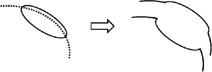
Figure 11: Illustration of the resonant torus and the additional curve is shown at left. The resonant torus can be reconstructed by the two pseudo-tori. One of the pseudo-tori (pseudo-torus 1) consists of the additional curve (except for the additional curve inside the resonant tours) and the upper part of the resonant torus as shown at upper right. Another one (pseudo-torus 2) consists of the additional curve (except the additional curve inside the resonant tours) and the lower part of the resonant torus as shown at lower right.

Figure 12: The same surface of section as shown in Fig.10. The solid lines represent the target tori derived by the numerical calculation of the orbits of test particles. The plus symbols show the reconstructed target tori containing resonant tori reconstructed using the procedure mentioned in the text. See the text for details.

Furthermore we confirmed that the torus-fitting method can reconstruct ”small islands” representing 7:6 resonant tori that appear around the 1:2 resonant torus. We can see from Figure 13 that the higher resonant orbit appears around the 1:2 resonant torus, and the torus-fitting method can be applied to these ”small islands” by the same procedures shown above. Fig.14 represents one of the ”small islands” in Fig.13, and plus symbols show the represent reconstructed small island using the torus-fitting method. Therefore, we conclude that the torus-fitting method is still useful to reconstruct minute structures.

Figure 13: The same surface of section as shown in Fig.9. The solid curves represent the target tori derived by the numerical calculations of the orbits of test particles. The “small islands” representing small resonant tori appear around 1:2 resonant torus.

Figure 14: The same surface of section as shown in Fig.13, but magnified around one of ”small islands”. The solid curves represent the target tori derived by the numerical calculation of the orbits of test particles. The plus symbols show the reconstructed target tori by using the torus-fitting method.

4.2 Some comments on the torus-fitting method

Before leaving this section, two subtle points concerning the torus-fitting method is considered. We first mention the application of the torus-fitting method to more complicated structures. Phase-space structures are in general complicated fractal structures under a general gravitational potential (Binney & Tremaine 1987). As shown in Fig.14, the torus-fitting algorithm is, in principal, applicable to such complicated phase-space structures, and this is one of the advantage of this method, while we need more CPU time for numerical calculations to get very fine structures in our method. However, we need not reproduce very fine structures on the phase-space in applying the fitting method to construct Galactic models that should be compared with observational data. This is, because, very fine structures cannot be reconstructed by the smearing effect due to observational errors. Hence, in the practical use of the fitting method, it is sufficient to construct torus structures whose scales on the phase-space are larger than those of the fine structures smeared by observational errors. So, in practical applications of constructing the torus structures of a Galactic model, it is enough to consider major orbits (box and loop orbits) and lower resonant orbits whose sizes of the tori are enough large to be considered.

We next mention angular variables. Although obtaining relations between angular variables and Cartesian coordinates is necessary to understand dynamical features of torus, this is irrelevant to the main subject. This is because that the purpose of this paper does not reproduce all characters of an invariant torus, but for obtaining relations between ${\bf J}$ and $({\bf x},{\bf p})$ through generating functions. In particular, the fact that we can reproduce any tori if some typical generating functions that reproduce some representative tori is important, and on this account we do not treat the angular variables. However, since winding number is an important quantity that represents dynamical features of an invariant torus, this is worth a mention in passing. In general, the winding number is a quantity that characterizes torus structure. For example, if a winding number is rational, the corresponding torus becomes a point or a set of points on a two-dimensional Poincare section, and we do not take account of these structures, because weights of these become zero when we construct a distribution function. On the other hand, if the winding number is irrational, the corresponding torus becomes a one-dimensional curve on a two-dimensional Poincare section. Because it is necessary to treat this case, the winding number is important when we use the torus-fitting method. As the purpose of this paper is to obtain the relation between ${\bf J}$ and $({\bf x},{\bf p})$, it is not necessary to show up the winding number of any torus, and we may leave the details to this topic.

5 Summary and Discussion

In this paper, we propose a new method, that is, the torus-fitting method for obtaining generating functions in two-dimensional Galactic potentials. We confirmed that the torus-fitting method works very well for constructing tori of major families of orbits in the two-dimensional logarithmic potential and Miyamoto-Nagai potential. In this method, the coefficients of generating functions are smooth functions of action variables ${\bf J^{\prime}}$ if the type of torus is the same type. Hence we can obtain coefficients of generating functions at any value of ${\bf J^{\prime}}$ by interpolating coefficients calculated at some typical values of ${\bf J^{\prime}}$. This fact reduces the computational time and the amount of memory required for computers. So this method is more practical compared with the direct numerical calculations of $J_{i}=\frac{1}{2\pi}\oint_{\gamma_{i}}{p}d{q}$ for obtaining the relations between the action variables of the target Hamiltonians and the Cartesian coordinates. Furthermore, the torus-fitting method is still applicable to resonant orbit families besides major orbit families, although we use the additional technique in which we use the pseudo-tori for constructing the target resonant tori. Hence the torus-fitting method is useful for analyzing a real Galactic system in which a lot of resonant orbits exist.

Here, we discuss applications of the torus-fitting method to observational data. To understand the dynamical structures of the Galaxy, we first assume a theoretical dynamical model, that is, a gravitational potential of the Galaxy, which should be compared with observations. If it is necessary for us to get the types of the orbits of each observed star and its value of ${\bf J^{\prime}}$ in the assumed model, how can we get them without direct numerical integrations of the orbits while the observations can provide only the positions and velocities of the stars at a given time? The strategy is given as follows: First, we suppose that the type of orbit of all observed stars is the box type as a trial. The use of the torus-fitting method makes it possible to convert the Cartesian coordinates, $({\bf x},{\bf p})$, of the observed stars into the action variables, ${\bf J^{\prime}}$. In this way, we can get the values of ${\bf J^{\prime}}$ of the observed stars if all orbits were box-type orbits. On the other hand, we have already estimated the allowed region of the values of ${\bf J^{\prime}}$ for the box-type orbit in the process of the construction of the generating functions when we apply the torus-fitting method to this assumed model. So if the estimated value of ${\bf J^{\prime}}$ of an observed star is included in this allowed region for the box type, we can recognize that the type of star is the box type and this value of ${\bf J^{\prime}}$ is the true value of the action variable of the star. Otherwise, the assumption that this star fs orbit is the box type is not true. So we again compute the value of ${\bf J^{\prime}}$ under the other supposition that the star’s orbit is a loop-type orbit or a resonant orbit by trial and error. In this way, we can finally derive the true value of ${\bf J^{\prime}}$ and the types of orbits.

If we assume that the Galaxy has a steady state, and almost all orbits of the celestial objects (the stars and dark matter) in the Galaxy are regular, then, as described in $\S 1$, the phase-space distribution function of the objects in the Galaxy is a function of three independent isolating integrals, which correspond to action variables. So we theoretically construct phase-space distribution functions of the action variables for any Galactic model depicts all orbits as regular. This means we need to recognize the values of the action variables of the observed stars when we compare a theoretically constructed phase-space distribution function with the distribution of the observed stars. Hence it is necessary and important to convert the Cartesian coordinate, $({\bf x},{\bf p})$, of the observed stars into the action variables, ${\bf J^{\prime}}$. As mentioned above, we can do so by the torus-fitting method.

It is apparent that the torus-fitting method cannot be applied to systems in which chaotic orbits are dominant in the phase space. However, if almost all orbits move for long periods around their nearby tori although the orbits are strictly chaotic, the orbits can be regarded as being approximately regular ones.This may be the case for some galactic bulges and some kinds of elliptical galaxies. The reason is that some galactic bulges and some elliptical galaxies have anisotropic velocity dispersions that cause the triaxial shape of the structures. This suggests that these systems have approximately three isolating integrals. That is, almost all orbits can be regarded as being approximately regular ones. If this guess is true, the torus-fitting method can be applied to these systems.

We finally discuss future work on the torus-fitting method. As a first step, we examined the two-dimensional potentials in this paper, although, a real galaxy generally has a three-dimensional potential. So we will try to apply the torus-fitting method to some three-dimensional potentials and a forthcoming paper will present this application. Modern space astrometry projects will provide us reliable information about stellar phase-space coordinates in the Galaxy, and so the torus-fitting method is useful for examining steady-state dynamical models of the Galaxy.

References

- Arnold (1989) Arnold V.I., 1989, Mathematical Methods of Classical Mechanics, Springer, Berlin
- Binney (1987) Binney J.J., Tremaine S., 1987, Galactic Dynamics, Princeton. Princeton University Press
- Binney et al. (1994) Binney J.J., Kumar S., 1993, MNRAS, 261, 584
- Binney (2002) Binney J.J., 2002, EAS Publications Series, Volume 2, Proceedings of “GAIA: A European Space Project”, ed. O. Bienayme & C. Turon, (Les Houches, France), 245
- Goldstein (2002) Goldstein, H., Poole C., Safko J., 2002, Classical Mechanics, 3nd ed. Peading, Penn. Addison-Wesley
- Kaasalainen (1994) Kaasalainen M., 1994, MNRAS, 268, 1041
- Kaasalainen (1995) Kaasalainen M., 1995, MNRAS, 275, 162
- Kaasalainen et al. (1994) Kaasalainen M., Binney J.J., 1994, MNRAS, 268, 1033
- McGill et al. (1990) McGill C., Binney J.J., 1990, MNRAS, 244, 634
- Miyamoto (1975) Miyamoto M., Nagai R., 1975, PASJ, 27, 533
- Sanders J. L. et al (2014) Sanders J. L., Binney J., 2014 preprint (arXiv:1401.3600)