On radiative corrections to polarization observables
in electron-proton scattering

Abstract

We consider radiative corrections to polarization observables in elastic electron-proton scattering, in particular, for the polarization transfer measurements of the proton form factor ratio $\mu G_{E}/G_{M}$. The corrections are of two types: two-photon exchange (TPE) and bremsstrahlung (BS); in the present work we pay special attention to the latter. Assuming small missing energy or missing mass cut-off, the correction can be represented in a model-independent form, with both electron and proton radiation taken into account. Numerical calculations show that the contribution of the proton radiation is not negligible. Overall, at high $Q^{2}$ and energies the total correction to $\mu G_{E}/G_{M}$ grows, but is dominated by TPE. At low energies both TPE and BS may be significant; the latter amounts to $\sim 0.01$ for some reasonable cut-off choices.

1 Introduction

Polarized and unpolarized elastic electron scattering are important sources of information about nucleon structure, which in this case reveals itself via electromagnetic form factors (FFs). Study of $Q^{2}$ dependence of the FFs allows, for example, to determine nucleon size and quark content, test phenomenological nucleon models, QCD predictions, and much more. However, the elastic scattering amplitude and the FFs are simply related only in the first order in $\alpha$, the electromagnetic interaction constant. An analysis of experimental data necessarily involves the calculation of higher-order effects, often called radiative corrections. In connection with the modern development of polarization transfer experiments [1] it became clear that higher-order corrections can seriously influence the FF measurements (see, e.g., Refs. [2, 3, 4]). Nevertheless, current cituation with the estimates of the radiative corrections to polarized $ep$ scattering is not quite satisfactory.

There are two distinct types of radiative corrections: 1) The corrections of the second order in $\alpha$ to the elastic amplitude. An example of such correction is two-photon exchange (TPE), and 2) The radiation of undetected (soft) photons, known as bremsstrahlung (BS) or radiative corrections in a narrow sense. It is well-known that both corrections are, in general, infra-red (IR) divergent and a finite cross-section value is obtained only after their summation. Hence both corrections should be considered in common. However, this was never done in calculations of the radiative corrections to polarization observables in $ep\to ep$. Thus, in Refs. [4] the correction was attributed entirely to TPE. On contrary, in Refs. [5, 6] the BS corrections were thoroughly analyzed, but the contribution of the box diagram (TPE) was ignored ”because its treatment … requires different methods”.

This became possible, since the IR-divergent term is factorizable; that is, it can be reduced to an overall spin-independent factor in the cross-section. Thus polarization observables, which are, in fact, ratios of some polarized cross-section to the unpolarized one, never suffer from the IR divergence; both TPE and BS corrections to such observables appear finite and may be calculated separately. Nevertheless, an arbitrary omission of one of them is obviously incorrect.

During last decade, TPE was studied rather thoroughly, and the corresponding amplitude was calculated by different authors in various approximations and kinematical conditions; we will not discuss it in detail here, but will just refer to the known results [4, 7, 8].

As to the BS, the most recent works on this subject [5, 6] still have some drawbacks. The main idea of the papers [5, 6] was an exact model-independent calculation of the BS effects. To achieve this, authors were to consider only the radiation by the electron, but not by the proton, since the latter depends on the details of the proton structure.

The neglection of the proton radiation seems well-justified at low momentum transfer, when the proton remains practically at rest. However, at typical experimental conditions in JLab [1] the final proton is relativistic, thus the electron and the proton are on an equal footing and their contributions to the BS should be of the same order of magnitude.

Even the full cancellation of the IR divergence is impossible without taking into account proton radiation. Namely, if the BS amplitude is ${\cal M}={\cal M}_{e}+{\cal M}_{p}$, where the subscript indicates radiating particle, then the IR divergence in $\int|{\cal M}_{e}|^{2}d\Gamma$ cancels with that of the electron vertex correction, the IR divergence in $\int|{\cal M}_{p}|^{2}d\Gamma$ — with the proton vertex correction, and the IR divergence in $\mathop{\rm Re}\nolimits\int{\cal M}_{e}{\cal M}_{p}^{*}d\Gamma$ — with the IR divergence of the TPE amplitude.

In the present paper we analyze radiative corrections to the polarization observables in $ep\to ep$. We take into account both TPE and BS, and for the latter include the radiation by the electron as well as by the proton. Certainly exact analytical and model-independent calculation of the proton radiation is impossible (still this is not needed for practical applications). However, we are able to obtain the result of such sort after the expansion in powers of photon energy, in the first non-vanishing order. The case of polarization transfer measurements of the proton FFs is considered in detail. Our approach is also applicable to other polarization experiments, e.g., measurements of beam-target asymmetry.

So as not to go into details of different experiments, we consider a simple idealized experiment in which the final proton is detected in a fixed direction, that is, the angular acceptance of the proton detector is very small. Both electron and proton energies are measured to determine missing energy $\Delta E$, and the event is counted as the elastic one if $\Delta E<r_{m}$, where $r_{m}$ is some cut-off. This is the way the elastic events were selected in the real experiments [1]. Authors of Refs. [5, 6] use a cut on the missing mass, which was not applied in Ref. [1]. This case is also considered in our paper and compared with the ”missing energy” approach.

To reduce inelastic background, one must choose reasonably small $r_{m}$. For example, to exclude pion production, $r_{m}$ should be restricted by $r_{m}<m_{\pi}\approx 140{\rm\ MeV}$. Therefore we have a small parameter $r_{m}$ or, more precisely, $r_{m}/M$ (where $M$ is the proton mass). We calculate the radiative correction in the first non-vanishing order in $r_{m}$. To this order, the low-energy theorem [9] allows us to obtain a model-independent result in the sense that it is expressed solely through on-shell proton FFs and their derivatives.

2 Bremsstrahlung cross-section

The process under consideration is

$$e(k)+p(p)\to e(k^{\prime})+p(p^{\prime})+\gamma(r).$$ (1)

We will also use the alternative notation $k_{a}$ for particle momenta, $k_{1}=k$, $k_{2}=p$, $k_{3}=k^{\prime}$, $k_{4}=p^{\prime}$. Throughout the paper space components of 4-vectors are denoted by boldface, e.g., ${\bf k}$, ${\bf p}$, etc. The electron and proton masses are $m$ and $M$, respectively. The cross-section is given by

$$d\sigma_{\gamma}=\frac{1}{(2\pi)^{5}}\delta(p\!+\!k\!-\!p^{\prime}\!-\!k^{\prime}\!-\!r)\frac{|{\cal M}|^{2}}{4M\epsilon}\frac{d{\bf p}^{\prime}}{2E^{\prime}}\frac{d{\bf k}^{\prime}}{2\epsilon^{\prime}}\frac{d{\bf r}}{2|{\bf r}|},$$ (2)

where ${\cal M}$ is the scattering amplitude, $\epsilon$ is initial electron energy in the lab. frame, $\epsilon^{\prime}$, $E^{\prime}$ and $|{\bf r}|$ are final electron, proton and photon energies. The appropriate summation/averaging over polarizations is implied. There are 9 variables here (${\bf p}^{\prime}$, ${\bf k}^{\prime}$ and ${\bf r}$), but due to the $\delta$-function only 5 are independent. We choose the independent integration variables to be ${\bf r}$ and ${\bf n}={\bf p}^{\prime}/|{\bf p}^{\prime}|$. This is convenient since ${\bf r}$ is small due to the missing energy cut $|{\bf r}|<r_{m}$ and ${\bf n}$ is fixed in our kinematics (see Introduction). All other kinematical quantities will be functions of ${\bf r}$ and ${\bf n}$, thus

$$k^{\prime}=k^{\prime}({\bf n},{\bf r}),\qquad p^{\prime}=p^{\prime}({\bf n},{\bf r}).$$ (3)

Putting ${\bf r}=0$, we return to purely elastic scattering, for which we denote

$$k^{\prime}_{0}=k^{\prime}({\bf n},0),\qquad p^{\prime}_{0}=p^{\prime}({\bf n},0).$$ (4)

Below we will make an expansion in powers of $r$. Requiring $k^{\prime 2}=m^{2}$ and $p^{\prime 2}=M^{2}$ it is easy to find

$$p^{\prime} = p^{\prime}_{0}+\delta p^{\prime}+O({\bf r}^{2}),$$ (5)

$$k^{\prime} = k^{\prime}_{0}-\delta p^{\prime}-r+O({\bf r}^{2}),$$ (6)

where

$$\delta p^{\prime}=2(k^{\prime}_{0}r)\frac{M^{2}p-(pp^{\prime}_{0})p^{\prime}_{0}}{MQ^{2}(\epsilon+M)}.$$ (7)

The $\delta$-function can be rewritten as

$$\delta(p\!+\!k\!-\!p^{\prime}\!-\!k^{\prime}\!-\!r)=J({\bf n},{\bf r})\cdot 2E^{\prime}\delta({\bf p}^{\prime}-{\bf p}^{\prime}({\bf n},{\bf r}))\cdot 2\epsilon^{\prime}\delta({\bf k}^{\prime}-{\bf k}^{\prime}({\bf n},{\bf r}))\cdot d\Omega_{{\bf n}},$$ (8)

where

$$J=\frac{1}{4M^{2}}\,\frac{[(pp^{\prime})^{2}-M^{4}]^{3/2}}{(pp^{\prime})(p^{\prime}k^{\prime})-M^{2}(pk^{\prime})}.$$ (9)

Thus we have

$$\frac{d\sigma_{\gamma}}{d\Omega_{{\bf n}}}=\frac{1}{(2\pi)^{2}}\frac{1}{4M\epsilon}\int|{\cal M}|^{2}\frac{Jd{\bf r}}{(2\pi)^{3}2|{\bf r}|}.$$ (10)

The amplitude ${\cal M}$ depends, in particular, on $p^{\prime}$ and $k^{\prime}$, which should be understood as functions of ${\bf r}$ and ${\bf n}$, Eqs. (5,6). Now we want to expand the integrand into the series in $r$, keeping two leading terms. The first term will be $O(1/|{\bf r}|)$ and corresponds to the so-called Mo&Tsai approximation [10]. Thus

$${\cal M}=\sqrt{4\pi\alpha}\,\varepsilon_{\mu}^{*}\left\{{\cal M}_{1}\left(\frac{k_{\mu}}{kr}-\frac{k^{\prime}_{\mu}}{k^{\prime}r}+\frac{Zp^{\prime}_{\mu}}{p^{\prime}r}-\frac{Zp_{\mu}}{pr}\right)+\delta{\cal M}_{\mu\nu}r_{\nu}+O(|{\bf r}|)\right\}=$$ (11)

$$=\sqrt{4\pi\alpha}\left\{{\cal M}_{1}\sum_{a}z_{a}\frac{k_{a}\varepsilon^{*}}{k_{a}r}+\sum_{a}\delta{\cal M}_{\mu\nu a}\frac{r_{\nu}\varepsilon_{\mu}^{*}}{k_{a}r}+O(|{\bf r}|)\right\},$$

where ${\cal M}_{1}$ is the elastic scattering amplitude in the Born approximation, $Z=1$ and is introduced, as usually, to distinguish electron and proton radiation (for positron-proton scattering we would put $Z=-1$), $z_{1}=1$, $z_{2}=-Z$, $z_{3}=-1$, $z_{4}=Z$, $\varepsilon_{\mu}$ is photon polarization vector, and $\delta{\cal M}_{\mu\nu a}$ is independent of $r$. Due to the low-energy theorem [9], $\delta{\cal M}_{\mu\nu a}$ can be expressed via ${\cal M}_{1}$, that is, via on-shell proton FFs (for more detail see the next section). The cross-section will be

$$d\sigma_{\gamma}\sim\int|{\cal M}|^{2}\frac{Jd{\bf r}}{(2\pi)^{3}2|{\bf r}|}=-4\pi\alpha|{\cal M}_{1}|^{2}\sum_{a,b}z_{a}z_{b}(k_{a}k_{b})\int\frac{J({\bf n},{\bf r})}{(k_{a}r)(k_{b}r)}\,\frac{d{\bf r}}{(2\pi)^{3}2|{\bf r}|}-$$ (12)

$$-4\pi\alpha J({\bf n},0)\cdot 2\mathop{\rm Re}\nolimits{\cal M}_{1}^{*}\sum_{a,b}\delta{\cal M}_{\mu\nu b}z_{a}k_{a\mu}\int\frac{r_{\nu}}{(k_{a}r)(k_{b}r)}\,\frac{d{\bf r}}{(2\pi)^{3}2|{\bf r}|}+O(r_{m}^{2}).$$

Note that the overall minus sign appears because the photon polarization sum is $\overline{\varepsilon_{\mu}\varepsilon^{*}_{\nu}}=-g_{\mu\nu}$. The first term is IR-divergent. It is well-known that the divergence cancels with the IR divergence in the TPE correction. Since that term has the same spin structure as the Born cross-section, it influences only the unpolarized cross-section (which is not of our interest), but not polarization observables. By the same reason, we do not need to expand $J({\bf n},{\bf r})$ under the first integral in the l.h.s. of Eq.(12).

So we should consider the second term. It is IR-finite, and the integrals it contains have the form

$$\phi_{ab\mu}=\int\frac{r_{\mu}}{(k_{a}r)(k_{b}r)}\,\frac{d{\bf r}}{(2\pi)^{3}2|{\bf r}|}=\frac{r_{m}}{16\pi^{3}}\int\frac{\rho_{\mu}}{(k_{a}\rho)(k_{b}\rho)}\,d\Omega_{{\bf\rho}},$$ (13)

where $\rho_{\mu}=r_{\mu}/|{\bf r}|$ depends on angular variables only. The integrals involving electron momenta are divergent at $m\to 0$:

$$\phi_{11},\phi_{33}\sim A+B\ln m^{2}+C/m^{2},\qquad\phi_{12},\phi_{13},\phi_{14},\phi_{32},\phi_{34}\sim A+B\ln m^{2}$$ (14)

(of course the $C/m^{2}$ terms cancel when computing any observable, but the logarithmic terms persist). These integrals are written out in Appendix A.

It is interesting to note that the second term in (12) can be viewed as a contribution coming from TPE with the amplitude

$$\delta{\cal M}=-4\pi\alpha\sum_{a,b}\delta{\cal M}_{\mu\nu b}z_{a}k_{a\mu}\phi_{ab\nu}.$$ (15)

Similarly to the TPE amplitude, the quantity $\delta{\cal M}$ can be expressed via scalar invariant amplitudes (generalized FFs). However, now we have to include not 6, but 8 FFs:

$${\cal M}={\cal M}_{1}+\delta{\cal M} = -\frac{4\pi\alpha Z}{q^{2}}\,\bar{u}^{\prime}\gamma_{\mu}u\,\bar{U}^{\prime}\gamma_{\nu}U\left\{(F_{1}+F_{2})g_{\mu\nu}-F_{2}\frac{P_{\mu}P_{\nu}}{M^{2}}+F_{3}\frac{P_{\mu}K_{\nu}}{M^{2}}+F_{4}\frac{K_{\mu}P_{\nu}}{m^{2}}-F_{5}\frac{K_{\mu}K_{\nu}}{m^{2}}\right\}-$$ (16)

$$-\frac{4\pi\alpha Z}{q^{2}}\left\{F_{6}\,\bar{u}^{\prime}\gamma_{5}u\,\bar{U}^{\prime}\gamma_{5}U+\frac{iF_{7}}{mq^{2}}\bar{u}^{\prime}\gamma_{5}u\,\bar{U}^{\prime}\hat{e}U+\frac{iF_{8}}{Mq^{2}}\bar{u}^{\prime}\hat{e}u\,\bar{U}^{\prime}\gamma_{5}U\right\},$$

where $u$, $u^{\prime}$ and $U$, $U^{\prime}$ are electron and proton spinors, respectively, $P=p+p^{\prime}$, $K=k+k^{\prime}$, $q=p^{\prime}-p$ and $\hat{e}=4\varepsilon^{\mu\nu\sigma\tau}\gamma_{\mu}P_{\nu}K_{\sigma}q_{\tau}$.

For the genuine TPE the amplitudes $F_{4,5,6}$ vanish in the zero electron mass limit and $F_{7,8}\equiv 0$, since these amplitudes violate T-invariance. On contrary, for the effective TPE describing BS, even if $m\to 0$, non-zero contributions arise in $F_{1-5}$ and $F_{7,8}$ (the amplitude $F_{6}$ is identically zero in our approximation).

The appearance of the T-violating amplitudes can be easily understood. In general, T-invariance connects the amplitudes for direct and time-reversed processes. For the elastic process the initial and final particles coincide, thus direct and reverse processes are, actually, the same process, and T-invariance imposes some constraints on its amplitude. For the BS an additional emitted photon breaks the symmetry between initial and final states, so the effective TPE amplitude need not necessarily be symmetric under time reversal.

Once we have converted BS into effective TPE, we may calculate both TPE and BS corrections to any observable through the same formulae (technically, this may be not the easiest way, but we find it interesting and feasible with symbolic calculation software).

The explicit expressions for the effective TPE amplitudes $F_{i}$ are given in Appendix B.

The detailed formulae for the cross-section and other observables in terms of the amplitudes $F_{i}$ are given in Appendix C. Here we write down only the correction to $G_{E}/G_{M}$ ratio, measured via polarization transfer. In the Born approximation, we have

$$R\equiv-\frac{S_{\perp}}{S_{\parallel}}\,\frac{\epsilon+\epsilon^{\prime}}{2M}\mathop{\rm tg}\nolimits\frac{\theta}{2}=\frac{G_{E}}{G_{M}},$$ (17)

where $\theta$ is lab. scattering angle and $S_{\perp}$ ($S_{\parallel}$) is the transverse (longitudinal) component of final proton polarization. The correction to this quantity is given by

$$\frac{F_{m}^{2}}{1-\frac{q^{2}}{4M^{2}}}\delta R=F_{2}\delta F_{m}-F_{m}\left(\delta F_{2}-\frac{4M^{2}}{\nu\!-\!q^{2}}\delta F_{4}\right)+\left(\frac{\nu F_{2}}{4M^{2}}-\frac{q^{2}}{\nu}F_{e}\right)\left(\delta F_{3}-\frac{4M^{2}}{\nu\!-\!q^{2}}\delta F_{5}+2\delta F_{8}\right)+$$ (18)

$$+\frac{8M^{2}}{\nu}F_{e}\delta F_{7}-\frac{2F_{1}F_{e}\delta F_{8}}{\nu q^{2}F_{m}}(\nu^{2}\!+\!q^{2}(4M^{2}\!-\!q^{2})),$$

where $\nu=4(p+p^{\prime})(k+k^{\prime})$ and the prefix $\delta$ indicates contribution of order $\alpha$. We have defined $F_{m}=F_{1}+F_{2}$ and $F_{e}=F_{1}+\frac{q^{2}}{4M^{2}}F_{2}$; these are not the same as the elastic FFs $G_{M}$ and $G_{E}$, since the former incorporate radiative corrections.

3 Bremsstrahlung amplitude in detail

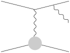
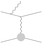
Figure 1: Bremsstrahlung diagrams.

The process amplitude is represented by the four diagrams (Fig. 1) and equals

$$\frac{{\cal M}}{(4\pi\alpha)^{3/2}Z} = \varepsilon^{*}\left(\frac{k^{\prime}}{k^{\prime}r}-\frac{k}{kr}-\frac{Zp^{\prime}}{p^{\prime}r}+\frac{Zp}{pr}\right)\bar{u}^{\prime}\gamma_{\mu}u\,\bar{U}^{\prime}\Gamma_{\mu}(q)U+$$

$$+ \left(\frac{1}{2k^{\prime}r}\bar{u}^{\prime}\hat{\varepsilon}^{*}\hat{r}\gamma_{\mu}u+\frac{1}{2kr}\bar{u}^{\prime}\gamma_{\mu}\hat{r}\hat{\varepsilon}^{*}u\right)\bar{U}^{\prime}\Gamma_{\mu}(q)U-$$

$$- Z\bar{u}^{\prime}\gamma_{\mu}u\,\bar{U}^{\prime}\left\{\frac{\kappa}{4M}\left([\hat{\varepsilon}^{*},\hat{r}]\frac{\hat{p}^{\prime}+M}{2p^{\prime}r}\Gamma_{\mu}(q)-\Gamma_{\mu}(q)\frac{\hat{p}+M}{2pr}[\hat{\varepsilon}^{*},\hat{r}]\right)+\right.$$

$$+ \left.\frac{1}{2p^{\prime}r}\hat{\varepsilon}^{*}\hat{r}\Gamma_{\mu}(q)+\frac{1}{2pr}\Gamma_{\mu}(q)\hat{r}\hat{\varepsilon}^{*}+\left(\frac{p^{\prime}\varepsilon^{*}}{p^{\prime}r}-\frac{p\varepsilon^{*}}{pr}\right)\left(\Gamma_{\mu}(q+r)-\Gamma_{\mu}(q)\right)\right\}U,$$

where

$$\Gamma_{\mu}(q)=\gamma_{\mu}\bar{F}_{1}(q^{2})-\frac{1}{4M}[\gamma_{\mu},\hat{q}]\bar{F}_{2}(q^{2}),\qquad\bar{F}_{i}(q^{2})=F_{i}(q^{2})/q^{2},\qquad\kappa=F_{2}(0).$$ (20)

The terms without $Z$ correspond to the electron, the terms containing $Z$ — to the proton radiation. In the latter case one needs to take into account off-shell effects. However to the needed order in $r$ they can be estimated in a model-independent way using gauge invariance (this is a sort of so-called low-energy theorem [9]). It turns out that these effects are absent in the leading order in $r$. The argumentation is quite similar to the one given in Refs [11, 9].

In short, let us assume that FFs in Eqs. (3,20) depend also on the proton virtuality $v$, $F_{i}(q^{2})\to F_{i}(q^{2},v)$. For the two last diagrams in Fig. 1, the virtualities are $2p^{\prime}r$ and $2pr$, respectively. Thus expanding in powers of $r$ we have

$$F_{i}(q^{2},v)=F_{i}(q^{2},0)+v\frac{\partial F_{i}}{\partial v}(q^{2},0)+O({\bf r}^{2}).$$ (21)

The first term is the on-shell FF and the second represents sought off-shell correction. After inserting (21) in the full expression for the ampltude (3), $v$ from the second term cancels with the proton propagator, thus the resulting contribution to the amplitude will be independent of $r$.

On the other hand, gauge invariance requires the amplitude to vanish upon the substitution $\varepsilon_{\mu}\to r_{\mu}$. This condition allows to determine the off-shell correction unambiguously. The straightforward calculation shows that the amplitude (3) is already gauge-invariant, thus ($r$-independent) off-shell correction should be identically zero.

Now we should carefully expand (3) in powers of $r$, following the pattern of Eq. (12). The first term in Eq. (3) seems to be proportional to the elastic Born amplitude, but this is not the case: the momenta of final particles $p^{\prime}$ and $k^{\prime}$ are not equal to the ”elastic” ones $p^{\prime}_{0}$ and $k^{\prime}_{0}$. To obtain the correct amplitude expansion, we use the formula

$$u(p+\delta p,S+\delta S)-u(p,S)\approx\frac{1}{2M}\left[\widehat{\delta p}-\gamma_{5}(M\widehat{\delta S}-p\delta S)\right]u(p,S),$$ (22)

where $p$ is particle momentum, $S$ is its spin 4-vector.

In all cases of our interest it is possible to use the above equation with $\delta S=0$. Indeed, if we consider an experiment with polarized target (beam-target asymmetry), then the polarization of final particles is not measured and $\delta S=0$. In the polarization-transfer experiment two quantities are measured: longitudinal and transverse polarizations of the final proton. Thus we should first insert $p^{\prime}$ in place of $p$ in Eq. (22). Since in our calculations the direction of final proton momentum is fixed and only its magnitude can vary, we easily have $\delta S=0$ for the measurement of transverse polarization and $\delta S=-\frac{S\delta p^{\prime}}{M^{2}}p^{\prime}$ for the longitudinal one. But the latter expression still yields zero contribution to the r.h.s. of (22). So we have

$$\bar{u}^{\prime}\gamma_{\mu}u\,\bar{U}^{\prime}\Gamma_{\mu}(q)U = \bar{u}^{\prime}_{0}\gamma_{\mu}u\,\bar{U}^{\prime}_{0}\Gamma_{\mu}(q_{0})U-$$ (23)

$$- \frac{1}{2m}\bar{u}^{\prime}_{0}(\widehat{\delta p^{\prime}}+\hat{r})\gamma_{\mu}u\,\bar{U}^{\prime}_{0}\Gamma_{\mu}(q_{0})U+$$

$$+ \frac{1}{2M}\bar{u}^{\prime}_{0}\gamma_{\mu}u\,\bar{U}^{\prime}_{0}\widehat{\delta p^{\prime}}\Gamma_{\mu}(q_{0})U+$$

$$+ \delta p^{\prime}_{\nu}\bar{u}^{\prime}_{0}\gamma_{\mu}u\,\bar{U}^{\prime}_{0}\frac{\partial\Gamma_{\mu}}{\partial q_{\nu}}(q_{0})U+O({\bf r}^{2}),$$

where $q_{0}=p_{0}^{\prime}-p$ and $\delta p^{\prime}$ is from Eq. (5). There is no need to expand the bracket $\frac{k^{\prime}}{k^{\prime}r}-\frac{k}{kr}-\frac{Zp^{\prime}}{p^{\prime}r}+\frac{Zp}{pr}$ in Eq. (3), since the resulting expression will be anyway proportional to the Born amplitude and does not influence polarization observables. The Born amplitude is (remember that the photon propagator is included into $\Gamma_{\mu}$)

$${\cal M}_{1}=-4\pi\alpha Z\,\bar{u}^{\prime}_{0}\gamma_{\mu}u\,\bar{U}^{\prime}_{0}\Gamma_{\mu}(q_{0})U.$$ (24)

The 2nd, 3rd, and 4th terms of Eq. (3) already contain the first power of $r$ in the numerators, thus here we may safely ignore the difference between $p^{\prime}$ and $p^{\prime}_{0}$, $U^{\prime}$ and $U^{\prime}_{0}$, etc.

Then we proceed to determining the effective TPE amplitudes $F_{i}$ and computing corrections to observables, as described in the previous section.

4 Results and discussion

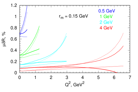
Figure 2: Bremsstrahlung correction to $\mu G_{E}/G_{M}$ ratio vs. $Q^{2}$ at different beam energies, as labelled on the plot. Solid — missing energy cut-off, dashed — mising mass cut-off; thick — full radiation, thin — electron only.

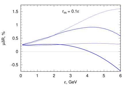
Figure 3: Bremsstrahlung correction to $\mu G_{E}/G_{M}$ ratio vs. beam energy at fixed scattering angle $90^{o}$. Curve types are the same as in Fig. 3.

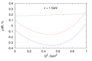
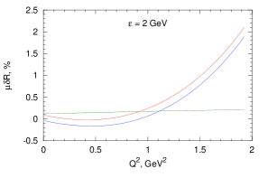
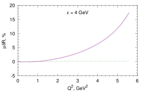
Figure 4: Radiative corrections to $\mu G_{E}/G_{M}$ ratio vs. $Q^{2}$, bremsstrahlung (green), TPE(blue), and total (red). Missing energy cut-off $r_{m}=0.1\epsilon$.

In all numerical calculations we use proton FF parameterization by Arrington et al. [12]. Everywhere below $\epsilon$ is initial electron energy (not to be confused with virtual photon polarization parameter).

Figure 3 displays the BS correction to $G_{E}/G_{M}$ ratio, as measured via polarization transfer [Eq. (17)], at four different beam energies. The missing energy cut-off is $r_{m}=0.15{\rm\ GeV}$. Since in our approximation the BS correction is proportional to $r_{m}$, the transition to another $r_{m}$ value is straightforward. The quantity shown in the figure is $\mu\,\delta R=\delta R(Q^{2})/R(Q^{2}=0)$. It is more convenient to plot than the relative correction $\delta R/R$, since $R$ approaches zero at $Q^{2}\sim 7{\rm\ GeV}^{2}$; therefore the relative correction strongly grows, even while $\delta R$ itself does not. The dashed curves are obtained in the ”missing mass” approach with the cut-off $(p^{\prime}+r)^{2}-M^{2}\leq 2Mr_{m}=u_{m}$. Thick curves results from the full calculation ($Z=1$), thin ones — including electron radiation only (dropping two last diagrams in Fig. 1 or putting $Z=0$ in the r.h.s. of Eq. (3)).

We see that the BS correction is typically quite small ($<1\%$), and has a tendency to drop as energy increases. This may indicate that the dimensionless expansion parameter is really not $r_{m}/M$, but rather $r_{m}/Q$ or $r_{m}/E$. The $Q^{2}$ dependence of the correction is weak, but at backward angles (when $Q^{2}$ is close to its maximum) the missing mass approach results in much larger correction. We also see that the significant part of the full correction is produced by proton radiation, especially at higher $\epsilon$ and $Q^{2}$.

The energy dependence of the BS correction at fixed lab. scattering angle $90^{\circ}$ is shown in Fig. 3. Here the missing energy cut-off is taken proportional to the incident electron energy: $r_{m}=0.1\epsilon$. The meaning of different curve types is the same as in Fig. 3. All four curves become close at $\epsilon\to 0$; this is clear, since at $\epsilon\to 0$ the final proton remains practically at rest ($p^{\prime}\approx p$) and thus does not radiate. At $\epsilon\gtrsim M$ full and ”electron only” calculations give very different results, as expected.

Comparing our results with the results of Refs. [5, 6], we note that the linearity of the BS correction in $r_{m}$ at small $r_{m}\ll M$ is clearly seen in the various figures from Refs. [5, 6] (note that $u_{m}=2Mr_{m}$), that is, the validity of the expansion in $r_{m}$ is supported by Refs. [5, 6] as well. At $\epsilon=4{\rm\ GeV}$ the correction obtained in the ”missing mass” approach, has the same behaviour and magnitude as shown in Fig. 4 of Ref. [5], but has opposite sign. The origin of this discrepancy is unclear.

In Fig. 4 we plot the total radiative correction, which is sum BS + TPE. The TPE correction was calculated according to Refs. [7, 8]. The BS is almost negligible with respect to TPE at $\epsilon\geq 2{\rm\ GeV}$; this is because the TPE correction grows with the energy, contrary to BS. At low energy the TPE correction is smaller and becomes comparable to BS. With the cut-off $r_{m}=0.1\epsilon$, used to produce Fig. 4, both corrections are negligible. However, the magnitude of the BS correction (contrary to the TPE one) substantially depends on the experimental details. If different cut-off is used in an experiment, the correction may become much larger (see e.g. Fig. 3). Thus we conclude that the BS corrections are of small importance for prospective high-$Q^{2}$ experiments, but may be significant and need to be more carefully analysed for low-$Q^{2}$ ones.

5 Conclusions

We have studied radiative corrections for the polarization transfer measurements of the proton FF ratio including both TPE and BS corrections. The latter was calculated assuming both electron and proton can radiate. Two approaches to the elastic event selection were considered: missing energy and missing mass cut-off.

Numerical calculation shows that:

1. The proton radiation yields a significant part of the BS corrrection at $\epsilon\gtrsim M$ in both ”missing energy” and ”missing mass” approaches.

2. In the ”missing mass” approach the correction strongly grows at large angles, whereas in the ”missing energy” approach it does not.

3. The BS correction is small at high energies ($\epsilon\gtrsim M$), where the TPE correction is much larger. However there is no final reliable estimate of the TPE amplitude in this region; this is an important open problem. The significance of the BS correction at low energies depends on experimental details; thus it should be checked separately for each case.

Appendix A Angular integrals $\phi_{ab\mu}$

The integral to calculate is

$$\phi_{ab\mu}=\frac{r_{m}}{16\pi^{3}}\int\frac{\rho_{\mu}d\Omega_{\rho}}{(k_{a}\rho)(k_{b}\rho)}=\frac{r_{m}}{16\pi^{3}}\bar{\phi}_{ab\mu},$$ (25)

where $\rho=(1,\boldsymbol{\rho})$ and ${\boldsymbol{\rho}}^{2}=1$. Obviously

$$\bar{\phi}_{ab\mu}=A_{ab}k_{a\mu}+A_{ba}k_{b\mu}+B_{ab}Me_{0\mu},$$ (26)

where $e_{0}=(1,{\bf 0})$. The coefficients $A$ and $B$ are easily expressed via the scalar integrals

$$\int\frac{d\Omega_{\rho}}{(k_{a}\rho)(k_{b}\rho)}=\frac{4\pi\varkappa_{a}\varkappa_{b}}{R}\ln\frac{k_{a}k_{b}+R}{m_{a}m_{b}},\qquad\int\frac{d\Omega_{\rho}}{k_{a}\rho}=\frac{4\pi}{\varkappa_{a}}\ln\frac{\epsilon_{a}+\varkappa_{a}}{m_{a}},$$ (27)

where $\varkappa_{a}=|{\bf k}_{a}|$, $m_{a}=\sqrt{k_{a}^{2}}$ and $R=\sqrt{(k_{a}k_{b})^{2}-m_{a}^{2}m_{b}^{2}}$. The final result is

$$\begin{split}&A_{ab}=\frac{4\pi}{\varkappa_{a}^{2}\varkappa_{b}\sin^{2}\theta}\left[(\epsilon_{a}\varkappa_{b}-\epsilon_{b}\varkappa_{a}\cos\theta)\frac{1}{R}\ln\frac{k_{a}k_{b}+R}{m_{a}m_{b}}-\ln\frac{\epsilon_{b}+\varkappa_{b}}{m_{b}}+\cos\theta\ln\frac{\epsilon_{a}+\varkappa_{a}}{m_{a}}\right],\\ &B_{ab}=\frac{4\pi}{M\varkappa_{a}^{2}\varkappa_{b}^{2}\sin^{2}\theta}\left[-R\ln\frac{k_{a}k_{b}+R}{m_{a}m_{b}}+(\epsilon_{a}\varkappa_{b}-\epsilon_{b}\varkappa_{a}\cos\theta)\ln\frac{\epsilon_{b}+\varkappa_{b}}{m_{b}}+(\epsilon_{b}\varkappa_{a}-\epsilon_{a}\varkappa_{b}\cos\theta)\ln\frac{\epsilon_{a}+\varkappa_{a}}{m_{a}}\right],\end{split}$$ (28)

where $\epsilon_{a}=k_{a0}$ and $\theta$ is the angle between ${\bf k}_{a}$ and ${\bf k}_{b}$.

There are three special cases. For $k_{a}=k_{b}$ we imply $\bar{\phi}_{aa\mu}=2A_{aa}k_{a\mu}+B_{aa}Me_{0\mu}$, with

$$A_{aa}=\frac{2\pi}{\varkappa_{a}^{3}}\left[\frac{\epsilon_{a}\varkappa_{a}}{m_{a}^{2}}-\ln\frac{\epsilon_{a}+\varkappa_{a}}{m_{a}}\right],\qquad B_{aa}=\frac{4\pi}{M\varkappa_{a}^{3}}\left[-\varkappa_{a}+\epsilon_{a}\ln\frac{\epsilon_{a}+\varkappa_{a}}{m_{a}}\right]$$ (29)

for $k_{b}=k_{2}\equiv p=Me_{0}$

$$A_{2a}\equiv 0,\qquad A_{a2}=-\frac{4\pi}{M\varkappa_{a}^{2}}\left[1-\frac{\epsilon_{a}}{\varkappa_{a}}\ln\frac{\epsilon_{a}+\varkappa_{a}}{m_{a}}\right],\qquad B_{a2}=\frac{4\pi}{M^{2}\varkappa_{a}^{2}}\left[\epsilon_{a}-\frac{m_{a}^{2}}{\varkappa_{a}}\ln\frac{\epsilon_{a}+\varkappa_{a}}{m_{a}}\right]$$ (30)

and for $k_{a}=k_{b}=k_{2}$

$$A_{22}\equiv 0,\qquad B_{22}=\frac{4\pi}{M^{3}}.$$ (31)

In Refs. [5, 6], authors consider a cut on the missing mass, instead of the missing energy, as an event selection criterion. This case is also covered by our approach. All ingredients of the calculation remain unchanged except the integrals $\phi_{ab\mu}$. The integrals can be rewritten in fully covariant form as

$$\phi_{ab\mu}=\frac{1}{(2\pi)^{3}}\int\limits_{pr\leq Mr_{m}}d^{4}r\,\delta(r^{2})\,\theta(r_{0})\,\frac{r_{\mu}}{(k_{a}r)(k_{b}r)}.$$ (32)

In the approach of Refs. [5, 6], the condition $pr\leq Mr_{m}$ is replaced by $(p+r^{\prime})^{2}-M^{2}=2p^{\prime}r\leq u_{m}$, thus the corresponding formulae can be obtained from the above by substitution $p\leftrightarrow p^{\prime}$, $r_{m}\to u_{m}/2M$.

Appendix B Effective TPE amplitudes

In this section we write down the effective TPE amplitudes $\delta F_{i}$, which correspond to the BS amplitude as discussed in Sec. 2. They are obtained as described in Sec. 3.

Below $t\equiv q^{2}$, $F_{m}^{\prime}=dF_{m}(q^{2})/dq^{2}$, $F_{2}^{\prime}=dF_{2}(q^{2})/dq^{2}$, $\kappa=F_{2}(0)$. The quantities $A_{ab}$ and $B_{ab}$ are defined in the previous Appendix. The electron mass $m$ is set to zero, except in front of $A_{11}$ and $A_{33}$, which diverge as $1/m^{2}$ (see Eqs.(13,14)). For brevity, we set $Z=1$ in the following equations. The $Z$ dependence can be easily restored by putting $A_{ab}\to z_{a}z_{b}A_{ab}$, $B_{ab}\to z_{a}z_{b}B_{ab}$, with $z_{1}=z_{3}=1$ and $z_{2}=z_{4}=Z$. Finally, $\delta F_{m}\equiv\delta F_{1}+\delta F_{2}$, and $\delta X$ is the auxilliary quantity which enter the formulae for $\delta F_{m}$ and $\delta F_{2}$.

$$\delta X=((4M^{2}-t)t-(8M^{2}-t)\nu)((t+\nu)A_{41}+(t-\nu)A_{43})-32\nu M^{4}A_{44}\\ +4t(4M^{2}-t)(4m^{2}A_{11}+2tA_{13}-(t+\nu)B_{13})\\ +t(12M^{2}-3t-\nu)((t+\nu)A_{14}+(t-\nu)A_{12})\\ +t(4M^{2}-t+\nu)((t+\nu)A_{32}+(t-\nu)A_{34})\\ -((4M^{2}-t)t+(8M^{2}-3t)\nu)((t+\nu)(B_{14}+B_{32})+(t-\nu)(B_{12}+B_{34}))\\ +8\nu{(2M^{2}-t)}^{2}B_{24}+8\nu M^{2}(2M^{2}-t)(2A_{42}-B_{22}-B_{44})$$ (33)

$$\frac{\pi\delta F_{m}}{\alpha tr_{m}}=\frac{1}{8}[8m^{2}F_{m}(A_{11}-A_{33})+4tF_{m}(A_{13}-A_{31}-B_{13})-(F_{2}-2F_{m})((t+\nu)(A_{14}-A_{32})+(t-\nu)(A_{12}-A_{34}))\\ -2(2M^{2}(F_{2}-2F_{m})+(t-\nu)F_{m})(A_{43}-B_{12}+B_{34})\\ -2(2M^{2}(F_{2}-2F_{m})+(t+\nu)F_{m})(A_{41}-B_{32}+B_{14})\\ +2tF_{2}(B_{14}+B_{34})-4M^{2}(F_{2}+F_{m})(2A_{44}-B_{22})\\ +2(4M^{2}F_{m}-t(F_{2}+2F_{m}))(A_{42}-B_{24})+(4M^{2}F_{1}+2tF_{2})B_{44}]+\frac{F_{m}^{\prime}}{4(4M^{2}-t+\nu)}\delta X$$ (34)

$$\frac{\pi\delta F_{2}}{\alpha tr_{m}}=\frac{1}{2}[F_{2}(2m^{2}(A_{11}-A_{33})+t(A_{13}-A_{31}-B_{13}))+M^{2}F_{m}(A_{43}+A_{41}-B_{12}-B_{32}+B_{14}+B_{34})]\\ +\frac{1}{4(4M^{2}-t)}[(tF_{2}-2M^{2}F_{m})((t+\nu)(A_{32}-A_{14}+B_{14})+(t-\nu)(A_{34}-A_{12}+B_{34}))\\ -((8M^{2}-t)F_{2}-2M^{2}F_{m})((t+\nu)(A_{41}-B_{32})+(t-\nu)(A_{43}-B_{12}))\\ +2(8M^{4}F_{2}+t^{2}F_{2}-2M^{2}t(5F_{2}-F_{m}))(A_{42}-B_{24})\\ +2M^{2}(tF_{2}-4M^{2}(3F_{2}-F_{m}))(2A_{44}-B_{22})+2M^{2}(4M^{2}F_{1}+t(3F_{2}-2F_{m}))B_{44}]\\ -\frac{\kappa}{4}\nu F_{1}[B_{14}-B_{34}]+\frac{4M^{2}F_{1}-tF_{2}+2(4M^{2}-t)tF_{2}^{\prime}}{8t(4M^{2}-t)(4M^{2}-t+\nu)}\delta X$$ (35)

$$\frac{\pi\delta F_{3}}{\alpha tr_{m}}=\frac{1}{4}[2M^{2}F_{2}(A_{43}+B_{32}-A_{41}-B_{12}+B_{14}-B_{34})-\kappa(tF_{2}+4M^{2}F_{1})(B_{14}-B_{34})]$$ (36)

$$\frac{\pi\delta F_{5}}{\alpha tr_{m}}=-\frac{\nu F_{m}}{2t(4M^{2}-t+\nu)}[4m^{2}tA_{11}+2t^{2}A_{13}+t(t+\nu)A_{14}+t(t-\nu)A_{12}\\ +2M^{2}((t+\nu)A_{41}+(t-\nu)A_{43})+8M^{4}A_{44}-2{(2M^{2}-t)}^{2}B_{24}\\ +(2M^{2}-t)(2tB_{13}+(t+\nu)(B_{14}+B_{32})+(t-\nu)(B_{12}+B_{34})-2M^{2}(2A_{42}-B_{22}-B_{44}))]$$ (37)

$$\frac{\pi\delta F_{8}}{\alpha tr_{m}}=\frac{1}{16}[(t+\nu)F_{2}(A_{14}+A_{32})+(t-\nu)F_{2}(A_{12}+A_{34})\\ -4M^{2}F_{1}(A_{41}-A_{43}-B_{12}+B_{32})-2(2M^{2}F_{1}+t(F_{2}+\kappa F_{m}))(B_{14}-B_{34})]$$ (38)

$$\delta F_{4}=\frac{({\nu}^{2}-t^{2})F_{2}-4M^{2}tF_{1}}{4M^{2}\nu F_{m}}\delta F_{5}$$ (39)

$$\delta F_{7}=\frac{t}{2\nu}\delta F_{5}$$ (40)

Appendix C Observables

In the case of double-polarization experiment the amplitude squared has the following general structure:

$$|\bar{\cal M}|^{2}=\alpha^{2}\left(a+b_{\mu}s_{\mu}+c_{\mu}S_{\mu}+d_{\mu\nu}s_{\mu}S_{\nu}\right),$$ (41)

where $s_{\mu}$ is incoming electron polarization and $S_{\mu}$ is the spin of the proton, either initial or final. The quantities $a$, $b$, $c$ and $d$ are quadratic functions of the generalized FFs $F_{i}$. The coefficients $b$ and $c$ have the form

$$b_{\mu}=\sum_{i,j}b_{ij\mu}\mathop{\rm Im}\nolimits F_{i}F_{j}^{*},\qquad c_{\mu}=\sum_{i,j}c_{ij\mu}\mathop{\rm Im}\nolimits F_{i}F_{j}^{*}.$$ (42)

and thus vanish in the Born approximation. They give rise to so-called single spin asymmetries; we do not need to consider them further. On contrary, the expressions for $a$ and $d$ involve the $\mathop{\rm Re}\nolimits$ sign

$$a=\sum_{i,j}a_{ij}\mathop{\rm Re}\nolimits F_{i}F_{j}^{*},\qquad d_{\mu\nu}=\sum_{i,j}d_{ij\mu\nu}\mathop{\rm Re}\nolimits F_{i}F_{j}^{*}$$ (43)

The corrections to double-polarization observables are related to $O(\alpha)$ terms in $d_{\mu\nu}$. The detailed expression for $d_{\mu\nu}$, corresponding to the square of ampltude (16), is written below. In the Born approximation there are only two non-zero FFs, $F_{1}$ and $F_{2}$. Thus all terms, proportional to $F_{i}F_{j}^{*}$ with $i,j\geq 3$ are dropped — they are small as $O(\alpha^{2})$. We have

$$d_{\mu\nu}=-\frac{2}{mM}\mathop{\rm Re}\nolimits\left\{4m^{2}M^{2}q^{2}g_{\mu\nu}^{\perp}F_{m}^{2}+4m^{2}q^{2}[P_{\mu}P_{\nu}-P^{2}g_{\mu\nu}^{\perp}]F_{m}F_{2}-m^{2}q^{2}[4K_{\mu}P_{\nu}-\nu g_{\mu\nu}^{\perp}]F_{m}F_{3}\right.$$

$$-M^{2}q^{2}[4P_{\mu}K_{\nu}-\nu g_{\mu\nu}^{\perp}]F_{m}F_{4}+4M^{2}q^{2}[K_{\mu}K_{\nu}-K^{2}g_{\mu\nu}^{\perp}]F_{m}F_{5}-e_{\mu}e_{\nu}F_{2}F_{5}/4$$

$$+8M^{2}F_{7}\left[4m^{2}F_{m}K_{\mu}P_{\nu}-(\nu K_{\mu}+q^{2}P_{\mu})\left(F_{e}K_{\nu}+\tfrac{\nu F_{2}}{4M^{2}}P_{\nu}\right)\right]$$

$$\left.+8m^{2}F_{8}\left[q^{2}F_{m}P_{\mu}K_{\nu}+(\nu F_{1}P_{\mu}-4M^{2}F_{e}K_{\mu})P_{\nu}\right]\right\},$$ (44)

where $g_{\mu\nu}^{\perp}=g_{\mu\nu}-q_{\mu}q_{\nu}/q^{2}$, $e_{\mu}=4\varepsilon^{\mu\nu\sigma\tau}P_{\nu}K_{\sigma}q_{\tau}$. Contracting $d_{\mu\nu}$ with $s_{\mu}=k_{\mu}/m-mp_{\mu}/pk$, which corresponds to the longitudinally polarized electron, we obtain the final proton polarization

$$S_{\mu}\sim AK_{\mu}+BP_{\mu},$$ (45)

with

$$A = 4M^{2}F_{m}^{2}-(4M^{2}\!-\!q^{2})F_{m}\left(F_{2}-\frac{4M^{2}}{\nu\!-\!q^{2}}F_{4}\right)+$$ (46)

$$+\nu F_{m}\left(F_{3}+2F_{8}-\frac{4M^{2}}{\nu\!-\!q^{2}}F_{5}\right)+8M^{2}F_{e}F_{7}\left(1+\frac{4M^{2}}{\nu\!-\!q^{2}}\right)$$

$$B = \nu F_{m}\left(F_{2}-\frac{4M^{2}}{\nu\!-\!q^{2}}F_{4}\right)+q^{2}F_{m}\left(F_{3}+2F_{8}-\frac{4M^{2}}{\nu\!-\!q^{2}}F_{5}\right)-$$ (47)

$$-\frac{2F_{7}}{\nu\!-\!q^{2}}[4M^{2}(\nu F_{e}-q^{2}F_{m})-\nu^{2}F_{2}]+2F_{1}F_{8}(4M^{2}\!-\!q^{2}\!+\!\nu^{2}/q^{2}).$$

From this it is easy to obtain Eq. (18).