Efficient Computation of the Well-Founded Semantics over Big Data

Abstract

Data originating from the Web, sensor readings and social media result in increasingly huge datasets. The so called Big Data comes with new scientific and technological challenges while creating new opportunities, hence the increasing interest in academia and industry. Traditionally, logic programming has focused on complex knowledge structures/programs, so the question arises whether and how it can work in the face of Big Data. In this paper, we examine how the well-founded semantics can process huge amounts of data through mass parallelization. More specifically, we propose and evaluate a parallel approach using the MapReduce framework. Our experimental results indicate that our approach is scalable and that well-founded semantics can be applied to billions of facts. To the best of our knowledge, this is the first work that addresses large scale nonmonotonic reasoning without the restriction of stratification for predicates of arbitrary arity.

1 Introduction

Huge amounts of data are being generated at an increasing pace by sensor networks, government authorities and social media. Such data is heterogeneous, and often needs to be combined with other information, including database and web data, in order to become more useful. This big data challenge is at the core of many contemporary scientific, technological and business developments.

The question arises whether the reasoning community, as found in the areas of knowledge representation, rule systems, logic programming and semantic web, can connect to the big data wave. On the one hand, there is a clear application scope, e.g. deriving higher-level knowledge, assisting decision support and data cleaning. But on the other hand, there are significant challenges arising from the area’s traditional focus on rich knowledge structures instead of large amounts of data, and its reliance on in-memory methods. The best approach for enabling reasoning with big data is parallelization, as established e.g. by the LarKC project (Fensel et al. (2008)).

As discussed in (Fensel et al. (2008)), reasoning on the large scale can be achieved through parallelization by distributing the computation among nodes. There are mainly two proposed approaches in the literature, namely rule partitioning and data partitioning (Soma and Prasanna (2008)).

In the case of rule partitioning, the computation of each rule is assigned to a node in the cluster. Thus, the workload for each rule (and node) depends on the structure and the size of the given rule set, which could possibly prevent balanced work distribution and high scalability. On the other hand, for the case of data partitioning, data is divided in chunks with each chunk assigned to a node, allowing more balanced distribution of the computation among nodes.

Parallel reasoning, based on data partitioning, has been studied extensively. In particular, MARVIN (Oren et al. (2009)), follows the divide-conquer-swap strategy in which triples are being swapped between nodes in the cluster in order to achieve balanced workload. MARVIN implements the SpeedDate method, presented in (Kotoulas et al. (2010)), where authors pointed out and addressed the scalability challenge posed by the highly uneven distribution of Semantic Web data.

WebPIE (Urbani et al. (2012)) implements forward reasoning under RDFS and OWL ter Horst semantics over the MapReduce framework (Dean and Ghemawat (2004)) scaling up to 100 billion triples. In (Goodman et al. (2011)) authors present RDFS inference scaling up to 512 processors with the ability to process, entirely in-memory, 20 billion triples.

FuzzyPD (Liu et al. (2011, 2012)) is a MapReduce based prototype system allowing fuzzy reasoning in OWL $pD^{*}$ with scalability of up to 128 process units and over 1 billion triples. Description logic in the form of $\mathcal{EL+}$ have been studied in (Mutharaju et al. (2010)). The authors parallelize an existing algorithm for $\mathcal{EL+}$ classification by converting it into MapReduce algorithms, while experimental evaluation was deferred to future work.

(Tachmazidis et al. (2012)) deals with defeasible logic for unary predicates scaling up to billions of facts, while authors extend their approach in (Tachmazidis et al. (2012)) for predicates of arbitrary arity, under the assumption of stratification, scaling up to millions of facts. Finally, the computation of stratified semantics of logic programming that can be applied to billions of facts is reported in (Tachmazidis and Antoniou (2013)).

In this paper, we propose a parallel approach for the well-founded semantics computation using the MapReduce framework. Specifically, we adapt and incorporate the computation of joins and anti-joins, initially described in (Tachmazidis and Antoniou (2013)). The crucial difference is that in this paper recursion through negation is allowed, meaning that the well-founded model can contain undefined atoms. A challenge in this respect is that materializing the Herbrand base is impractical in the context of big data. To overcome this scalability barrier we require programs to be safe and apply a reasoning procedure that allows closure calculation based on the consecutive computation of true and unknown literals, requiring significantly less information. Experimental results highlight the advantages of the applied optimizations, while showing that our approach can scale up to 1 billion facts even on a modest computational setup.

The rest of the paper is organized as follows. Section 2 introduces briefly the MapReduce framework, the well-founded semantics and the alternating fixpoint procedure. Join and anti-join operations for the well-founded semantics are described in Section 3. Section 4 provides a parallel implementation over the MapReduce framework, while experimental results are presented in Section 5. We conclude and discuss future directions in Section 6.

2 Preliminaries

2.1 MapReduce Framework

MapReduce is a framework for parallel processing over huge datasets (Dean and Ghemawat (2004)). Processing is carried out in a map and a reduce phase. For each phase, a set of user-defined map and reduce functions are run in parallel. The former performs a user-defined operation over an arbitrary part of the input and partitions the data, while the latter performs a user-defined operation on each partition.

MapReduce is designed to operate over key/value pairs. Specifically, each $Map$ function receives a key/value pair and emits a set of key/value pairs. Subsequently, all key/value pairs produced during the map phase are grouped by their key and passed to reduce phase. During the reduce phase, a $Reduce$ function is called for each unique key, processing the corresponding set of values.

Let us illustrate the wordcount example. In this example, we take as input a large number of documents and calculate the frequency of each word. The pseudo-code for the $Map$ and $Reduce$ functions is provided in A.

Consider the following documents as input:

Doc1: “Hello world.”

Doc2: “Hello MapReduce.”

During map phase, each map operation gets as input a line of a document. $Map$ function extracts words from each line and emits pairs of the form $<$w, “1”$>$ meaning that word w occurred once (“1”), namely the following pairs:

$<$Hello, 1$>$

$<$world, 1$>$

$<$Hello, 1$>$

$<$MapReduce, 1$>$

MapReduce framework will perform grouping/sorting resulting in the following intermediate pairs:

$<$Hello, $<$1,1$>$$>$	$<$world, 1$>$	$<$MapReduce, 1$>$

During the reduce phase, the $Reduce$ function sums up all occurrence values for each word emitting a pair containing the word and the frequency of the word. Thus, the reducer with key:

Hello will emit $<$Hello, 2$>$
world will emit $<$world, 1$>$
MapReduce will emit $<$MapReduce, 1$>$

2.2 Well-Founded Semantics

In this section we provide the definition of the well-founded semantics (WFS) as it was defined in (Gelder et al. (1991)).

Definition 2.1

(Gelder et al. (1991)) A general logic program is a finite set of general rules, which may have both positive and negative subgoals. A general rule is written with its head, or conclusion on the left, and its subgoal (body), if any to the right of the symbol “$\leftarrow$”, which may be read “if”. For example,

p(X) $\leftarrow$ a(X), not b(X).

is a rule in which p(X) is the head, a(X) is a positive subgoal, and b(X) is a negative subgoal. This rule may be read as “p(X) if a(X) and not b(X)”. A Horn rule is one with no negative subgoals, and a Horn logic program is one with only Horn rules.

We use the following conventions. A logical variable starts with a capital letter while a constant or a predicate starts with a lowercase letter. Note that functions are not allowed. A predicate of arbitrary arity will be referred as a literal. Constants, variables and literals are terms. A ground term is a term with no variables. The Herbrand universe is the set of constants in a given program. The Herbrand base is the set of ground terms that are produced by the substitution of variables with constants in the Herbrand universe. In this paper, we will refer to Horn rules also as definite rules, likewise Horn programs will also be referred to as definite programs.

Definition 2.2

(Gelder et al. (1991)) Given a program P, a partial interpretation I is a consistent set of literals whose atoms are in the Herbrand base of P. A total interpretation is a partial interpretation that contains every atom of the Hebrand base or its negation. We say a ground (variable-free) literal is true in I when it is in I and say it is false in I when its complement is in I. Similarly, we say a conjunction of ground literals is true in I if all of the literals are true in I, and is false in I if any of its literals is false in I.

Definition 2.3

(Gelder et al. (1991)) Let a program P, its associated Herbrand base H and a partial interpretation I be given. We say A $\subseteq$ H is an unfounded set (of P) with respect to I if each atom p $\in$ A satisfies the following condition: For each instantiated rule $R$ of P whose head is p, (at least) one of the following holds:

1. Some (positive or negative) subgoal of the body is false in I.

2. Some positive subgoal of the body occurs in A.

A literal that makes (1) or (2) above true is called a witness of unusability for rule $R$ (with respect to I).

Theorem 2.1

(Gelder et al. (1991)) The data complexity of the well-founded semantics for function-free programs is polynomial time.

In this paper, we require each rule to be safe, that is, each variable in a rule must occur (also) in a positive subgoal. Safe programs consist of safe rules only. This safety criterion is an adaptation of range restriction (Nicolas (1982)), which guarantees the important concept of domain independence, originally studied in deductive databases (see for example (Abiteboul et al. (1995))). Apart from this semantic property, the safety condition implicitly also enforces a certain locality of computation, which is important for our proposed method, as we shall discuss in Section 4.2.

2.3 Alternating Fixpoint Procedure

In this section, we provide the definition of the alternating fixpoint procedure as it was defined in (Brass et al. (2001)).

Definition 2.4

(Brass et al. (2001)) For a set S of literals we define the following sets:

pos(S)	:=	{A $\in$ S $|$ A is a positive literal },
neg(S)	:=	{A $|$ not A $\in$ S}.

Definition 2.5

(Brass et al. (2001)) (Extended Immediate Consequence Operator)
Let P be a normal logic program. Let I and J be sets of ground atoms. The set T_P,J(I) of immediate consequences of I w.r.t. P and J is defined as follows:

TP,J(I) := {A $|$ there is A $\leftarrow$ $\mathcal{B}$ $\in$ ground(P) with pos($\mathcal{B}$) $\subseteq$ I and neg($\mathcal{B}$) $\cap$ J = $\emptyset$}.

If P is definite, the set J is not needed and we obtain the standard immediate consequence operator T_P by T_P(I) $=$ T_P,∅(I).

For an operator $T$ we define $T$ $\uparrow$ $0$ $:=$ $\emptyset$ and $T$ $\uparrow$ $i$ $:=$ $T(T\uparrow i-1)$, for $i>0$. lfp($T$) denotes the least fixpoint of $T$, i.e. the smallest set $S$ such that $T(S)=S$.

Definition 2.6

(Brass et al. (2001)) (Alternating Fixpoint Procedure)
Let P be a normal logic program. Let P⁺ denote the subprogram consisting of the definite rules of P. Then the sequence (K_i,U_i)_i≥0 with set K_i of true (known) facts and U_i of possible (unknown) facts is defined by:

	K0 $:=$ lfp(T${}_{P^{+}}$)	U0 $:=$ lfp(T${}_{P,K_{0}}$)
$i>0:$	Ki $:=$ lfp(T${}_{P,U_{i-1}}$)	Ui $:=$ lfp(T${}_{P,K_{i}}$)

The computation terminates when the sequence becomes stationary, i.e., when a fixpoint is reached in the sense that (K_i,U_i) = (K_i+1,U_i+1). This computation schema is called the Alternating Fixpoint Procedure (AFP).

We rely on the definition of the well-founded partial model W${}^{*}_{p}$ of P as given in (Gelder et al. (1991)).

Theorem 2.2

(Brass et al. (2001)) (Correctness of AFP)
Let the sequence (K_i,U_i)_i≥0 be defined as above. Then there is a $j\geq 0$ such that (K_j,U_j)= (K_j+1,U_j+1). The well-founded model W${}^{*}_{p}$ of P can be directly derived from the fixpoint (K_j,U_j), i.e.,

W${}^{*}_{p}$ = {L $|$	L is a positive ground literal and L $\in$ Kj or
	L is a negative ground literal not A and A $\in$ BASE(P) $-$ Uj},

where BASE(P) is the Herbrand base of program P.

Lemma 2.1

(Brass et al. (2001)) (Monotonicity)
Let the sequence (K_i,U_i)_i≥0 be defined as above. Then the following holds for $i\geq 0:$
K_i $\subseteq$ K_i+1, U_i $\supseteq$ U_i+1, K_i $\subseteq$ U_i.

3 Computing T_P,J(I)

Consider the following program:

p(X,Y) $\leftarrow$ a(X,Z), b(Z,Y), not c(X,Z), not d(Z,Y).

Here p(X,Y) is our final goal, a(X,Z) and b(Z,Y) are positive subgoals, while c(X,Z) and d(Z,Y) are negative subgoals. In order to compute our final goal p(X,Y) we need to ensure that {a(X,Z), b(Z,Y)} $\subseteq$ I and {c(X,Z), d(Z,Y)} $\cap$ J = $\emptyset$ (see Definition 2.5), namely both a(X,Z) and b(Z,Y) are in I while none of c(X,Z) and d(Z,Y) is found in J.

As positive subgoals depend on I we can group them into a positive goal. A positive goal consists of a new predicate (say ab) that contains as arguments the union of two sets: (a) all the arguments of the final goal (X,Y) and (b) all the common arguments between positive and negative subgoals (X,Z,Y), namely we need to compute ab(X,Z,Y). The final goal (p(X,Y)) consists of all values of the positive goal (ab(X,Z,Y)) that do not match any of the negative subgoals (c(X,Z) and d(Z,Y)) on their common arguments (X,Z and Z,Y respectively).

3.1 Positive goal calculation

Consider the following program:

p(X,Y) $\leftarrow$ a(X,Z), b(Z,Y), not c(X,Z), not d(Z,Y).

where

I = {a(1,2), a(1,3), b(2,4), b(3,5)}

J = {c(1,2), d(2,3)}

A single join (Cluet and Moerkotte (1994)), calculating the positive goal ab(X,Z,Y), can be performed as described below. The pseudo-code for the $Map$ and $Reduce$ functions is provided in A. Note that we use only literals from I.

The $Map$ function will emit pairs of the form $<$Z,(a,X)$>$ for predicate a and $<$Z,(b,Y)$>$ for predicate b, namely the following pairs:

$<$2, (a,1)$>$

$<$3, (a,1)$>$

$<$2, (b,4)$>$

$<$3, (b,5)$>$

MapReduce framework will perform grouping/sorting resulting in the following intermediate pairs:

$<$2, $<$(a,1), (b,4)$>$$>$

$<$3, $<$(a,1), (b,5)$>$$>$

During the reduce phase we match predicates a and b on their common argument (which is the key) and use the values to emit positive goals. Thus, the reducer with key:

2 will emit ab(1,2,4)

3 will emit ab(1,3,5)

Note that we need to filter out possibly occurring duplicates as soon as possible because they will produce unnecessary duplicates as well, affecting the overall performance. The pseudo-code and a brief description of duplicate elimination are provided in A.

For rules with more than one join between positive subgoals we need to apply multi-joins (multi-way join).

Consider the following program:

q(X,Y) $\leftarrow$ a(X,Z), b(Z,W), c(W,Y), not d(X,W).

We can compute the positive goal (abc(X,W,Y)) by applying our approach for single join twice. First, we need to join a(X,Z) and b(Z,W) on Z, producing a temporary literal (say ab(X,W)), and then join ab(X,W) and c(W,Y) on W producing the positive goal (abc(X,W,Y)). Once abc(X,W,Y) is calculated, we proceed with calculating the final goal q(X,Y) by retaining all the values of abc(X,W,Y) that do not match d(X,W) on their common arguments (X,W).

For details on single and multi-way join, readers are referred to literature. More specifically, multi-way join has been described and optimized in (Afrati and Ullman (2010)). In order to achieve an efficient implementation, optimizations in (Afrati and Ullman (2010)) should be taken into consideration.

3.2 Final goal calculation

Consider the program mentioned at the beginning of Section 3.1. By calculating the positive goal ab(X,Z,Y) we obtain the following knowledge:

ab(1,2,4)

ab(1,3,5)

In order to calculate the final goal (p(X,Y)) we need to perform an anti-join (Cluet and Moerkotte (1994)) between ab(X,Z,Y) and each negative subgoal (c(X,Z) and d(Z,Y)). Note that to perform an anti-join we use only the previously calculated positive goal (ab(X,Z,Y)) and literals from J.

We start by performing an anti-join between ab(X,Z,Y) and c(X,Z) on their common arguments (X,Z), creating a new literal (say abc(X,Z,Y)), which contains all the results from ab(X,Z,Y) that are not found in c(X,Z), as described below. The pseudo-code for the $Map$ and $Reduce$ functions is provided in A.

The $Map$ function will emit pairs of the form $<$(X,Z),(ab,Y)$>$ for predicate ab and $<$(X,Z),c$>$ for predicate c (while predicate d will be taken into consideration during the next anti-join), namely the following pairs:

$<$(1,2), (ab,4)$>$

$<$(1,3), (ab,5)$>$

$<$(1,2), c$>$

MapReduce framework will perform grouping/sorting resulting in the following intermediate pairs:

$<$(1,2), $<$(ab,4), (c)$>$$>$

$<$(1,3), (ab,5)$>$

During the reduce phase we output values of the predicate ab only if it is not matched by predicate c on their common arguments (which are contained in the key) and emit abc(X,Z,Y). Thus, the reducer with key:

(1,2) will have no output

(1,3) will emit abc(1,3,5)

In order to calculate the final goal (p(X,Y)), we need to perform an additional anti-join between abc(X,Z,Y) and d(Z,Y) on their common arguments (Z,Y). Here, abc(1,3,5) and d(2,3) do not match on their common arguments (Z,Y) as (3,5) $\neq$ (2,3). Thus, our calculated final goal is p(1,5).

4 Computing the Well-Founded Semantics

In this section we describe an optimized implementation for the calculation of the well-founded semantics. A naive implementation is considered as one following Definition 2.6 while ignoring the monotonicity properties of the well-founded semantics (see Lemma 2.1).

4.1 Optimized implementation

A naive implementation would introduce unnecessary overhead to the overall computation since it comes with the overhead of reasoning over and storage of overlapping sets of knowledge. A more refined version of both WFS fixpoint and least fixpoint of T_P,J(I) is defined in Algorithm 1 and Algorithm 2 respectively.

1:opt_WFS_fixpoint(P): $\triangleright$ input: program P

2:K₀ = opt_lfp(P+, $\emptyset$, $\emptyset$); $\triangleright$ output: set of literals K_i-1, U_i-1

3:i = 0;

4:repeat

5:     U_i = K_i $\cup$ opt_lfp(P, K_i, K_i);

6:     i++; $\triangleright$ next “inference step”

7:     K_i = K_i-1 $\cup$ opt_lfp(P, K_i-1, U_i-1);

8:until K_i-1.size() == K_i.size()

9:return K_i-1, U_i-1;

Algorithm 1 Optimized WFS fixpoint

1:opt_lfp(P, I, J): $\triangleright$ precondition: I $\subseteq$ lfp(T_P,J($\emptyset$))

2:S = $\emptyset$; $\triangleright$ input: program P, set of literals I and J

3:new = $\emptyset$; $\triangleright$ output: set of literals S (lfp(T_P,J(I) - I)

4:repeat

5:     S = S $\cup$ new;

6:     new = T(P, (I $\cup$ S), J);

7:     new = new - (I $\cup$ S);

8:until new == $\emptyset$

9:return S;

Algorithm 2 Optimized least fixpoint of T_P,J(I)

Our first optimization is the changed calculation of the least fixpoint of T_P,J(I) (opt_lfp), which is depicted in Algorithm 2. Instead of calculating the least fixpoint starting from I $=$ $\emptyset$, for a given program P and a set of literals J, we allow the calculation to start from a given I, provided that I $\subseteq$ lfp(T_P,J($\emptyset$)), and return only the newly inferred literals (S) that led us to the least fixpoint. Thus, the actual set of literals that the least fixpoint of T_P,J(I) consists of is I $\cup$ S. In order to reassure correctness we need to take into consideration both I and S while calculating the least fixpoint, namely new literals are inferred by calculating T_P,J(I $\cup$ S). However, we use a temporary set of inferred literals (new) in order to eliminate duplicates (new $=$ new $-$ (I $\cup$ S)) prior to adding newly inferred literals to the set S (S $=$ S $\cup$ new). Note that the set of literals I remains unchanged when the optimized least fixpoint is calculated.

The optimized version of the least fixpoint is used, in Algorithm 1, for the computation of each set of literals K and U. K₀ is a special case where we start from I $=$ $\emptyset$ and J $=$ $\emptyset$, and thus, unable to fully utilize the advantages of the optimized least fixpoint.

The proposed optimizations are mainly based on the monotonicity of the well-founded semantics as given in Lemma 2.1. Note that in this section, the indices of the sets K and U found in Lemma 2.1 are adjusted to the indices used in Algorithm 1 in order to facilitate our discussion.

Since K_i $\subseteq$ U_i, for $i\geq 0$ (see Lemma 2.1), the computation of U_i can start from K_i, namely I $=$ K_i. Thus, instead of recomputing all literals of K_i while calculating U_i, we can use them to speed up the process. Note that the actual least fixpoint of U_i is the union of sets K_i and opt_lfp(P, K_i, K_i), as the optimized least fixpoint computes only new literals (which are not included in given I).

Since K_i-1 $\subseteq$ K_i, for $i\geq 1$ (see Lemma 2.1), the computation of K_i can start from K_i-1, namely I $=$ K_i-1. Once opt_lfp(P, K_i-1, U_i-1) is computed, we append it to our previously stored knowledge K_i-1, resulting in K_i. In addition, a WFS fixpoint is reached when K_i-1 $=$ K_i, namely when K_i-1 and K_i have the same number of literals.

Proof 4.1.

If K_i-1 $=$ K_i, for $i\geq 1$, then
U_i-1 $=$ K_i-1 $\cup$ opt_lfp(P, K_i-1, K_i-1) $=$ K_i $\cup$ opt_lfp(P, K_i, K_i) $=$ U_i
Thus, fixpoint is reached as (K_i-1,U_i-1) =(K_i,U_i).

According to Theorem 2.2, having reached WFS fixpoint at step $i$, we can determine which literals are true, undefined and false as follows: (a) true literals, denoted by K_i, (b) undefined literals, denoted by U_i $-$ K_i and (c) false literals, denoted by BASE(P) $-$ U_i.

Although for K_i calculation only new literals are inferred during each “inference step”, for U_i we have to recalculate a subset of literals that can be found in U_i-1, as literals in U_i-1 $-$ K_i-1 are discarded prior to the computation of U_i. However, the computational overhead coming from the calculation of opt_lfp(P, K_i, K_i) reduces over time since the set of literals in U_i $-$ K_i becomes smaller after each “inference step” due to K_i-1 $\subseteq$ K_i and U_i-1 $\supseteq$ U_i, for $i\geq 1$, (see Lemma 2.1).

We may further optimize our approach by minimizing the amount of stored literals. A naive implementation would require the storage of up to four overlapping sets of literals (K_i-1, U_i-1, K_i, U_i). However, as K_i $\subseteq$ U_i, while calculating U_i, we need to store in our knowledge base only the sets K_i and opt_lfp(P, K_i, K_i), since U_i $=$ K_i $\cup$ opt_lfp(P, K_i, K_i).

As K_i-1 $\subseteq$ K_i, for the calculation of K_i, we need to store in our knowledge base only three sets of literals, namely: (a) K_i-1, (b) U_i-1 $-$ K_i-1 $=$ opt_lfp(P, K_i-1, K_i-1) and (c) currently calculating least fixpoint opt_lfp(P, K_i-1, U_i-1). All newly inferred literals in opt_lfp(P, K_i-1, U_i-1), are added to K_i (replacing our prior knowledge about K_i-1), while literals in U_i-1 - K_i-1 $=$ opt_lfp(P, K_i-1, K_i-1) are deleted, if fixpoint is not reached, as they cannot be used for the computation of U_i.

A WFS fixpoint is reached when K_i-1 = K_i, namely when no new literals are derived during the calculation of K_i, which practically is the calculation of opt_lfp(P, K_i-1, U_i-1). Since (K_i-1,U_i-1) $=$ (K_i,U_i), we return the sets of literals K_i-1 and U_i-1, representing our fixpoint knowledge base.

In practice, the maximum amount of stored data occurs while calculating K_i, for $i\geq 1$, where we need to store three sets of literals, namely: (a) K_i-1, (b) U_i-1 $-$ K_i-1 and (c) opt_lfp(P, K_i-1, U_i-1), requiring significantly less storage space compared to the naive implementation.

4.2 Computational Impact of Safety

In this paper, we follow the alternating fixpoint procedure, over safe WFS programs, in order to avoid full materialization of or reasoning over the Herbrand base for any predicate. Storing or performing reasoning over the entire Herbrand base may easily become prohibiting even for small datasets, and thus, not applicable to big data.

Apart from the semantic motivation of the safety requirement outlined in Section 2.2, it also has considerable impact on the computational method followed in this paper. Recall that safety requires that each variable in a rule must occur (also) in a positive subgoal. If this safety condition is not met, an anti-join is no longer a single lookup between the positive goal and a negative subgoal, but a comparison between a subset of the Herbrand base and a given set of literals J. An efficient implementation for such computation is yet to be defined and problematic, as illustrated next.

Consider the following program:

p(X,Y) $\leftarrow$ a(X,Y), not b(Y,Z).

q(X,Y) $\leftarrow$ c(X,U), not d(W,U), not e(U,Y).

For the first rule, each (X,Y) in a(X,Y) is included in the final goal (p(X,Y)) only if for a given Y, there is a Z the in Herbrand universe such that b(Y,Z) does not belong to J. For the second rule, for each (X,Y) that is included in the final goal (q(X,Y)) there should be a literal c(X,U) that does not match neither d(W,U) on U, for any W in Herbrand universe, nor e(U,Y) on U, for any Y in Herbrand universe. Thus, we need to perform reasoning over a subset of the Herbrand base for b(Y,Z), d(W,U) and e(U,Y) in order to find the nonmatching literals.

5 Experimental results

Methodology. In order to evaluate our approach, we surveyed available benchmarks in the literature. In (Liang et al. (2009)), the authors evaluate the performance of several rule engines on data that fit in main memory. However, our approach is targeted on data that exceed the capacity of the main memory. Thus, we follow the proposed methodology in (Liang et al. (2009)) while adjusting several parameters. In (Liang et al. (2009)) loading and inference time are separated, focusing on inference time. However, for our approach such a separation is difficult as loading and inference time may overlap.

We evaluate our approach considering default negation by applying the win-not-win test and merge large (anti-)join tests with datalog recursion and default negation, creating a new test called transitive closure with negation. Other metrics in (Liang et al. (2009)), such as indexing, are not supported by the MapReduce framework, while all optimizations and cost-based analysis were performed manually.

Platform. We have implemented our experiments using the Hadoop MapReduce framework, version 1.2.1. We have performed experiments on a cluster of the University of Huddersfield. The cluster consists of 8 nodes (one node was allocated as “master” node), using a Gigabit Ethernet interconnect. Each node was equipped with 4 cores running at 2.5GHz, 8GB RAM and 250GB of storage space.

Evaluation tests. The win-not-win test (Liang et al. (2009)) consists of a single rule, where move is the base relation:

win(X) $\leftarrow$ move(X,Y), not win(Y).

We test the following data distributions:

• the base facts form a cycle: {move(1,2), …, move(i, i+1), …, move(n-1,n), move(n,1)}.

• the data is tree-structured: {move(i, 2*i), move(i, 2*i+1) $|$ 1 $\leq$ i $\leq$ n}.

We used four cyclic datasets and four tree-structured datasets with 125M, 250M, 500M and 1000M facts.

The transitive closure with negation test consists of the following rule set, where b is the base relation:

tc(X,Y) $\leftarrow$ par(X,Y).	par(X,Y) $\leftarrow$ b(X,Y), not q(X,Y).
tc(X,Y) $\leftarrow$ par(X,Z), tc(Z,Y).	par(X,Y) $\leftarrow$ b(X,Y), b(Y,Z), not q(Y,Z).
q(X,Y) $\leftarrow$ b(Z,X), b(X,Y), not q(Z,X).

We test the following data distribution:

• the base facts are chain-structured: {b(i, i+k) $|$ 1 $\leq$ i $\leq$ n, k $<$ n}. Intuitively, the $i$ values are distributed over $\lceil n/k\rceil$ levels, allowing $\lceil n/k\rceil~{}-~{}1$ joins in the formed chain.

The transitive closure with negation test allows for comparing the performance of the naive and the optimized WFS fixpoint calculation when the computation of lfp(T_P,J(I)) starts from I $=\emptyset$ and I $\neq\emptyset$ respectively. For U_i and K_i+1, for $i\geq 0$, the optimized implementation speeds up the process by using, as input, the previously computed transitive closure of K_i, while the naive implementation comes with the overhead of recomputing previously inferred literals. Intuitively, this test allows the subsequent computation of transitive closure that becomes larger after each “inference step”.

We used four chain-structured datasets for increasing number of joins in the initially formed chain ($\lceil n/k\rceil~{}-~{}1$) with n = 125M, and k = 41.7M, 25M, 13.9M and 7.36M, and four chain-structured datasets for a constant number of joins in the initially formed chain ($\lceil n/k\rceil~{}-~{}1$) with n = 62.5M, 125M, 250M and 500M, and k = 12.5M, 25M, 50M and 100M respectively.

Results. We can identify four main factors that affect the performance of our approach: (a) number of facts, affecting the input size, (b) number of rules, affecting the output size, (c) data distribution, affecting the number of required MapReduce jobs, and (d) rule set structure, affecting the number of required MapReduce jobs.

Figure 2 presents the runtimes of our system for the win-not-win test over cyclic datasets with input sizes up to 1 billion facts. In this case, our system scales linearly with respect to both dataset size and number of nodes. This is attributed to the fact that the runtime per MapReduce job scales linearly for increasing data sizes, while the number of jobs remains constant.

Figure 2 shows the runtimes of our system for the win-not-win test over tree-structured datasets with input sizes up to 1 billion facts. Our approach scales linearly for increasing data sizes and number of nodes.

Figure 4 depicts the scaling properties of our system for the transitive closure with negation test over chain-structured datasets, when run on 7 nodes. Practically, transitive closure depends on the number of joins in the initially formed chain, which are equal to $\lceil n/k\rceil~{}-~{}1$, namely 2, 4, 8 and 16, and thus, appropriate for scalability evaluation. The length of the chain affects both the size of the transitive closure and the number of “inference steps”, leading to polynomial complexity. Note that our results are in line with Theorem 2.1. Finally, the speedup of the optimized over the naive implementation is higher for longer chains, since the naive implementation has to recompute larger transitive closures.

Figure 4 illustrates the scalability properties of our system for the transitive closure with negation test over chain-structured datasets for constant number of joins in the initially formed chain, when run on 7 nodes. Our approach scales linearly, both for naive and optimized implementation as the number of jobs remains constant, while the runtime per job scales linearly for increasing number of facts.

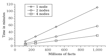
Figure 1: Win-not-win test for cyclic datasets. Time in minutes as a function of dataset size, for various numbers of nodes.

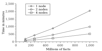
Figure 2: Win-not-win test for tree-structured datasets. Time in minutes as a function of dataset size, for various numbers of nodes.

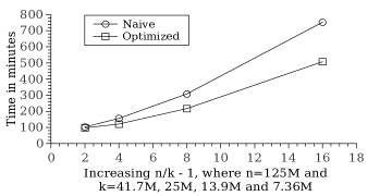
Figure 3: Transitive closure with negation test for chain-structured datasets. Time in minutes for increasing $\lceil n/k\rceil~{}-~{}1$, comparing naive and optimized WFS fixpoint calculation.

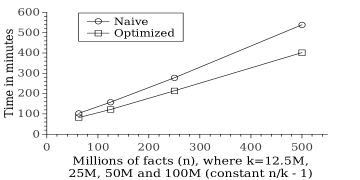
Figure 4: Transitive closure with negation test for chain-structured datasets. Time in minutes for constant $\lceil n/k\rceil~{}-~{}1$, comparing naive and optimized WFS fixpoint calculation.

6 Conclusion and Future Work

In this paper, we studied the feasibility of computing the well-founded semantics, while allowing recursion through negation, over large amounts of data. In particular, we proposed a parallel approach based on the MapReduce framework, ran experiments for various rule sets and data sizes, and showed the performance speedup coming from the optimized implementation when compared to a naive implementation. Our experimental results indicate that this method can be applied to billions of facts.

In future work, we plan to study more complex knowledge representation methods including Answer-Set programming (Gelfond (2008)), and RDF/S ontology evolution (Konstantinidis et al. (2008)) and repair (Roussakis et al. (2011)). We believe that these complex forms of reasoning do not fall under the category of “embarrassingly parallel” problems for which MapReduce is designed, and thus, a more complex computational model is required. Parallelization techniques such as OpenMP and Message Passing Interface (MPI) may provide higher degree of flexibility than the MapReduce framework, giving the opportunity to overcome arising limitations. In fact, in Answer-Set programming, the system claspar (Gebser et al. (2011)) uses MPI, but it needs a preliminary grounding step, as it accepts only ground or propositional programs. (Perri et al. (2013)) uses POSIX threads on shared memory for parallelized grounding. Combining these two approaches and making them more data-driven would be an interesting challenge.

Appendix A MapReduce algorithms

In the appendix, we include the algorithms that are used in the running examples of this paper. More specifically, Algorithm 3 refers to the wordcount example in Section 2.1.

1:map(Long key, String value): $\triangleright$ key: position in document

2:for all word w $\in$ value do $\triangleright$ value: document line

3:     emit(w, “1”);

4:end for

5:

6:reduce(String key, Iterator values): $\triangleright$ key: a word

7:int count = 0; $\triangleright$ values: list of counts

8:for all value $\in$ values do

9:     count += parseInt(value);

10:end for

11:emit(key, count);

Algorithm 3 Wordcount example

In Section 3.1 we described the calculation of the positive goal by applying a single join following Algorithm 4.

1:map(Long key, String value): $\triangleright$ key: position in document (irrelevant)

2:if value.predicate == “a” then $\triangleright$ value: document line (literal in I)

3:     emit(value.Z,{value.predicate,value.X});

4:else if value.predicate == “b” then

5:     emit(value.Z,{value.predicate,value.Y});

6:end if

7:

8:reduce(String key, Iterator values): $\triangleright$ key: matching argument

9:List a_List = $\emptyset$, b_List = $\emptyset$; $\triangleright$ values: literals in I for matching

10:for all value $\in$ values do

11:     if value.predicate == “a” then

12:         a_List.add(value.X);

13:     else if value.predicate == “b” then

14:         b_List.add(value.Y);

15:     end if

16:end for

17:for all a $\in$ a_List do

18:     for all b $\in$ b_List do

19:         emit(“ab(a.X,key.Z,b.Y)”,“”);

20:     end for

21:end for

Algorithm 4 Single join

Although we mentioned, in Section 3.1, that duplicate elimination should take place as soon as possible in order to minimize overhead, the description of the algorithm was deferred to this appendix. Duplicate elimination can be performed as described in Algorithm 5. Practically, the $Map$ function emits every inferred literal as the key, with an empty value. The MapReduce framework performs grouping/sorting resulting in one group (of duplicates) for each unique literal. Each group of duplicates consists of the unique literal as the key and a set of empty values (with values being eventually ignored). The actual duplicate elimination takes place during the reduce phase since for each group of duplicates, we emit the (unique) inferred literal once, using the key, while ignoring the values.

1:map(Long key, String value): $\triangleright$ key: position in document (irrelevant)

2:emit(value, “”); $\triangleright$ value: document line (inferred literal)

3:

4:reduce(String key, Iterator values): $\triangleright$ key: inferred literal

5:emit(key, “”); $\triangleright$ values: empty values (not used)

Algorithm 5 Duplicate elimination

Finally, the calculation of the final goal as described in Section 3.2 follows Algorithm 6.

1:map(Long key, String value): $\triangleright$ key: position in document (irrelevant)

2:if value.predicate == “ab” then $\triangleright$ value: document line (literal)

3:     emit({value.X,value.Z},{value.predicate,value.Y});

4:else if value.predicate == “c” then

5:     emit({value.X,value.Z},value.predicate);

6:end if

7:

8:reduce(String key, Iterator values): $\triangleright$ key: matching argument

9:List ab_List = $\emptyset$; $\triangleright$ values: literals for matching

10:for all value $\in$ values do

11:     if value.predicate == “ab” then

12:         ab_List.add(value.Y);

13:     else if value.predicate == “c” then

14:         return ; $\triangleright$ matched by predicate c

15:     end if

16:end for

17:for all ab $\in$ ab_List do

18:     emit(“abc(key.X,key.Z,ab.Y)”,“”);

19:end for

Algorithm 6 Anti-join

References

- Abiteboul et al. (1995) Abiteboul, S., Hull, R., and Vianu, V. 1995. Foundations of Databases. Addison-Wesley.
- Afrati and Ullman (2010) Afrati, F. N. and Ullman, J. D. 2010. Optimizing joins in a map-reduce environment. In EDBT, I. Manolescu, S. Spaccapietra, J. Teubner, M. Kitsuregawa, A. Léger, F. Naumann, A. Ailamaki, and F. Özcan, Eds. ACM International Conference Proceeding Series, vol. 426. ACM, 99–110.
- Brass et al. (2001) Brass, S., Dix, J., Freitag, B., and Zukowski, U. 2001. Transformation-based bottom-up computation of the well-founded model. Theory and Practice of Logic Programming 1, 5, 497–538.
- Cluet and Moerkotte (1994) Cluet, S. and Moerkotte, G. 1994. Classification and optimization of nested queries in object bases. Tech. rep.
- Dean and Ghemawat (2004) Dean, J. and Ghemawat, S. 2004. MapReduce: simplified data processing on large clusters. In Proceedings of the 6th conference on Symposium on Opearting Systems Design & Implementation - Volume 6. USENIX Association, Berkeley, CA, USA, 10–10.
- Fensel et al. (2008) Fensel, D., van Harmelen, F., Andersson, B., Brennan, P., Cunningham, H., Valle, E. D., Fischer, F., Huang, Z., Kiryakov, A., il Lee, T. K., Schooler, L., Tresp, V., Wesner, S., Witbrock, M., and Zhong, N. 2008. Towards LarKC: A Platform for Web-Scale Reasoning. In ICSC. 524–529.
- Gebser et al. (2011) Gebser, M., Kaminski, R., Kaufmann, B., Schaub, T., and Schnor, B. 2011. Cluster-based asp solving with claspar. In Logic Programming and Nonmonotonic Reasoning - 11th International Conference, LPNMR 2011, Vancouver, Canada, May 16-19, 2011. Proceedings, J. P. Delgrande and W. Faber, Eds. Lecture Notes in Computer Science, vol. 6645. 364–369.
- Gelder et al. (1991) Gelder, A. V., Ross, K. A., and Schlipf, J. S. 1991. The well-founded semantics for general logic programs. J. ACM 38, 3, 620–650.
- Gelfond (2008) Gelfond, M. 2008. Chapter 7 answer sets. In Handbook of Knowledge Representation, V. L. F. van Harmelen and B. Porter, Eds. Foundations of Artificial Intelligence, vol. 3. Elsevier, 285–316.
- Goodman et al. (2011) Goodman, E. L., Jimenez, E., Mizell, D., Al-Saffar, S., Adolf, B., and Haglin, D. J. 2011. High-performance computing applied to semantic databases. In ESWC (2), G. Antoniou, M. Grobelnik, E. P. B. Simperl, B. Parsia, D. Plexousakis, P. D. Leenheer, and J. Z. Pan, Eds. Lecture Notes in Computer Science, vol. 6644. Springer, 31–45.
- Konstantinidis et al. (2008) Konstantinidis, G., Flouris, G., Antoniou, G., and Christophides, V. 2008. A Formal Approach for RDF/S Ontology Evolution. In ECAI, M. Ghallab, C. D. Spyropoulos, N. Fakotakis, and N. M. Avouris, Eds. Frontiers in Artificial Intelligence and Applications, vol. 178. IOS Press, 70–74.
- Kotoulas et al. (2010) Kotoulas, S., Oren, E., and van Harmelen, F. 2010. Mind the data skew: distributed inferencing by speeddating in elastic regions. In WWW, M. Rappa, P. Jones, J. Freire, and S. Chakrabarti, Eds. ACM, 531–540.
- Liang et al. (2009) Liang, S., Fodor, P., Wan, H., and Kifer, M. 2009. Openrulebench: an analysis of the performance of rule engines. In Proceedings of the 18th international conference on World wide web. WWW ’09. ACM, New York, NY, USA, 601–610.
- Liu et al. (2011) Liu, C., Qi, G., Wang, H., and Yu, Y. 2011. Large scale fuzzy pD* reasoning using mapreduce. In Proceedings of the 10th international conference on The semantic web - Volume Part I. ISWC’11. Springer-Verlag, Berlin, Heidelberg, 405–420.
- Liu et al. (2012) Liu, C., Qi, G., Wang, H., and Yu, Y. 2012. Reasoning with Large Scale Ontologies in fuzzy pD* Using MapReduce. IEEE Comp. Int. Mag. 7, 2, 54–66.
- Mutharaju et al. (2010) Mutharaju, R., Maier, F., and Hitzler, P. 2010. A MapReduce Algorithm for EL+. In Description Logics.
- Nicolas (1982) Nicolas, J.-M. 1982. Logic for improving integrity checking in relational data bases. Acta Informatica 18, 227–253.
- Oren et al. (2009) Oren, E., Kotoulas, S., Anadiotis, G., Siebes, R., ten Teije, A., and van Harmelen, F. 2009. Marvin: Distributed reasoning over large-scale Semantic Web data. J. Web Sem. 7, 4, 305–316.
- Perri et al. (2013) Perri, S., Ricca, F., and Sirianni, M. 2013. Parallel instantiation of asp programs: techniques and experiments. Theory and Practice of Logic Programming 13, 2, 253–278.
- Roussakis et al. (2011) Roussakis, Y., Flouris, G., and Christophides, V. 2011. Declarative Repairing Policies for Curated KBs. In HDMS.
- Soma and Prasanna (2008) Soma, R. and Prasanna, V. K. 2008. Parallel Inferencing for OWL Knowledge Bases. In ICPP. IEEE Computer Society, 75–82.
- Tachmazidis and Antoniou (2013) Tachmazidis, I. and Antoniou, G. 2013. Computing the Stratified Semantics of Logic Programs over Big Data through Mass Parallelization. In RuleML, L. Morgenstern, P. S. Stefaneas, F. Lévy, A. Wyner, and A. Paschke, Eds. Lecture Notes in Computer Science, vol. 8035. Springer, 188–202.
- Tachmazidis et al. (2012) Tachmazidis, I., Antoniou, G., Flouris, G., and Kotoulas, S. 2012. Towards Parallel Nonmonotonic Reasoning with Billions of Facts. In KR, G. Brewka, T. Eiter, and S. A. McIlraith, Eds. AAAI Press.
- Tachmazidis et al. (2012) Tachmazidis, I., Antoniou, G., Flouris, G., Kotoulas, S., and McCluskey, L. 2012. Large-scale Parallel Stratified Defeasible Reasoning. In ECAI, L. D. Raedt, C. Bessière, D. Dubois, P. Doherty, P. Frasconi, F. Heintz, and P. J. F. Lucas, Eds. Frontiers in Artificial Intelligence and Applications, vol. 242. IOS Press, 738–743.
- Urbani et al. (2012) Urbani, J., Kotoulas, S., Massen, J., van Harmelen, F., and Bal, H. 2012. Webpie: A Web-scale parallel inference engine using MapReduce. Web Semantics: Science, Services and Agents on the World Wide Web 10, 0.