Positions of equilibrium points for dust particles in the circular restricted three-body problem with radiation

Abstract

For a body with negligible mass moving in the gravitational field of a star and one planet in a circular orbit (the circular restricted three-body problem) five equilibrium points exist and are known as the Lagrangian points. The positions of the Lagrangian points are not valid for dust particles because in the derivation of the Lagrangian points is assumed that no other forces beside the gravitation act on the body with negligible mass. Here we determined positions of the equilibrium points for the dust particles in the circular restricted three-body problem with radiation. The equilibrium points are located on curves connecting the Lagrangian points in the circular restricted three-body problem. The equilibrium points for Jupiter are distributed in large interval of heliocentric distances due to its large mass. The equilibrium points for the Earth explain a cloud of dust particles trailing the Earth observed with the Spitzer Space Telescope. The dust particles moving in the equilibrium points are distributed in interplanetary space according to their properties.

1 Introduction

Three bodies with masses moving under the action of their mutual Newtonian gravitation constitute the three-body problem in celestial mechanics. When one body has negligible mass with respect to the remaining two, we have the framework of the restricted three-body problem. The body with negligible mass does not influence the motion of the remaining two bodies, but its motion is determined by both of them. If the remaining two bodies orbit around their center of mass in circles, then the gravitational problem is called the circular restricted three-body problem (CR3BP). In the CR3BP the body with negligible mass can remain stationary in a reference frame rotating with the remaining two bodies around their center of mass. The stationary location of the body with negligible mass in the rotating frame is called the equilibrium point. The body with negligible mass located in the equilibrium point moves in a circular orbit with a constant speed in an inertial reference associated with center of mass of the two heavier bodies. Mutual distances of all three bodies are constant. Five such equilibrium points exist in the CR3BP. The points are called the Lagrangian points in honor of mathematician J. L. Lagrange. Three points are located on the line determined by two positions of the heavier bodies. The two remaining points create two equilateral triangles with the line connecting the two heavier bodies as a common base. Depending on the mass ratio of the two heavier bodies the points in the equilateral triangles can be stable. In 1906 first asteroid named Achilles was discovered near the stable Lagrangian point of Jupiter and the Sun. Today known asteroids near these stable points form Trojan group.

Unlike larger bodies dust particles can be significantly affected by weak non-gravitational forces. The Lorentz force is only important for submicrometer particles (Dohnanyi, 1978; Leinert & Grün, 1990; Dermott et al., 2001). These particles have large ratio of $Q/m$ ($Q$ is the charge of the dust particle and $m$ is the mass of the dust particle). The collisions among the dust particles are important for particles of radii larger than hundred of micrometres, approximately (Grün et al., 1985; Dermott et al., 2001). The motion of micron-sized dust particles in the inner part of the Solar system is influenced beside the gravitation mainly by solar electromagnetic radiation and solar wind. Consequences of the electromagnetic radiation on the motion of the interplanetary dust particles were already discussed in Poynting (1904). Robertson (1937) using relativity theory derived the equation of motion of a perfectly absorbing and thermally equilibrated sphere in covariant form. On the basis of these works influence of the electromagnetic radiation on the motion of the spherical dust particle is usually called the Poynting–Roberson (PR) effect. The PR effect contains a radial radiation pressure term for which inclusion in the CR3BP is equivalent to inclusion of a less massive star in the CR3BP and this changes the positions of the Lagrangian equilibrium points if the radial radiation pressure term is considered. This was outlined by Colombo, Lautman & Shapiro (1966) and Schuerman (1980). They also studied the stability of the equilibrium points in the CR3BP with the PR effect. Murray (1994) systematically discussed the dynamical effect of general drag in the planar CR3BP. Liou, Zook & Jackson (1995) investigated the effect of the PR effect and the radial solar wind in the restricted three-body problem. However, some of aspects of the motion of the dust particles in the vicinity of their equilibrium points in the CR3BP with radiation are still unknown. In this work we use an improved derivation of the PR effect presented in Klačka et al. (2014), which followed results derived in Klačka (1992, 2004, 2009a, 2009b). The improved derivation take into account arbitrary optical properties of particle with material distributed in a spherically symmetric way. The improved derivation leads to the same result for the case considered in Robertson (1937). The relativistic derivation of the PR effect can be generalized also for the solar wind. This was done in Klačka et al. (2012).

2 Equilibrium points

Let us consider the motion of a dust particle in the vicinity of a star with one planet in a circular orbit. The star produces spherically symmetric electromagnetic radiation and stellar wind which will be taken into account. Since orbital speed of the star is slow (small radius of the orbit and small angular velocity), relativistic corrections caused by transformations from a frame associated with the center of mass of the star and the planet into the frame associated with the star can be neglected. The accelerations of the dust particle caused by the electromagnetic radiation and the stellar wind will be determined in a reference frame associated with the star using the theory of relativity to first order in $v^{\prime}/c$ ($v^{\prime}$ is the speed of the dust particle with respect to the star and $c$ is the speed of light), first order in $u^{\prime}/c$ ($u^{\prime}$ is the speed of the stellar wind with respect to the star), and first order in $v^{\prime}/u^{\prime}$. In this case the equation of motion of the dust particle in the reference frame associated with the star is

$$\frac{d^{2}\vec{r}}{dt^{2}}={} -\frac{GM_{1}}{r^{3}}\vec{r}-\frac{GM_{2}}{\left|\vec{r}_{3}-\vec{r}_{2}\right|^{3}}\left(\vec{r}_{3}-\vec{r}_{2}\right)+\frac{GM_{2}}{\left|\vec{r}_{1}-\vec{r}_{2}\right|^{3}}\left(\vec{r}_{1}-\vec{r}_{2}\right)+$$

$$+\beta\frac{GM_{1}}{r^{2}}\left[\left(1-\frac{\vec{v^{\prime}}\cdot\vec{e}_{\text{R}}}{c}\right)\vec{e}_{\text{R}}-\frac{\vec{v^{\prime}}}{c}\right]+\frac{\eta}{\bar{Q^{\prime}}_{\text{pr}}}\beta\frac{u^{\prime}}{c}\frac{GM_{1}}{r^{2}}\left[\left(1-\frac{\vec{v^{\prime}}\cdot\vec{e}_{\text{R}}}{u^{\prime}}\right)\vec{e}_{\text{R}}-\frac{\vec{v^{\prime}}}{u^{\prime}}\right]~{}.$$ (1)

The first three terms are caused by the Newton gravitation of the star and the planet and the last two terms are the PR effect (Klačka et al., 2014) and the radial stellar wind (Klačka et al., 2012). $\vec{r}_{i}$, $i$ $=$ 1, 2, 3, are, respectively, the positions vectors of the star, planet and particle determined with respect to the center of mass of the two heavier bodies. $\vec{v^{\prime}}$ is the velocity of the dust particle with respect to the star, $G$ is the gravitational constant, $M_{1}$ is the mass of the star, and $M_{2}$ is the mass of the planet. $\vec{r}$ $=$ $\vec{r}_{3}-\vec{r}_{1}$ is the position vector of the particle with respect to the star, $r$ $=$ $\left|\vec{r}\right|$ and $\vec{e}_{\text{R}}$ $=$ $\vec{r}/r$ is the unit vector directed from the star to the particle. The parameter $\beta$ is defined as the ratio between the electromagnetic radiation pressure force and the gravitational force between the star and the particle at rest with respect to the star

$$\beta=\frac{L_{\star}A^{\prime}\bar{Q^{\prime}}_{\text{pr}}}{4\pi cmGM_{1}}~{}.$$ (2)

Here, $L_{\star}$ is the stellar luminosity, $\bar{Q^{\prime}}_{\text{pr}}$ is the dimensionless efficiency factor for the radiation pressure determined in the proper frame of the particle and averaged over the stellar spectrum, $A^{\prime}$ is the geometrical cross-section of the spherical particle determined in the proper frame of the particle, $c$ is the speed of light, and $m$ is the mass of the dust particle. The parameter $\eta$ describes the magnitude of acceleration caused by the radial stellar wind

$$\eta=\frac{4\pi r^{2}u^{\prime}}{L_{\star}}\sum_{i=1}^{N}n_{\text{sw}~{}i}m_{\text{sw}~{}i}c^{2}~{},$$ (3)

where $m_{\text{sw}~{}i}$ and $n_{\text{sw}~{}i}$, $i$ $=$ 1 to $N$, are the masses and concentrations of the stellar wind particles at a distance $r$ from the star ($u^{\prime}$ $=$ 450 km/s and $\eta$ $=$ 0.38 for the Sun, Klačka et al. 2012). To the given accuracy $\eta$ is the ratio of stellar wind energy to stellar electromagnetic radiation energy, both radiated per unit of time.

We assume that the mass of the particle is negligible with respect to the mass of star and also with respect to the mass of planet. Therefore, the Newton equations of motion of the two heavier bodies, only under the action of their mutual gravitational interaction, in the barycentric reference frame are

$$\frac{d^{2}\vec{r}_{1}}{dt^{2}} =-\frac{GM_{2}}{\left|\vec{r}_{1}-\vec{r}_{2}\right|^{3}}\left(\vec{r}_{1}-\vec{r}_{2}\right)~{},$$

$$\frac{d^{2}\vec{r}_{2}}{dt^{2}} =-\frac{GM_{1}}{\left|\vec{r}_{2}-\vec{r}_{1}\right|^{3}}\left(\vec{r}_{2}-\vec{r}_{1}\right)~{}.$$ (4)

In order to obtain the equation of motion of the dust particle in the barycentric reference frame we can use the following relation

$$\frac{d^{2}\vec{r}_{3}}{dt^{2}}=\frac{d^{2}\vec{r}}{dt^{2}}+\frac{d^{2}\vec{r}_{1}}{dt^{2}}~{}.$$ (5)

Eq. (5) with substituted Eq. (2) and the first of Eqs. (2) yields

$$\frac{d\vec{v}}{dt}={} -\frac{GM_{1}}{r^{3}}\vec{r}-\frac{GM_{2}}{\left|\vec{r}_{3}-\vec{r}_{2}\right|^{3}}\left(\vec{r}_{3}-\vec{r}_{2}\right)+\beta\frac{GM_{1}}{r^{2}}\left[\left(1-\frac{\vec{v^{\prime}}\cdot\vec{e}_{\text{R}}}{c}\right)\vec{e}_{\text{R}}-\frac{\vec{v^{\prime}}}{c}\right]+$$

$$+\frac{\eta}{\bar{Q^{\prime}}_{\text{pr}}}\beta\frac{u^{\prime}}{c}\frac{GM_{1}}{r^{2}}\left[\left(1-\frac{\vec{v^{\prime}}\cdot\vec{e}_{\text{R}}}{u^{\prime}}\right)\vec{e}_{\text{R}}-\frac{\vec{v^{\prime}}}{u^{\prime}}\right]~{},$$ (6)

where $\vec{v}$ is the velocity of the dust particle in the barycentric coordinate system. For stars similar to our Sun inequality $(\eta/\bar{Q}^{\prime}_{\text{pr}})(u^{\prime}/c)$ $\ll$ 1 holds and Eq. (2) can be simplified

$$\frac{d\vec{v}}{dt}=-\frac{GM_{1}\left(1-\beta\right)}{r^{3}}\vec{r}-\frac{GM_{2}}{\left|\vec{r}_{3}-\vec{r}_{2}\right|^{3}}\left(\vec{r}_{3}-\vec{r}_{2}\right)-\beta\frac{GM_{1}}{r^{2}}\left(1+\frac{\eta}{\bar{Q^{\prime}}_{\text{pr}}}\right)\left(\frac{\vec{v^{\prime}}\cdot\vec{e}_{\text{R}}}{c}\vec{e}_{\text{R}}+\frac{\vec{v^{\prime}}}{c}\right)~{}.$$ (7)

In next step we will assume that we have found an equilibrium point for the dust particle in a coordinate system rotating around the barycenter with an angular velocity $n$ equal to the mean motion of the two-body system. In the rotating coordinate system the dust particle located in the equilibrium remains stationary. In the barycentric coordinate system the dust particle located in the equilibrium point moves in a circular orbit with a constant speed. Coordinates in the barycentric system will be denoted by $x$, $y$ and $z$. The plane $xy$ in the chosen coordinate system coincides with the orbital plane of the star and the planet. The planet in the barycentric coordinate system moves counterclockwise when we look from the positive $z$-axis. Let actual coordinates of the equilibrium point in the barycentric system be $x$ and $y$. Then the velocity of the dust particle in the barycentric coordinate system is

$$\vec{v}=\left(-yn,~{}xn,~{}0\right)~{}.$$ (8)

Similarly for the star

$$\vec{v_{\text{S}}}=\left(-y_{1}n,~{}x_{1}n,~{}0\right)~{}.$$ (9)

For the velocity of the dust particle in the reference frame associated with the star we obtain

$$\vec{v^{\prime}}=\vec{v}-\vec{v_{\text{S}}}=\left(-\left(y-y_{1}\right)n,~{}\left(x-x_{1}\right)n,~{}0\right)~{}.$$ (10)

For the unit vector $\vec{e}_{\text{R}}$ directed from the star to the particle we obtain

$$\vec{e}_{\text{R}}=\frac{\vec{r}_{3}-\vec{r}_{1}}{r}=\frac{1}{r}\left(x-x_{1},~{}y-y_{1},~{}z\right)~{}.$$ (11)

The scalar product in Eq. (7) on the basis of Eq. (10) and Eq. (11) is

$$\vec{v^{\prime}}\cdot\vec{e}_{\text{R}}=0~{}.$$ (12)

Hence, only the term proportional to $\vec{v^{\prime}}$ in the acceleration caused by the non-gravitational effects remains and for the dust particle in the equilibrium point we have (Eq. 7)

$$\frac{d\vec{v}}{dt}=-\frac{GM_{1}\left(1-\beta\right)}{r^{3}}\vec{r}-\frac{GM_{2}}{\left|\vec{r}_{3}-\vec{r}_{2}\right|^{3}}\left(\vec{r}_{3}-\vec{r}_{2}\right)-\beta\frac{GM_{1}}{cr^{2}}\left(1+\frac{\eta}{\bar{Q^{\prime}}_{\text{pr}}}\right)\vec{v^{\prime}}~{}.$$ (13)

For the equilibrium points located out of the $xy$ plane we obtain from the $z$-component of Eq. (13)

$$\frac{GM_{1}\left(1-\beta\right)}{r^{3}}+\frac{GM_{2}}{\left|\vec{r}_{3}-\vec{r}_{2}\right|^{3}}=0~{}.$$ (14)

This equation does not have any solution for the dust particles with $\beta$ $<$ 1 (for discussion of the out of plane equilibrium points with $\beta$ $>$ 1 see Colombo et al. 1966). In what follows we will consider only the equilibrium points located in the $xy$ plane.

Introducing the transformation between the barycentric coordinate system and the system rotating around the barycenter with the angular velocity $n$

$$x =x_{\text{R}}\cos nt-y_{\text{R}}\sin nt~{},$$

$$y =x_{\text{R}}\sin nt+y_{\text{R}}\cos nt$$ (15)

Eq. (13) can be written in the following form

$$\frac{dx_{\text{R}}^{2}}{dt^{2}}-2n\frac{dy_{\text{R}}}{dt}-n^{2}x_{\text{R}}={} -\frac{GM_{1}\left(1-\beta\right)}{r^{3}}\left(x_{\text{R}}-x_{\text{1R}}\right)-\frac{GM_{2}}{\left|\vec{r}_{3}-\vec{r}_{2}\right|^{3}}\left(x_{\text{R}}-x_{\text{2R}}\right)$$

$$+\beta\frac{GM_{1}}{cr^{2}}\left(1+\frac{\eta}{\bar{Q^{\prime}}_{\text{pr}}}\right)ny_{\text{R}}~{},$$

$$\frac{dy_{\text{R}}^{2}}{dt^{2}}+2n\frac{dx_{\text{R}}}{dt}-n^{2}y_{\text{R}}={} -\frac{GM_{1}\left(1-\beta\right)}{r^{3}}y_{\text{R}}-\frac{GM_{2}}{\left|\vec{r}_{3}-\vec{r}_{2}\right|^{3}}y_{\text{R}}$$

$$-\beta\frac{GM_{1}}{cr^{2}}\left(1+\frac{\eta}{\bar{Q^{\prime}}_{\text{pr}}}\right)n\left(x_{\text{R}}-x_{\text{1R}}\right)~{},$$ (16)

where we have assumed that $y_{\text{1R}}$ $=$ $y_{\text{2R}}$ $=$ 0 holds for the star and the planet. For an equilibrium point the time derivatives of the coordinates in the rotating reference frame are zero and we obtain

$$n^{2}x_{\text{R}} =\frac{GM_{1}\left(1-\beta\right)}{r^{3}}\left(x_{\text{R}}-x_{\text{1R}}\right)+\frac{GM_{2}}{\left|\vec{r}_{3}-\vec{r}_{2}\right|^{3}}\left(x_{\text{R}}-x_{\text{2R}}\right)-\beta\frac{GM_{1}}{cr^{2}}\left(1+\frac{\eta}{\bar{Q^{\prime}}_{\text{pr}}}\right)ny_{\text{R}}~{},$$

$$n^{2}y_{\text{R}} =\frac{GM_{1}\left(1-\beta\right)}{r^{3}}y_{\text{R}}+\frac{GM_{2}}{\left|\vec{r}_{3}-\vec{r}_{2}\right|^{3}}y_{\text{R}}+\beta\frac{GM_{1}}{cr^{2}}\left(1+\frac{\eta}{\bar{Q^{\prime}}_{\text{pr}}}\right)n\left(x_{\text{R}}-x_{\text{1R}}\right)~{}.$$ (17)

2.1 Equilibrium points without velocity terms

Equations (2) without the radiation terms resulting from the dependence of the acceleration in Eq. (7) on the relative velocity of the dust particle with respect to the star is not real. However, equilibrium points obtained from this equations can be used as first approximation during determination of more real positions of the equilibrium points. This is caused by the fact that from all terms in the acceleration caused by the radiation the radial term not depending on the relative velocity is dominant. The other terms are proportional to a ratio of a component of the relative velocity and the speed of light. By using this approximation we also assume that the terms resulting from the dependence on the relative velocity of the dust particle with respect to the star in Eqs. (2) can be neglected in comparison with the terms caused by the gravitational force of the planet. Positions of the equilibrium points for the system given by Eq. (2) without velocity terms are determined by

$$x_{\text{R}}n^{2} =\frac{GM_{1}\left(1-\beta\right)}{r^{3}}\left(x_{\text{R}}-x_{\text{1R}}\right)+\frac{GM_{2}}{\left|\vec{r}_{3}-\vec{r}_{2}\right|^{3}}\left(x_{\text{R}}-x_{\text{2R}}\right)~{},$$

$$y_{\text{R}}n^{2} =\frac{GM_{1}\left(1-\beta\right)}{r^{3}}y_{\text{R}}+\frac{GM_{2}}{\left|\vec{r}_{3}-\vec{r}_{2}\right|^{3}}y_{\text{R}}~{}.$$ (18)

This system with $\beta$ $=$ 0 is the system which determines positions of the Lagrangian points in the circular restricted three-body problem. From the second equation we obtain two possibilities one with $y_{\text{R}}$ $=$ 0 and one with

$$n^{2}=\frac{GM_{1}\left(1-\beta\right)}{r^{3}}+\frac{GM_{2}}{\left|\vec{r}_{3}-\vec{r}_{2}\right|^{3}}~{}.$$ (19)

From the second Kepler’s law we have

$$n^{2}=\frac{G\left(M_{1}+M_{2}\right)}{a_{\text{P}}^{3}}~{},$$ (20)

where $a_{\text{P}}$ is the semimajor axis of the planet.

2.1.1 Analogy with the Lagrangian points $L_{4}$ and $L_{5}$

In the $x_{\text{P}}y_{\text{P}}$ plane only one distance from the star and one from the planet fulfills the condition Eq. (19) for a given $\beta$. The solution is

$$r =a_{\text{P}}\left(1-\beta\right)^{1/3}~{},$$

$$\left|\vec{r}_{3}-\vec{r}_{2}\right| =a_{\text{P}}~{}.$$ (21)

Coordinates of the points analogous to the Lagrangian points $L_{4}$ and $L_{5}$ are given by common points of the two circles given by Eqs. (2.1.1)

$$x_{\text{L}} =\frac{a_{\text{P}}\left[\left(1-\beta\right)^{2/3}-1\right]+x_{\text{1R}}+x_{\text{2R}}}{2}~{},$$

$$y_{\text{L}}^{2} =a_{\text{P}}^{2}\left\{1-\left[1-\frac{\left(1-\beta\right)^{2/3}}{2}\right]^{2}\right\}~{}.$$ (22)

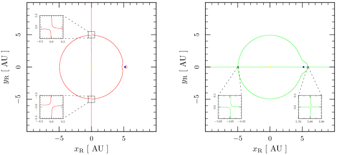
Figure 1: Calculated points in the $x_{\text{R}}y_{\text{R}}$ plane which fulfill the first (left) and the second (right) equation in the system of equations given by Eqs. (2). The equations are solved for a dust particle with radius $R$ $=$ 4 $\mu$m, density $\varrho$ $=$ 1 g/cm³, and $\bar{Q}^{\prime}_{\text{pr}}$ $=$ 1 in the system with Jupiter in a circular orbit around the radiating Sun.

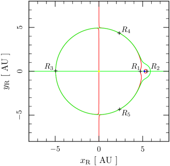
Figure 2: The equilibrium points obtained from the solution of Eqs. (2) depicted in Fig. 1. The system consists of Jupiter in a circular orbit around the Sun and a dust particle with radius $R$ $=$ 4 $\mu$m, mass density $\varrho$ $=$ 1 g/cm³, and $\bar{Q}^{\prime}_{\text{pr}}$ $=$ 1. We must note that the point $R_{2}$ is inside Jupiter’s shadow for the real Jupiter.

2.1.2 Analogy with the Lagrangian points $L_{1}$, $L_{2}$ and $L_{3}$

The condition $y_{\text{R}}$ $=$ 0 for a given $\beta$ is fulfilled by three different $x_{\text{R}}$ determined by the first equation in Eqs. (2.1). For $x_{\text{1R}}$ and $x_{\text{2R}}$ we have from the two-body problem

$$x_{\text{1R}} =-\frac{M_{2}a_{\text{P}}}{M_{1}+M_{2}}~{},$$

$$x_{\text{2R}}-x_{\text{1R}} =a_{\text{P}}~{}.$$ (23)

When we look from the planet, then for the point before the star we obtain

$$\frac{M_{\text{2}}}{M_{\text{1}}}=\frac{\left(1-\beta\right)a_{\text{P}}^{3}-\left(a_{\text{P}}-r_{\text{P}}\right)^{3}}{\left(a_{\text{P}}-r_{\text{P}}\right)^{2}\left(a_{\text{P}}^{3}-r_{\text{P}}^{3}\right)}r_{\text{P}}^{2}~{},$$ (24)

where $r_{\text{P}}$ is the distance of the point from the planet. This point is analogous to the Lagrangian point $L_{1}$. The equilibrium point analogous to the Lagrangian point $L_{2}$ is located in the opposite direction from the planet. From the first equation in Eqs. (2.1) we have

$$\frac{M_{\text{2}}}{M_{\text{1}}}=\frac{\left(1-\beta\right)a_{\text{P}}^{3}-\left(a_{\text{P}}+r_{\text{P}}\right)^{3}}{\left(a_{\text{P}}+r_{\text{P}}\right)^{2}\left(r_{\text{P}}^{3}-a_{\text{P}}^{3}\right)}r_{\text{P}}^{2}~{}.$$ (25)

Finally, the point analogous to the Lagrangian point $L_{3}$ is located behind the star with

$$\frac{M_{\text{2}}}{M_{\text{1}}}=\frac{\left(1-\beta\right)a_{\text{P}}^{3}+\left(a_{\text{P}}-r_{\text{P}}\right)^{3}}{\left(a_{\text{P}}-r_{\text{P}}\right)^{2}\left(r_{\text{P}}^{3}-a_{\text{P}}^{3}\right)}r_{\text{P}}^{2}~{}.$$ (26)

Coordinates of the points are $x_{\text{L}}$ $=$ $x_{\text{2R}}$ $-$ $r_{\text{P}}$, $x_{\text{L}}$ $=$ $x_{\text{2R}}$ $+$ $r_{\text{P}}$, and $x_{\text{L}}$ $=$ $x_{\text{2R}}$ $-$ $r_{\text{P}}$ with $y_{\text{L}}$ $=$ 0, where $r_{\text{P}}$ has to be determined by Eq. (24), (25), and (26), respectively.

2.2 Equilibrium points with velocity terms

If are the velocity terms in the acceleration caused by the radiation taken into account, then Eqs. (2) determine positions of the equilibrium points exactly. One solution of Eqs. (2) is shown in Fig. 1. We assumed that the system consists of Jupiter in a circular orbit around the Sun and a dust particle with radius $R$ $=$ 4 $\mu$m, mass density $\varrho$ $=$ 1 g/cm³, and $\bar{Q}^{\prime}_{\text{pr}}$ $=$ 1. The left part of the figure corresponds to the first equation in Eqs. (2) and the right part of the figure corresponds to the second equation in Eqs. (2). The solution of the first equation is formed by three separated curves which do not intersect each other. The solution of the second equation is formed by a single curve without intersection. Theoretically, intersections of the curve corresponding to the solution of the second equation exist for no radiation case ($\beta$ $=$ 0) because $y_{\text{R}}$ $=$ 0 is always one solution. The equilibrium points can be obtained as common points of the curves were both equations in Eqs. (2) hold at once. The equilibrium points determined by the common points of the curves in Fig. 1 are depicted in Fig. 2. Five equilibrium points exist in this case. This numerical method always allows the determination of the positions of the equilibrium points.

Figures 1 and 2 show that the solutions of the system of equations in Eqs. (2) have relative complicated behavior. We must have in mind that these figures hold only for a single value of $\beta$. In order to find the positions of the equilibrium points analytically and overcome the relatively complicated behavior of solutions of Eqs. (2) we developed an analytical method which will be now presented. Suppose that the terms resulting from the dependence of acceleration of the dust particle on the relative velocity are small in comparison with all other terms in Eqs. (2). In this case the positions of the equilibrium points will be approximately determined by the theory presented in Section 2.1. The last two terms in Eqs. (2) will create only a shift from the positions analogous to the Lagrangian points. We will denote this shift as $\Delta x_{\text{R}}$ and $\Delta y_{\text{R}}$. The position analogous to the Lagrangian points will denoted by $x_{\text{L}}$ and $y_{\text{L}}$. Using a Taylor series for functions with two variables to first order

$$f\left(x_{\text{R}},y_{\text{R}}\right)\approx f\left(x_{\text{L}},y_{\text{L}}\right)+\left(\frac{\partial f}{\partial x_{\text{R}}}\right)_{x_{\text{L}},y_{\text{L}}}\left(x_{\text{R}}-x_{\text{L}}\right)+\left(\frac{\partial f}{\partial y_{\text{R}}}\right)_{x_{\text{L}},y_{\text{L}}}\left(y_{\text{R}}-y_{\text{L}}\right)~{}.$$ (27)

we can approximate the expressions with the distances in Eqs. (2)

$$\frac{1}{\left|\vec{r}_{3}-\vec{r}_{1}\right|^{3}} \approx\frac{1}{r_{\text{1L}}^{3}}+\frac{3\left(x_{\text{1R}}-x_{\text{L}}\right)}{r_{\text{1L}}^{5}}\Delta x_{\text{R}}-\frac{3y_{\text{L}}}{r_{\text{1L}}^{5}}\Delta y_{\text{R}}~{},$$

$$\frac{1}{\left|\vec{r}_{3}-\vec{r}_{1}\right|^{2}} \approx\frac{1}{r_{\text{1L}}^{2}}+\frac{2\left(x_{\text{1R}}-x_{\text{L}}\right)}{r_{\text{1L}}^{4}}\Delta x_{\text{R}}-\frac{2y_{\text{L}}}{r_{\text{1L}}^{4}}\Delta y_{\text{R}}~{},$$

$$\frac{1}{\left|\vec{r}_{3}-\vec{r}_{2}\right|^{3}} \approx\frac{1}{r_{\text{2L}}^{3}}+\frac{3\left(x_{\text{2R}}-x_{\text{L}}\right)}{r_{\text{2L}}^{5}}\Delta x_{\text{R}}-\frac{3y_{\text{L}}}{r_{\text{2L}}^{5}}\Delta y_{\text{R}}~{},$$ (28)

where

$$r_{\text{1L}} =\sqrt{\left(x_{\text{1R}}-x_{\text{L}}\right)^{2}+y_{\text{L}}^{2}}~{},$$

$$r_{\text{2L}} =\sqrt{\left(x_{\text{2R}}-x_{\text{L}}\right)^{2}+y_{\text{L}}^{2}}~{}.$$ (29)

Substitution of Eqs. (2.2) into Eqs. (2) leads to the following system of equations with two unknowns $\Delta x_{\text{R}}$ and $\Delta y_{\text{R}}$

$$a_{11}\Delta x_{\text{R}}+a_{12}\Delta y_{\text{R}}+b_{1}=0~{},$$

$$a_{21}\Delta x_{\text{R}}+a_{22}\Delta y_{\text{R}}+b_{2}=0~{},$$ (30)

where

$$a_{11}={} 2n^{2}+\frac{GM_{1}\left(1-\beta\right)}{r_{\text{1L}}^{3}}+\frac{GM_{2}}{r_{\text{2L}}^{3}}-a_{22}~{},$$

$$a_{12}={} \frac{3GM_{1}\left(1-\beta\right)}{r_{\text{1L}}^{5}}\left(x_{\text{L}}-x_{\text{1R}}\right)y_{\text{L}}+\frac{3GM_{2}}{r_{\text{2L}}^{5}}\left(x_{\text{L}}-x_{\text{2R}}\right)y_{\text{L}}$$

$$+\frac{\beta GM_{1}}{c}\left(1+\frac{\eta}{\bar{Q^{\prime}}_{\text{pr}}}\right)n\left(\frac{1}{r_{\text{1L}}^{2}}-\frac{2y_{\text{L}}^{2}}{r_{\text{1L}}^{4}}\right)~{},$$

$$a_{21}={} a_{12}~{},$$

$$a_{22}={} n^{2}-\frac{GM_{1}\left(1-\beta\right)}{r_{\text{1L}}^{3}}-\frac{GM_{2}}{r_{\text{2L}}^{3}}+\frac{3GM_{1}\left(1-\beta\right)}{r_{\text{1L}}^{5}}y_{\text{L}}^{2}$$

$$+\frac{3GM_{2}}{r_{\text{2L}}^{5}}y_{\text{L}}^{2}+\frac{2\beta GM_{1}}{c}\left(1+\frac{\eta}{\bar{Q^{\prime}}_{\text{pr}}}\right)n\frac{\left(x_{\text{L}}-x_{\text{1R}}\right)y_{\text{L}}}{r_{\text{1L}}^{4}}~{},$$

$$b_{1}={} \frac{\beta GM_{1}}{c}\left(1+\frac{\eta}{\bar{Q^{\prime}}_{\text{pr}}}\right)n\frac{y_{\text{L}}}{r_{\text{1L}}^{2}}~{},$$

$$b_{2}={} -\frac{\beta GM_{1}}{c}\left(1+\frac{\eta}{\bar{Q^{\prime}}_{\text{pr}}}\right)n\frac{x_{\text{L}}-x_{\text{1R}}}{r_{\text{1L}}^{2}}~{}.$$ (31)

Eqs. (2.2) and (2.2) enable to determine unknown shift from the points analogous to the Lagrangian points. The determination of the shift from the points analogous to $L_{4}$ and $L_{5}$ using Eqs. (2.2) can be simplified with identity

$$n^{2}=\frac{GM_{1}\left(1-\beta\right)}{r_{\text{1L}}^{3}}+\frac{GM_{2}}{r_{\text{2L}}^{3}}$$ (32)

and the substitution $y_{\text{L}}$ $=$ 0 simplify Eqs. (2.2) for the shift from the points analogous to $L_{1}$, $L_{2}$ and $L_{3}$.

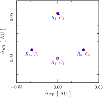
Figure 3: Calculated ($C$) and real ($R$) shifts of the positions of dust particle from the points analogous to the Lagrangian points in the CR3BP with radiation. The shifts are determined for the system solved in Fig. 1 and Fig. 2. The circles are used for the calculated positions, the triangles are used for the real positions and the star denotes the position of the points analogous to the Lagrangian points.

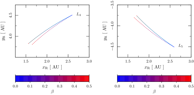
Figure 4: The positions of real equilibrium points (solid line) compared with the positions of equilibrium points calculated from Eqs. (2.2) (azure dashed line) and the positions of points analogous to the Lagrangian points (dotted line) for Jupiter in a circular orbit around the Sun and dust particles with $\beta$ $\in$ [0, 0.5] and $\bar{Q^{\prime}}_{\text{pr}}$ $=$ 1. Only the stable equilibrium points resulting from the points analogous to the Lagrangian points $L_{4}$ and $L_{5}$ are depicted.

Figure 3 shows the shifts of equilibrium points from positions analogous to the Lagrangian points determined using system of equation Eqs. (2.2) (circles) and the real shifts determined using the numerical solution of Eqs. (2) (triangles). The parameters of system are the same as for Fig. 1 and Fig. 2. As can be seen the positions of equilibrium points differ from the positions of points analogous to $L_{3}$, $L_{4}$ and $L_{5}$. The position of equilibrium point derived from the point analogous to $L_{1}$ is determined mainly by the gravitational influence of the planet in this case and thus its position is not significantly affected by the radiation terms depending on the relative velocity. The point analogous to $L_{2}$ is inside Jupiter’s shadow and is not shown.

Figure 4 shows the positions of the stable equilibrium points resulting from the points analogous to the Lagrangian points $L_{4}$ and $L_{5}$ in the system consisting of Jupiter in a circular orbit around the Sun, and the dust particles with $\beta$ $\in$ [0, 0.5] and $\bar{Q^{\prime}}_{\text{pr}}$ $=$ 1. The positions of equilibrium points determined from the numerical solution of Eqs. (2) (solid line) are compared with the positions of equilibrium points determined from Eqs. (2.2) (azure dashed line). The positions of points analogous to the Lagrangian points $L_{4}$ and $L_{5}$ are also shown (dotted line). In Fig. 4 we can see that the theory leading to the system of equations represented by Eqs. (2.2) is in an excellent agreement with the numerical solution of Eqs. (2) for the considered system.

Figure 5 shows complete set of the equilibrium points for Jupiter and the Sun. It is purely theoretical case in the CR3BP with included radiation. In Fig. 5 we can see that as $\beta$ increases from zero the equilibrium points emerge from the Lagrangian points. The Lagrangian points $L_{1}$ and $L_{5}$ are connected with a curve determined by locations of the equilibrium points. We will call such curves equilibrium branches or simply branches. Similarly the Lagrangian points $L_{3}$ and $L_{4}$ create an equilibrium branch.

In Murray (1994) the first branch is obtained between $L_{2}$ and $L_{5}$ and the second branch is obtained between $L_{3}$ and $L_{4}$. A method used in Murray (1994) does not eliminate dependence on $\beta$ in a resulting equation equivalent to Eq. (99) in Murray (1994) for the complete acceleration caused by the PR effect and the radial solar wind. If this method would be used for Eqs. (2), then the dependence on $\eta/\bar{Q^{\prime}}_{\text{pr}}$ would be eliminated. This leads to equilibrium points obtained for a given $\beta$ and all possible $\eta/\bar{Q^{\prime}}_{\text{pr}}$. This is not appropriate for a given star. Dependence on $\beta$ remains in the resulting equation due to the radiation term which does not depend on the relative velocity in Eq. (7). Moreover, the drag term considered in Murray (1994) depends on the velocity of the dust particle with respect to the center of mass of the two heavier bodies (compare Eqs. 93 and 121 in Murray 1994) and the PR effect give dependence on the relative velocity of the dust particle with respect to the star (Eq. 13). The dependence on the velocity of the dust particle with respect to the center of mass of the two-body system in the PR effect and the radial solar wind was also used in Liou et al. (1995). They numerically obtained positions for the equilibrium points for $\beta$ $\in$ {0, 0.1, 0.2, …, 0.9}. Their Fig. 2 at least qualitatively corresponds with the results presented in Fig. 5. However, from Fig. 2 in Liou et al. (1995) can not be determined which Lagrangian points are connected with equilibrium branches.

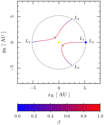
Figure 5: Complete set of the equilibrium points in the circular restricted three-body problem with radiation. Jupiter in a circular orbit around the Sun is taken into account. The Lagrangian points $L_{1}$ and $L_{5}$ create an equilibrium branch. Similarly as $L_{3}$ and $L_{4}$. Black lines perpendicular on the branches separate stable and unstable parts of the branches. Only the Lagrangian point $L_{2}$ is depicted behind Jupiter since the other equilibrium points resulting from $L_{2}$ are inside Jupiter’s shadow.

The stability of the equilibrium points can be verified directly from the numerical solution of the equation of motion (Eq. 7). A point which separates branches into stable and unstable parts exists on both branches in Fig. 5. The location of this separation point is depicted with a black line perpendicular on both branches. The separation point for $L_{1}$–$L_{5}$ branch is closer then 1 AU from the Sun. The separation point is the only equilibrium point on the $L_{1}$–$L_{5}$ branch for $\beta$ $\approx$ 0.9935. For larger values of $\beta$ no equilibrium point exists on the $L_{1}$–$L_{5}$ branch. The part of the branch $L_{1}$–$L_{5}$ from the Lagrangian point $L_{5}$ to the separation point is stable and the remaining part of the branch is unstable. Similarly for the branch $L_{3}$–$L_{4}$. The separation point on the $L_{3}$–$L_{4}$ branch is theoretically obtained for a dust particle with $\beta$ $\approx$ 0.9880. If the particle is initially near its equilibrium point on the stable part of a branch, then the particle will librate around the equilibrium point. The particle near its equilibrium point on the unstable part of the branch does not librate and its distance from the equilibrium point gradually increases. The libration around an equilibrium point on the stable part of branch is characterized with small increase of the maximal distance from the equilibrium point (libration amplitude) after one libration period. Therefore, the particles librating around the equilibrium points on the stable part of branch cannot remain in the libration and need to be replenished. The increase of libration amplitude (instability of the equilibrium points) can be derived analytically (see the comment after Eq. 34). As the particles librate time variations in the solar wind can also change the libration amplitude. A particle with $\beta$ $<$ 1 can move in a bound orbit after an ejection from a parent body. A particle with $\beta$ $>$ 1 escapes from the Solar system as $\beta$-meteoroid (Zook & Berg, 1975). We must note that for the particles with large $\beta$ (submicrometer particles) the Lorentz force cannot be always neglected in comparison with the PR effect and the radial solar wind (Dohnanyi, 1978; Leinert & Grün, 1990; Dermott et al., 2001). If the dust particle is already in the bound orbit, then the PR effect and the radial solar wind decrease the semimajor axis and eccentricity of the particle’s orbit (Wyatt & Whipple, 1950). Hence, the particle can get closer to circular orbits from larger values of semimajor axes. This processes can take place after the ejection of the dust particles from asteroids after mutual collisions or from comets during their approach to the Sun. The dust particles spiralling toward the Sun can get to the vicinity of the equilibrium points.

Figure 6 depicts locations of the equilibrium points for the Earth in the CR3BP with radiation. The black lines perpendicular to the equilibrium branches split the branches into stable and unstable parts in Fig. 6. Similarly to Fig. 5. Only the Lagrangian point $L_{2}$ is shown behind the Earth. The others equilibrium points resulting from the equilibrium near $L_{2}$ are partially in shadow cast by the Earth in the sunlight. The Lagrangian point $L_{2}$ is 0.0100 AU behind the Earth and full shadow of the real Earth extend to $\sim$0.0093 AU. These equilibrium points are also engulfed in the magnetosphere of the Earth. The magnetotail of the Earth can exceed to 0.067 AU.

A circumsolar dust ring close to Earth’s orbit was observed by satellites IRAS (Dermott et al., 1994) and COBE (Reach et al., 1995). The dust particles in this ring can comprise particles moving close to the equilibrium points of the CR3BP with radiation. If we take into account these particles, then the cloud trailing the Earth observed with the Spitzer Space Telescope (Reach, 2010) can be easily explained. The particles forming the cloud librate around of the equilibrium points on the stable part of branch $L_{1}$–$L_{5}$. Fig. 6 shows that the stable part of branch $L_{1}$–$L_{5}$ gets close to the Earth in the trailing direction. The position of the cloud trailing the Earth observed with the Spitzer Space Telescope is in an accordance with consequences of used accelerations for the Poynting–Robertson effect and the radial solar wind. The left plot in Fig. 7 shows a dust particle with $\beta$ $=$ 0.08 and $\bar{Q^{\prime}}_{\text{pr}}$ $=$ 1 during 200 years of the libration around its equilibrium point on the stable part of branch $L_{1}$–$L_{5}$. If this particle would be continually replenished with the same initial conditions, then all dust particles would form a ring near the Earth’s orbit depicted in the right plot of Fig. 7. As the libration amplitude increases the particles spread from the equilibrium point around the orbit and form the ring. Number density $n$ of the particles in the ring decreases with increasing circumferential distance from the initial libration closest to the equilibrium point. During conjunctions of a dust particle with Jupiter the gravitation of Jupiter can be comparable with acceleration caused by the solar radiation in the vicinity of the Earth’s orbit (see Appendix A2 in Colombo et al. 1966). We have found using the numerical solution of the equation of motion of the dust particle in a planar restricted four-body problem with radiation that the libration of the dust particle close to the Earth trailing direction is not affected by the gravitation of Jupiter.

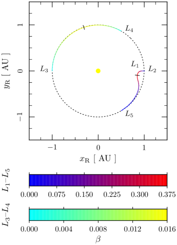
Figure 6: Positions of the equilibrium points of dust particles determined for the radiating Sun and the Earth in a circular orbit in the reference frame rotating with the Earth. The Lagrangian points $L_{1}$, $L_{3}$, $L_{4}$ $L_{5}$ are on the ends of equilibrium branches $L_{1}$–$L_{5}$ and $L_{3}$–$L_{4}$. The equilibrium points on the branch $L_{1}$–$L_{5}$ can be obtained for significantly smaller particles (larger $\beta$) than the smallest particle in the equilibrium point on the branch $L_{3}$–$L_{4}$. The stable part of branch $L_{1}$–$L_{5}$ gets close to the Earth in the trailing direction.

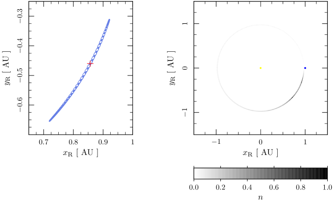
Figure 7: Left: Libration of a dust particle with $\beta$ $=$ 0.08 and $\bar{Q^{\prime}}_{\text{pr}}$ $=$ 1 around its equilibrium point on the stable part of the branch $L_{1}$–$L_{5}$. The position of the equilibrium is depicted with a red cross. Right: A ring formed by particles with the same properties and the initial conditions as the particle in the left plot. Number density $n$ of the chosen particle decreases with increasing circumferential distance from the initial libration depicted in the left plot.

The mean motion resonances (MMRs) occur when orbital periods of the particle and the Earth are in a ratio of natural numbers. If the dust particle is captured in an MMR, then variations of the semimajor axis are balanced by the resonant interaction with the planet’s gravitational field. The capture is only temporary (Gomes, 1995). The semimajor axis of the particle’s orbit in an MMR can be calculated using the third Kepler laws for the particle and the Earth. The result is

$$a_{\beta} =a_{\text{P}}\left(1-\beta\right)^{1/3}\left(\frac{T}{T_{\text{P}}}\right)^{2/3}\left(\frac{M_{1}}{M_{1}+M_{2}}\right)^{1/3}~{},$$

$$\frac{T}{T_{\text{P}}} =\frac{p}{q}~{},$$ (33)

where $T$ is the orbital period of the dust particle, $T_{\text{P}}$ is the orbital period of the Earth and $p$ and $q$ are two natural numbers. $p$ $>$ $q$ holds for the particle captured in an exterior MMR and $p$ $<$ $q$ holds for the capture in an interior MMR. The dust particles captured in the MMRs with the Earth undergo changes of their orbits caused by the solar radiation. From typical dust particles ($\beta$ $\ll$ 1) close to the Earth’s orbit can stay only the particles captured in MMRs with $p/q$ $\approx$ 1. The particles cannot be captured in the MMRs with $p/q$ $\approx$ 1 such a long time as particles captured in the MMRs given by a ratio of two small natural numbers due to a lack of encounters with the Earth. This holds for both the exterior and interior MMRs. Therefore, the most suitable resonance for the formation of the circumsolar dust ring close to Earth’s orbit is a special case, the resonance with $p/q$ $=$ 1/1 $=$ 1. This resonance has also long capture time in comparison with the capture times of resonances $p/q$ $\approx$ 1. Since the gravitation of the Sun is dominant for the dust particles in the equilibrium points approximately hold

$$r\approx a_{\text{P}}\left(1-\beta\right)^{1/3}~{},$$ (34)

where $r$ is the heliocentric distance. Similar equation can be obtained from Eq. (2.2) if we consider the dust particle in the 1/1 resonance in a circular orbit. The ring formed by the identical particles depicted in Fig. 7 represents one possible behavior of the dust particles captured into the 1/1 resonance with the Earth. The spherical dust particles captured in the 1/1 resonance in the planar CR3BP under the action of the PR effect and the radial stellar wind have an evolution of eccentricity which asymptotically decreases to a zero eccentricity (Pástor et al., 2009; Pástor, 2013). This feature enables using an application of adiabatic invariant theory presented in Gomes (1995) to prove that during the libration around an equilibrium point on the stable part of an equilibrium branch the libration amplitude must always increase. However, we can confirm result of Liou et al. (1995) that it is impossible for a dust particle to drift toward and get trapped in the 1/1 resonance when the dust particle is approaching under the PR effect and radial stellar wind. We found that such a capture is possible after close encounter with the planet.

Figures 4, 5 and 6 depicts that the equilibrium points are in interplanetary space distributed in space according to the properties of dust particles. This leads to applicable consequences. If the size and the mass of the dust particles could be measured during an interplanetary flight of a dust analyzing spacecraft, then parameter $\beta$ can be obtained for the measured particles (with the assumption $\bar{Q^{\prime}}_{\text{pr}}$ $=$ 1). For a spacecraft trajectory going through the equilibrium branches detection of the particles with the equilibrium properties should be more frequent. Such a measurement could test the applicability of the acceleration caused by the PR-effect and radial solar wind for the description of motion of the real interplanetary dust particles.

Interstellar medium atoms penetrate into the Solar System due to relative motion of the Solar System with respect to the interstellar medium. These approaching atoms form an interstellar gas flow. In the outer parts of the Solar system the acceleration of the dust particle caused by the interstellar gas flow cannot be neglected with respect to the accelerations caused by the PR effect and the radial solar wind (Pástor, Klačka & Kómar, 2011; Pástor, 2012). The interstellar gas flow significantly affects also the orbital evolution of the dust particles in the mean motion resonances (Pástor, 2013, 2014). Since the interstellar gas flow is monodirectional its implementation in the rotating reference frame in order to determine the positions of the equilibrium points is impossible. Hence, in the outer parts of the Solar system the equilibrium discussed in this paper cannot be obtained.

3 Conclusion

Equilibrium points exist for dust particles in the circular restricted three-body problem with radiation. Positions of the equilibrium points can be calculated with presented analytical method in the case when the terms resulting from the dependence of the acceleration of dust particle on the relative velocity between the particle and the star are small in comparison with all other terms in the acceleration. This assumption is not valid for the Earth due to its small mass. The Lagrangian points $L_{1}$ and $L_{5}$ are connected into an equilibrium branch for the dust particles. Similarly for the Lagrangian points $L_{3}$ and $L_{4}$. The equilibrium points of the Sun and Jupiter are located far from Jupiter’s orbit. The equilibrium points for the Earth explain the cloud of dust particles trailing the Earth. The dust particles moving in the equilibrium points are distributed in the interplanetary space according to their properties. This should have interesting applications in tests of the accelerations acting on the real interplanetary dust particles.

References

- Colombo et al. (1966) Colombo G., Lautman D. A., Shapiro I. I., 1966. The Earth’s Dust Belt: Fact or fiction? 2. Gravitational focusing and Jacobi capture. J. Geophys. Res. 71, 5705–5717.
- Dohnanyi (1978) Dohnanyi J. S., 1978. Particle dynamics. In: McDonnell J. A. M. (ed.), Cosmic Dust, Wiley-Interscience, Chichester, pp. 527–605.
- Dermott et al. (2001) Dermott S. F., Grogan K., Durda D. D., Jayaraman S., Kehoe T. J. J., Kortenkamp S. J., Wyatt M. C., 2001. Orbital evolution of interplanetary dust. In: Grün E., Gustafson B. A. S., Dermott S. F., Fechtig H. (eds.), Interplanetary Dust, Springer-Verlag, Berlin, pp. 569–639.
- Dermott et al. (1994) Dermott S. F., Jayaraman S., Xu Y. L., Gustafson B. A. S., Liou J.-C., 1994. A circumsolar ring of asteroidal dust in resonant lock with the Earth. Nature 369, 719–723.
- Gomes (1995) Gomes R. S., 1995. The effect of nonconservative forces on resonance lock: stability and instability. Icarus 115, 47–59.
- Grün et al. (1985) Grün E., Zook H. A., Fechtig H., Giese R. H., 1985. Collisional balance of the meteoritic complex. Icarus 62, 244–272.
- van de Hulst (1981) van de Hulst H. C., 1981. Light Scattering by Small Particles. Dover Publications, Inc., New York.
- Klačka (1992) Klačka J., 1992. Poynting–Robertson effect. I. Equation of motion. Earth, Moon, and Planets 59, 41–59.
- Klačka (2004) Klačka J., 2004. Electromagnetic radiation and motion of a particle. Celest. Mech. Dyn. Astron. 89, 1–61.
- Klačka (2009a) Klačka J., 2009a. Mie, Einstein and the Poynting–Robertson effect. arXiv: 0807.2795.
- Klačka (2009b) Klačka J., 2009b. Electromagnetic radiation, motion of a particle and energy-mass relation. arXiv: 0807.2915.
- Klačka et al. (2012) Klačka J., Petržala J., Pástor P., Kómar L., 2012. Solar wind and motion of dust grains. Mon. Not. R. Astron. Soc. 421, 943–959.
- Klačka et al. (2014) Klačka J., Petržala J., Pástor P., Kómar L., 2014. The Poynting–Robertson effect: a critical perspective. Icarus 232, 249–262.
- Leinert & Grün (1990) Leinert C., Grün E., 1990. Interplanetary dust. In: Schwen R., Marsch E. (eds.), Physics of the Inner Heliosphere I, Springer-Verlag, Berlin, pp. 207–275.
- Liou et al. (1995) Liou J.-C., Zook H. A., Jackson A. A., 1995. Radiation pressure, Poynting-Robertson drag, and solar wind drag in the restricted three-body problem. Icarus 116, 186–201.
- Murray (1994) Murray C. D., 1994. Dynamical effects of drag in the circular restricted three-body problem I. Location and stability of the Lagrangian equilibrium points. Icarus 112, 465–484.
- Pástor (2012) Pástor P., 2012. Orbital evolution under the action of fast interstellar gas flow with a non-constant drag coefficient. Mon. Not. R. Astron. Soc. 426, 1050–1060.
- Pástor (2013) Pástor P., 2013. Dust particles in mean motion resonances influenced by an interstellar gas flow. Mon. Not. R. Astron. Soc. 431, 3139–3149.
- Pástor (2014) Pástor P., 2014. On the stability of dust orbits in mean motion resonances with considered perturbation from an interstellar wind. Celest. Mech. Dyn. Astron. in press.
- Pástor et al. (2011) Pástor P., Klačka J., Kómar L., 2011. Orbital evolution under the action of fast interstellar gas flow. Mon. Not. R. Astron. Soc. 415, 2637–2651.
- Pástor et al. (2009) Pástor P., Klačka J., Petržala J., Kómar L., 2009. Eccentricity evolution in mean motion resonance and non-radial solar wind. Astron. Astrophys. 501, 367–374.
- Poynting (1904) Poynting J. M., 1904. Radiation in the Solar system: its effect on temperature and its pressure on small bodies. Philos. Trans. R. Soc. Lond. Ser. A 202, 525–552.
- Reach (2010) Reach W. T., 2010. Structure of the Earth’s circumsolar dust ring. Icarus 209, 848- 850.
- Reach et al. (1995) Reach W. T., Franz B. A., Welland J. L., Hauser M. G., Kelsall T. N., Wright E. L., Rawley G., Stemwedel S. W., Splesman W. J., 1995. Observational confirmation of a circumsolar dust ring by the COBE satellite. Nature 374, 521–523.
- Robertson (1937) Robertson H. P., 1937. Dynamical effects of radiation in the Solar system. Mon. Not. R. Astron. Soc. 97, 423–438.
- Schuerman (1980) Schuerman D. W., 1980. The restricted three-body problem including radiation pressure. Astrophys. J. 238, 337–342.
- Wyatt & Whipple (1950) Wyatt S. P., Whipple F. L., 1950. The Poynting–Robertson effect on meteor orbits. Astrophys. J. 111, 134–141.
- Zook & Berg (1975) Zook H. A., Berg O. E., 1975. A source for hyperbolic cosmic dust particles. Planet. Space Sci. 23, 183–203.