Bayesian Nonparametric Estimation for Dynamic Treatment Regimes with Sequential Transition Times

Abstract

Dynamic treatment regimes in oncology and other disease areas often can be characterized by an alternating sequence of treatments or other actions and transition times between disease states. The sequence of transition states may vary substantially from patient to patient, depending on how the regime plays out, and in practice there often are many possible counterfactual outcome sequences. For evaluating the regimes, the mean final overall time may be expressed as a weighted average of the means of all possible sums of successive transitions times. A common example arises in cancer therapies where the transition times between various sequences of treatments, disease remission, disease progression, and death characterize overall survival time. For the general setting, we propose estimating mean overall outcome time by assuming a Bayesian nonparametric regression model for the logarithm of each transition time. A dependent Dirichlet process prior with Gaussian process base measure (DDP-GP) is assumed, and a joint posterior is obtained by Markov chain Monte Carlo (MCMC) sampling. We provide general guidelines for constructing a prior using empirical Bayes methods. We compare the proposed approach with inverse probability of treatment weighting. These comparisons are done by simulation studies of both single-stage and multi-stage regimes, with treatment assignment depending on baseline covariates. The method is applied to analyze a dataset arising from a clinical trial involving multi-stage chemotherapy regimes for acute leukemia. An R program for implementing the DDP-GP-based Bayesian nonparametric analysis is freely available at https://www.ma.utexas.edu/users/yxu/.

KEY WORDS: Dependent Dirichlet process; Gaussian process; G-Estimation; Inverse probability of treatment weighting; Markov chain Monte Carlo.

1 Introduction

We propose a Bayesian nonparametric (BNP) approach for evaluating dynamic treatment regimes (DTRs) in which the outcome at each stage is a random transition time between two disease states. The final outcome of primary interest is the sum, $T$, of a sequence of transition times. The sequence of transition times that are actually observed is determined by the way that the patient’s treatment regime plays out. The mean of $T$ may be expressed as an appropriately weighted average over all possible sequences of event times. For example, with fatal diseases $T$ often is overall survival (OS) time. An algorithm commonly used by oncologists in chemotherapy of solid tumors is to choose the patient’s initial (frontline) treatment based on his/her baseline covariates, continue as long as the patient’s disease is stable, switch to a different chemotherapy (salvage) if progressive disease ($P$) occurs, stop chemotherapy if the tumor is brought into complete or partial remission ($C$), and begin salvage if $P$ occurs at some time after $C.$ There are many elaborations of this in oncology, including multiple attempts at salvage therapy, use of consolidation therapy for patients in remission, suspension of therapy if severe toxicity is observed, or inclusion of radiation therapy or surgery in the regime. An important potential application of this structure is treatment regimes for psychological disorders or drug addiction. For example, in treatment of schizophrenia one may replace $P$ by a psychotic episode or other worsening of the subject’s psychological status, $C$ by a specified improvement in mental status, and death by a psychological breakdown severe enough to require hospitalization.

Denote the action at stage $\ell$ of the DTR by $Z^{\ell}$, which may be a treatment or a decision to delay or terminate therapy. Here, the term stage refers to the decision points in the DTR – that is, the choice of frontline and possible salvage therapies. At each stage we observe some disease state $s_{\ell}$, such as $P,C$ or death ($D$). Let $T^{j,r}$ denote the transition time from disease state $j$ to state $r$, with $j=0$ the patient’s initial disease status. See Figure 1 for an example (details of which will be provided later) with up to $n_{\mbox{stage}}=3$ stages, $n_{\mbox{state}}=4$ disease states, and a total of $n_{T}=7$ possible transition times. The actual number of stages and observed transition times varies across patients and depends on the specific treatment-outcome sequence. A DTR is the sequence ${\bf Z}$ = $(Z^{1},Z^{2},\cdots)$, where each $Z^{\ell}$ is an adaptive action based on the patient’s history $\mathcal{H}^{\ell-1}$ of previous treatments and transition times, and $\mathcal{H}^{0}$ refers to baseline covariates. One possible treatment-outcome sequence is $(\mathcal{H}^{0},Z^{1},T^{0,P},Z^{2},T^{P,D}),$ in which the initial chemotherapy $Z^{1}$ was chosen based on $\mathcal{H}^{0}$, $Z^{2}$ was chosen based on $\mathcal{H}^{1}$ = $(\mathcal{H}^{0},Z^{1},T^{0,P})$ and given at time $T^{0,P}$ of $P$, and OS time $T$ = $T^{0,P}+T^{P,D}.$ Similarly, a patient brought into remission who later suffers progressive disease has sequence $(\mathcal{H}^{0},Z^{1},T^{0,C},T^{C,P},Z^{2},T^{P,D})$ and $T$ = $T^{0,C}+T^{C,P}+T^{P,D}.$ We will focus on application of BNP methods for estimating the conditional distributions of the transition times give the most recent histories, with the goal to estimate the mean of $T$ for each possible DTR. Key elements of our proposed approach are quantification of all sources of uncertainty and prediction of $T$ under a reasonable set of viable counterfactual DTRs (Wang et al.,, 2012). BNP methods have been used in estimating regime effects by Hill, (2011) and Karabatsos and Walker, (2012).

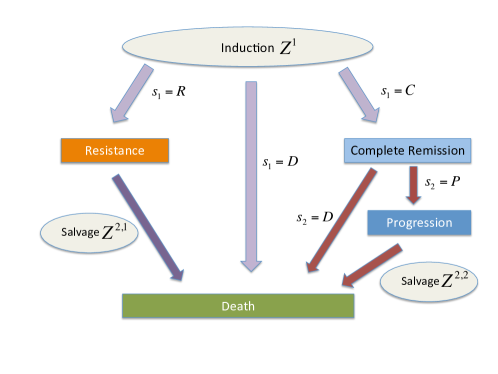
Figure 1: The scheme

Since all elements of a DTR may affect $T$, the clinically relevant problem is optimizing the entire regime, rather than the treatment at one particular stage. Most clinical trials or data analyses attempt to reduce variability by focusing on one stage of the actual DTR, usually frontline or first salvage treatment, or by combining stages in some manner. This often misrepresents actual clinical practice, and consequently conclusions may be very misleading. For example, an aggressive frontline cancer chemotherapy may maximize the probability of $C$, but it may cause so much immunologic damage that any salvage treatment given after rapid relapse, i.e. short $T^{C,P}$, may be unlikely to achieve a second remission. In contrast, a milder induction treatment may be suboptimal to eradicate the tumor, but it may debulk the tumor sufficiently to facilitate surgical resection. Such synergies may have profound implications for clinical practice, especially because effects of multi-stage treatment regimes often are not obvious and may seem counter-intuitive. Physicians who have not been provided with an evaluation of the composite effects of entire regimes on the final outcome may unknowingly set patients on pathways that include only inferior regimes.

A major practical advantage of BNP models is that they often provide better fits to complicated data structures than can be obtained using parametric model-based methods. In our motivating application, where leukemia patients were randomized among initial chemotherapy treatments but not among later salvage therapies, the BNP model provides good fits for each transition time distribution conditional on previous history. Failure to randomize patients in treatment stages after the first is typical in clinical trials, most of which ignore all but the first stage of therapy. In contrast, sequential multi-arm randomized treatment (SMART) designs, wherein patients are re-randomized at stages after the first, have been used in oncology trials (Thall et al.,, 2000; Thall et al., 2007a, ; Thall et al., 2007b, ), and are being used increasingly in trials to study multi-stage adaptive regimes for behavioral or psychological disorders (Dawson and Lavori,, 2004; Murphy et al., 2007a, ; Murphy et al., 2007b, ; Connolly and Bernstein,, 2007).

While re-randomization is desirable, it is not commonly done and inference has to adjust for this lack of randomization. A wide array of methods have been proposed for evaluating DTRs from observational data and longitudinal studies, beginning with the seminal papers by Robins, (1986, 1987, 1989, 1997) on G-estimation of structural nested models. Additional references include applications to longitudinal data in AIDS (Hernán et al.,, 2000), inverse probability of treatment weighted (IPTW) estimation of marginal structural models (Murphy et al.,, 2001; van der Laan and Petersen,, 2007; Robins et al.,, 2008), G-estimation for optimal DTRs (Murphy,, 2003; Robins,, 2004), and a review by Moodie et al., (2007). A variety of methods have been developed to evaluate DTRs from clinical trials (Lavori and Dawson,, 2000; Thall et al.,, 2002; Murphy,, 2005). For survival analysis, Lunceford et al., (2002) introduced ad hoc estimators for the survival distribution and mean restricted survival time under different treatment policies. These estimators, although consistent, were inefficient and did not exploit information from auxiliary covariates. Wahed and Tsiatis, (2006) derived more efficient, easy-to-compute estimators that included auxiliary covariates for the survival distribution and related quantities of DTRs. Their estimators compared DTRs using data from a two-stage randomized trial, in which two options were available for both stages and the second-stage treatment assignments were determined by randomization. However, these estimators must be adapted for more general or more complicated designs that permit various numbers of treatment options at each stage and involve the scenarios where second-stage treatment is not randomized, but rather determined by the attending physicians.

In settings where the DTR’s final overall time, such as survival time, is the sum of a sequence of transition times, we propose a Bayesian nonparametric approach that employs a nonparametric regression model for (the logarithm of) each transition time conditional on the most recent history of actions and outcomes. We assume a dependent Dirichlet process prior with Gaussian process base measure (DDP-GP), and compute a joint posterior by Markov chain Monte Carlo (MCMC) sampling. To address the important issue that Bayesian analyses depend on prior assumptions, we provide guidelines for using empirical Bayes methods to establish prior hyperparameters. Posterior analyses include estimation of posterior mean overall outcome times and credible intervals for each DTR.

The rest of the paper is organized as follows. In Section 2 we review the motivating study, and give a brief review of DTRs in settings with successive transition times in Section 3. We present the DDP-GP model in Section 4. A simulation study of the BNP approach in single-stage and multi-stage regimes, with comparison to frequentist IPTW, is summarized in Section 5. We re-analyze the leukemia trial data in Section 6, and close with brief discussion in Section 7.

2 Motivating Study

Our proposed methodology is motivated by a clinical trial conducted at The University of Texas M.D. Anderson Cancer Center to evaluate chemotherapies for acute myelogenous leukemia (AML) or myelo-dysplastic syndrome (MDS). Patients were randomized fairly among four front-line combination chemotherapies for remission induction: fludarabine + cytosine arabinoside (ara-C) plus idarubicin (FAI), FAI + all-trans-retinoic acid (ATRA), FAI + granulocyte colony stimulating factor (GCSF), and FAI + ATRA + GCSF. The goal of induction therapy for AML/MDS is to achieve complete remission ($C$), a necessary but not sufficient condition for long-term survival. Patients who do not achieve $C$, or who achieve $C$ but later relapse, are given salvage treatments as another attempt to achieve $C$. Following conventional clinical practice, patients were not randomized among salvage therapies, which were chosen by the attending physicians based on clinical judgment. Since there were many types of salvage, these are broadly classified into two categories as either containing high dose ara-C (HDAC) or not. This data set was analyzed initially using conventional methods (Estey et al.,, 1999), including logistic regression, Kaplan-Meier estimates, and Cox model regression, including comparisons of the induction therapies in terms of OS that ignored possible effects of salvage therapies.

Figure 1 illustrates the actual possible therapeutic pathways and outcomes of the patients during the trial, which is typical of chemotherapy for AML/MDS. Death might occur (1) during induction therapy, (2) following salvage therapy if the disease was resistant to induction, (3) during $C$, or (4) following disease progression after $C$. Wahed and Thall, (2013) re-analyzed the data from this trial by accounting for the structure in Figure 1, and identified 16 DTRs including both frontline and salvage therapies. To correct for bias due to the lack of randomization in estimating the mean OS times, they used both IPTW (Robins and Rotnitzky,, 1992) and G-estimation based on a frequentist likelihood. In the G-estimation, for each transition time they first fit accelerated failure time (AFT) regression models using Weibull, exponential, log-logistic or log-normal distributions, and chose the distribution having smallest Bayes information criterion (BIC). They then performed likelihood-based G-estimation by first fitting each conditional transition time distribution regressed on patient baseline covariates and previous transition times, and then averaging over the empirical covariate distribution.

Like Wahed and Thall, the primary goal of our analyses of the AML/MDS dataset is to estimate mean OS and determine the optimal regime. We build on their approach by replacing the parametric AFT models for transition times with the DDP-GP model. We also demonstrate the usefulness of the BNP regression model for G-estimation in simulation studies of single-stage and multi-stage regimes in which treatment assignments depend on patient covariates.

3 Dynamic Regimes with Stochastic Transition Times

Denote the set of possible disease states by $\{0,1,\cdots,n_{\mbox{state}}\},$ with $0$ denoting the patient’s initial state before receiving the first treatment. The pairs of states $(s_{\ell-1},s_{\ell})$ for which a transition $s_{\ell-1}\rightarrow s_{\ell}$ is possible at stage $\ell$ of the patient’s therapy depend on the particular regime. Here $s_{0}$ refers to the patient’s initial state, before start of therapy. We will identify specific states using letters such as $P$, $C$, etc., as in the earlier examples, to replace the generic integers. For example, in cancer therapy, $s_{\ell-1}\rightarrow C$ means that a patient’s disease has responded to treatment, $P\rightarrow D$ means a patient with progressive disease has died, and of course $D\rightarrow s_{\ell}$ is impossible. We denote the transition time from state $s_{\ell-1}$ to state $s_{\ell}$ in stage $\ell$ of treatment by $T^{\ell,(s_{\ell-1},s_{\ell})}$, for ${\ell}=1,\cdots,n_{\mbox{stage}},$ the maximum number of stages in the DTR. When no ambiguity arises we simply write $T^{r,s}$ for the transition time from state $r$ to $s$. To simplify notation for the transition time distributions, we denote the history of all covariates, treatments, and previous transition times through $\ell$ stages, before observation of $T^{\ell,(s_{\ell-1},s_{\ell})}$ but including the stage $\ell$ action $Z^{\ell}$ by ${\bm{x}}^{\ell}$ = $({\cal H}^{\ell-1},Z^{\ell})$ = $({\bm{x}}^{0},Z^{1},T^{1,(s_{0},s_{1})},\cdots,Z^{\ell})$, with ${\bm{x}}^{0}$ = $\mathcal{H}^{0}$. Thus, a DTR is ${\boldsymbol{Z}}$ = $(Z^{1},Z^{2},\ldots)$, a sequence of actions for all possible stages. When no meaning is lost, we will write $T^{\ell,(s_{\ell-1},s_{\ell})}$ as $T^{k},$ where $k=1,\ldots,n_{T}$ is a running index of all possible state transitions. For example, in Figure 1 we have up to $n_{\mbox{stage}}=3$ stages and $n_{T}=7$ possible transitions. Similarly, we will write $\bm{x}^{k}$ for the corresponding covariate vector. Our use of a single index to identify stage is a slight abuse of notation since, for example, the actual second stage of therapy might differ depending on the sequence of outcomes. For example, stage 2 treatment $Z^{2}$ of a patient with sequence $({\bm{x}}^{0},Z^{1},T^{1,(0,R)},Z^{2})$ is first salvage for resistant disease during induction with $Z^{1}$, while stage 3 treatment $Z^{3}$ of a patient with sequence $({\bm{x}}^{0},Z^{1},T^{1,(0,C)},T^{2,(C,P)},Z^{3})$ is first salvage for progressive disease after achieving response initially with $Z^{1}.$ This latter example could be elaborated if, under a different regime, consolidation therapy, $Z^{2}$, were given for patients who enter $C$, in which case the sequence would be $({\bm{x}}^{0},Z^{1},T^{1,(0,C)},Z^{2},T^{2,(C,P)},Z^{3}).$

Below we will develop a general BNP model for all possible conditional distributions of the form $p(T^{k}~{}|~{}{\bm{x}}^{k})$ = $p(T^{\ell,(s_{\ell-1},s_{\ell})}~{}|~{}{\bm{x}}^{\ell}).$ This determines the likelihood for all possible sequences of treatments and transition times through $n_{T}$ transitions as the product

$${\cal L}\ =\ \prod_{k=1}^{n_{T}}\,p(T^{k}~{}|~{}{\bm{x}}^{k}).$$ (1)

The overall time for any counterfactual sequence of transition times is the sum $T\ =\ \sum_{k=1}^{n_{T}}\,T^{k}$. Our goal is to estimate the mean of $T$ for each possible ${\boldsymbol{Z}}.$

4 A Nonparametric Bayesian Model for DTR’s

4.1 DDP and Gaussian Process Prior

To specify the BNP model, we denote $Y^{k}$ = log$(T^{k})$ and write the distribution of $[Y^{k}~{}|~{}{\bm{x}}^{k}]$ as $F^{k}(\cdot~{}|~{}{\bm{x}}^{k})$. For convenience, we will refer to ${\bm{x}}^{k}$ as ‘covariates’. We construct a BNP survival regression model for each $F^{k}(\cdot~{}|~{}{\bm{x}}^{k})$ by successive elaborations, starting with a model for a discrete random distribution $G(\cdot)$. We then use a Gaussian kernel to extend this to a prior for a continuous random distribution $F(\cdot)$, and finally endow the kernel means with a regression structure by expressing them as functions of ${\bm{x}}^{k}.$ The latter construction extends $F$ to a family $\{F(\cdot\mid\bm{x}^{k})\}$, indexed by $\bm{x}^{k}$. The construction of $G(\cdot)$ and $F(\cdot)$ is briefly outlined below, by way of a brief review of BNP models. In the end we will only use the last model $\{F(\cdot\mid\bm{x}^{k})\}$, which we use as sampling model for $Y^{k}$. See, for example, Müller and Mitra, (2013) and Müller and Rodriguez, (2013) for more extensive reviews of BNP inference.

The Dirichlet process (DP) prior first was proposed by Ferguson, (1973) as a probability distribution on a measurable space of probability measures. The DP is indexed by two hyperparameters, a base measure, $G_{0},$ and a precision parameter, $\alpha>0$. If a random distribution $G$ follows a DP prior, we denote this by $G\sim DP(\alpha,G_{0})$. Denoting a beta distribution by $\mbox{Be}(a,b)$, if $G\sim DP(\alpha,G_{0})$ then $G(A)\sim\mbox{Be}\{\alpha G_{0}(A),\alpha[1-G_{0}(A)]\}$ for any measurable set $A$, and in particular $E\{G(A)\}=G_{0}(A).$ Let $\delta(\theta)$ denote a point mass at $\theta$. Sethuraman, (1991) provided a useful representation of the DP as $G=\sum_{h=0}^{\infty}w_{h}\delta(\theta_{h})$, where $\theta_{h}\mathrel{\mathop{\sim}\limits^{\mbox{\footnotesize i.i.d.}}}G_{0}$, and the weights $w_{h}$ are generated sequentially from rescaled Beta distributions as $w_{h}/(1-\sum_{r=1}^{h-1}w_{r})\sim Be(1,\alpha)$, the so-called “stick-breaking” construction. The discrete nature of $G$ is awkward in many applications. A DP mixture model extends the DP model by replacing each point mass $\delta(\theta_{h})$ with a continuous kernel centered at $\theta_{h}$. Without loss of generality, we will use a normal kernel. Let $N(\cdot;\;\mu,\sigma)$ denote the measure of a normal distribution with mean $\mu$ and standard deviation (sd) $\sigma$. The DP mixture model assumes

$$G=\sum_{h=0}^{\infty}\ w_{h}N(\cdot\;;\theta_{h},\sigma).$$ (2)

The use and interpretation of (2) is very similar to that of a finite mixture of normal models. In practical applications, the sum in (2) is often truncated at a reasonable finite value. This model is useful for density estimation under i.i.d. sampling from an unknown distribution, and it provides good fits to a wide variety of datasets because a mixture of normals can closely approximate virtually any distribution (Ishwaran and James,, 2001).

To include the regression on covariates that we will need for the survival model of each conditional transition time distribution, $(Y^{k}~{}|~{}{\bm{x}}^{k})$, we extend the DP mixture to a dependent DP (DDP), which was first proposed by MacEachern, (1999). The basic idea of a DDP is to endow each $\theta_{h}^{k}$ with additional structure that specifies how it varies as a function of covariates ${\bm{x}}^{k}.$ Writing this regression function as $\theta^{k}_{h}({\bm{x}}^{k})$ for each summand in $(\ref{eq:dpm})$, and returning to the conditional transition time distributions, we assume that

$$F^{k}(y~{}|~{}{\bm{x}}^{k})=\sum_{h=0}^{\infty}w^{k}_{h}\,N(y;\ \theta_{h}^{k}({\bm{x}}^{k}),\,\sigma^{k}).$$ (3)

This form of the DDP, which includes both the convolution with a normal kernel and functional dependence on covariates, provides a very flexible regression model.

To complete our specification of the DDP, we will assume that the $\theta^{k}_{h}(\cdot)$’s are independent realizations from a Gaussian process prior. The Gaussian process first was popularized by O’Hagan and Kingman, (1978) in Bayesian inference for a random function (unrelated to the use in a DDP prior). For more recent discussions see, for example, Rasmussen and Williams, (2006); Neal, (1995); Shi et al., (2007). Temporarily suppressing the transition index $k$ and running index $h$ in $(\ref{eq:Fx})$, and denoting ${\bm{x}}$ = $(x_{1},\cdots,x_{n})$, a Gaussian process is a stochastic process $\theta(\cdot)$ in which $\theta({\bm{x}})$ = $\{\theta(x_{1}),\ldots,\theta(x_{n})\}^{\prime}$ has a multivariate normal distribution with mean vector $\mu({\bm{x}})=(\mu(x_{1}),\ldots,\mu(x_{n}))$ and $(n\times n)$ covariance matrix $C({\bm{x}})$ for $\bm{x}$ of any dimension $n\geq 1$. We denote this by $\theta\sim GP(\mu,C).$

We use the GP prior to define the dependence of $\theta_{h}^{k}(\bm{x}^{k})$ as a function of $\bm{x}^{k}$ by assuming $\{\theta_{h}^{k}(\bm{x}_{k})\}\sim\ GP(\mu_{h}^{k},C^{k})$, as a function of $\bm{x}_{k}$, for fixed $h$. We will refer to the DDP with a convolution using a normal kernel and a Gaussian process prior on the normal kernel means as a DDP-GP model. While the mean and covariance processes of the GP can be quite general, in practice, $C^{k}({\bm{x}}^{k})$ often is parameterized as a function $C^{k}_{ij}=C(x^{k}_{i},x^{k}_{j};\xi^{k})$, where $\xi^{k}$ is a vector of hyperparameters, and the mean function is indexed similarly by hyperparameters $\bm{\beta}_{h}^{k}$ and written as $\mu_{h}^{k}(\bm{x}^{k}\mid\bm{\beta}_{h}^{k})$. In the DTR setting, since each covariate vector ${\bm{x}}^{k}$ is a history, its entries can include baseline covariates, transition times, and indicators of previous treatments or actions. To obtain numerically reasonable parameterizations of the Gaussian process functions $C^{k}$ and $\mu_{h}^{k}$, we standardize numerical-valued covariates such as age. We now have

$$\{\theta^{k}_{h}(\bm{x}^{k})\}\sim\ GP(\mu_{h}^{k}(\bm{x}^{k}),C^{k}(\bm{x}^{k})),\ \ \ \ \ \ h=1,2,...$$

To specify the form of $\mu_{h}^{k}$ and $C^{k},$ let $i=1,2,\cdots,$ index patients, so that $\bm{x}^{k}_{i}$ is the history of patient $i$ at transition $k$, and define the indicator $\delta_{ij}=I(i=j)$ = 1 if $i=j$ and 0 otherwise. We model the mean function $\mu_{h}^{k}(\cdot)$ as a linear regression, by assuming that

$$\mu_{h}^{k}(\bm{x}^{k}_{i})=\bm{x}^{k}_{i}\bm{\beta}_{h}^{k}.$$ (4)

For patients $i$ and $j$, we assume that the covariance process takes the form

$$C^{k}(\bm{x}^{k}_{i},\bm{x}^{k}_{j})=\exp\{-\sum_{m=1}^{M^{k}}(x^{k}_{im}-x^{k}_{jm})^{2}\}+\delta_{ij}J^{2},\ \ \ i,j=1,\dots,n,$$ (5)

where $M^{k}$ is the number of covariates at transition $k$ and $J$ is the variance on the diagonal reflecting the amount of jitter (Bernardo et al.,, 1999), which usually takes a small value (e.g, $J=0.1$). For binary covariates, the quadratic form in (5) reduces to counting the number of binary covariates in which two patients differ. If desired, additional hyperparameters could be introduced in (5) to obtain more flexible covariance functions. However, in practice this form of the covariance matrix yields a strong correlation for observations on patients with very similar $\bm{x}^{k}$, and has been adopted widely (Williams,, 1998).

Combining all of these structures, we denote the model for conditional distribution of the $k^{th}$ transition time as

$$F^{k}\sim\mbox{DDP-GP}\left\{\{\mu_{h}^{k}\},C^{k};\alpha^{k},\,\{\bm{\beta}_{h}^{k}\},\,\sigma^{k}\right\},$$ (6)

recalling that the weights of the DDP are generated sequentially as $w^{k}_{h}/(1-\sum_{r=1}^{h-1}w^{k}_{r})\sim Be(1,\alpha^{k})$. For later reference we state the full model,

$$p(y_{i}^{k}\mid\bm{x}_{i}^{k},F^{k})=F^{k}(y_{i}^{k}\mid\bm{x}_{i}^{k})$$

$$F^{k}\sim\mbox{DDP-GP}\left\{\{\mu_{h}^{k}\},C^{k};\alpha^{k},\,\{\bm{\beta}_{h}^{k}\},\,\sigma^{k}\right\}$$ (7)

$k=1,\ldots,n_{T}$.

4.2 Determining Prior Hyperparameters

As priors for $\bm{\beta}_{h}^{k}$ in (4) we assume $\bm{\beta}_{h}^{k}\sim\ N(\bm{\beta}_{0}^{k},\Sigma_{0}^{k})$ for each transition $k$, $h=1,2,\dots$. For the normal pdfs of the DDP mixture models we assume the precision parameters follow the same prior $(\sigma^{k})^{-2}\mathrel{\mathop{\sim}\limits^{\mbox{\footnotesize i.i.d.}}}\ \mbox{Ga}(\lambda_{1},\lambda_{2})$ and, similarly, for the parameters that determine the weights of the DDP mixture under the stick-breaking construction we assume $\alpha^{k}\mathrel{\mathop{\sim}\limits^{\mbox{\footnotesize i.i.d.}}}\ \mbox{Ga}(\lambda_{3},\lambda_{4}).$

To apply the DDP-GP model, one must first determine numerical values for the fixed hyperparameters $\{\bm{\beta}_{0}^{k},$ $\Sigma_{0}^{k},k=1,2,...\}$ and ${\bm{\lambda}}$ = $(\lambda_{1},\lambda_{2},\lambda_{3},\lambda_{4}).$ This is a critical step. These numerical hyperparameter values must facilitate posterior computation, and they should not introduce inappropriate information into the prior that would invalidate posterior inferences. With this in mind, the hyperparameters $(\bm{\beta}_{0}^{k},\Sigma_{0}^{k})$ for the $k^{th}$ transition time covariate effect distribution may be obtained via empirical Bayes by doing a preliminary fits of a lognormal distribution $Y^{k}$ = log$(T^{k})\sim$ $N(\bm{x}^{k}\bm{\beta}^{k}_{0},\sigma^{k}_{0})$ for each transition $k.$ The covariate effect estimates then can be used as the values of $\bm{\beta}^{k}_{0}$. Similarly, we assume a diagonal matrix for $\Sigma_{0}^{k}$ with the diagonal values also obtained from the preliminary fit of the lognormal distribution. Once an empirical estimate of $\sigma^{k}$ is obtained, one can tune $(\lambda_{1},\lambda_{2})$ so that the prior mean of $\sigma^{k}$ equals the empirical estimate and the variance equals 1 or a suitably large value to ensure a vague prior. In contrast, information about $\alpha^{k}$ typically is not available in practice, and an empirical Bayes approach cannot be applied to determine $(\lambda_{3},\lambda_{4})$. However, setting $\lambda_{3}=\lambda_{4}$ = 1 gives a Gamma(1, 1) distribution, which has mean 1 and variance 1, and is a well behaved, noninformative prior for $\alpha^{k}$ that may be used generally when fitting the DDP-GP model.

This approach works in practice because the parameter $\bm{\beta}_{0}^{k}$ specifies the prior mean for the mean function of the GP prior, which in turn formalizes the regression of $T^{k}$ on the covariates $\bm{x}^{k}$, including treatment selection. The imputed treatment effects hinge on the predictive distribution under that regression. Excessive prior shrinkage could smooth away the treatment effect that is the main focus. The use of an empirical Bayes type prior in the present setting is similar to empirical Bayes priors in hierarchical models. This type of empirical Bayes approach for hyperparameter selection is commonly used when a full prior elicitation is either not possible or is impractical. Inference is not sensitive to values of the hyperparameters $\bm{\lambda}$ that determine the priors of $\sigma^{k}$ and $\alpha^{k}$ for two reasons. First, the standard deviation $\sigma^{k}$ is the scale of the kernel that is used to smooth the discrete random probability measure generated by the DDP prior. It is important for reporting a smooth fit, that is for display, but it is not critical for the imputed fits in our regression setting. Assuming some regularity of the posterior mean function, smoothing adds only minor corrections. Second, the total mass parameter $\alpha^{k}$ determines the number of unique clusters formed in the underlying Polya urn. Because most clusters are small a priori, including many singleton clusters, varying the number of these clusters by changing the prior of $\alpha^{k}$ does not significantly change the posterior predictive values that are the basis for the proposed inference.

The conjugacy of the implied multivariate normal on $\{\theta_{h}^{k}(\bm{x}^{k}),h=0,1,\dots\}$ and the normal kernel in (3) greatly simplify the computations, since any Markov chain Monte Carlo (MCMC) scheme for DP mixture models can be used. MacEachern and Müller, (1998) and Neal, (2000) described specific algorithms to implement posterior MCMC simulation in DPM models. Ishwaran and James, (2001) developed alternative computational algorithms based on finite DPs, which truncated (2) after a finite number of terms. We provide details of MCMC computations in the online supplement.

5 Simulation Studies

We conducted three simulation studies to evaluate the performance of the proposed DDP-GP model as a tool for estimating the mean of $T$ in survival regression settings. The studies focused, respectively, on estimation of (i) survival regression; (ii) regime effects in a study with two treatment arms and single-stage regimes; and (iii) regime effects in a study with eight multi-stage regimes. For each of the latter two studies, the treatment assignment probabilities depend on patient covariates. That is, we introduce a treatment selection bias. In all three simulations, we implement inference under DDP-GP models. In (i) we use a single survival regression $F(Y_{i}\mid\bm{x}_{i})$ for a patient-specific baseline covariate vector $\bm{x}_{i}$. For (ii) we still use a single DDP-GP model $F(Y_{i}\mid\bm{x}_{i},Z_{i})$, now adding a treatment indicator $Z_{i}$ to the survival regression. In (iii) we use independent DDP-GP models $F^{k}(Y_{i}^{k}\mid\bm{x}_{i}^{k})$ for multiple transition times, $k=1,\ldots,n_{T}$, similar to the motivating application. For all three simulation studies, the hyperprior parameters were determined using the empirical Bayes approach described earlier. For all posterior computations, the MCMC algorithm was implemented with an initial burn-in of 2,000 iterations and a total of 5,000 iterations, thinning out in batches of 10. This worked well in all cases, with convergence diagnostics using the R package coda showing no evidence of practical convergence problems. Traceplots and empirical autocorrelation plots (not shown) for the imputed parameters indicated a well mixing Markov chain.

5.1 Survival Time Regression

The first simulation was designed to study the DDP-GP regression model by comparing inference for a survival function with the simulation truth. In this study, we did not evaluate a regime effect, but rather focused on inference for the survival curve.

For each subject, we generated $T$ = survival time, the covariates $x_{1}$ = tumor size (0=small, 1=large) and $x_{2}$ = body weight, and $x_{3}$ = a biomarker (0=absent, 1=present). We assumed that small and large tumor sizes each had probability .50. Body weights were computed by sampling from a uniform distribution, $\mathrm{Unif}(80,150)$, with the covariate $x_{2}$ defined by shifting and scaling to obtain mean 0 and variance 1. The biomarker was associated with tumor size, as follows. Patients in the large tumor size group were biomarker negative with probability 0.7 and biomarker positive with probability 0.3. Patients with small tumor size were biomarker negative with probability 0.3 and biomarker positive with probability 0.7. Let $Y\sim\mbox{LN}(m,s)$ denote a log normal random variable $Y=\log T$ for $T\sim\mbox{N}(m,s)$. By a slight abuse of notation, we also use $\mbox{LN}(m,s)$ to denote the log normal p.d.f. Let $\bm{x}_{i}=(1,\mathrm{x}_{i,1},\mathrm{x}_{i,2},\mathrm{x}_{i,3})$ denote the covariates for patient $i$. We simulated each sample $Y_{1},\cdots,Y_{n}$ of $n$ observations from a mixture of lognormal distributions, $Y_{i}|\bm{x}_{i}\ \sim\ 0.4\ \mbox{LN}(\bm{x}_{i}\bm{\beta}_{1},\sigma^{2})+0.6\ \mbox{LN}(\bm{x}_{i}\bm{\beta}_{2},\sigma^{2})$, where the true covariate parameters of the mixture components were $\bm{\beta}_{1}=(1,2,-2,1)^{\prime}$ and $\bm{\beta}_{2}=(2,-1,3,-3)^{\prime}$, with $\sigma^{2}=0.4$. For comparison, we also fit an AFT regression model, assuming

$$Y_{i}\ =\ \log(T_{i})=\bm{x}_{i}^{\prime}\bm{\beta}+\sigma\epsilon_{i},\ \ \ i=1,\dots,n$$

with $\epsilon_{i}$ following an extreme value distribution, so that $T_{i}$ follows a Weibull distribution.

In this simulation, we considered four scenarios, with $n=50,100,$ or $200$ observations without censoring or $n=200$ with 23% censoring. For each scenario, $N=1,000$ trials were simulated. For each simulated data set we fit a DDP-GP survival regression model $F(Y_{i}\mid\bm{x}_{i})$. For simulation $j$, let $\overline{S}(t\mid\bm{x})=p(T_{n+1}\geq t\mid\bm{x}_{n+1,j}=\bm{x},data)$ denote the posterior expected survival function for a future patient with covariate $\bm{x}$. Using the empirical distribution $\frac{1}{n}\sum_{i=1}^{n}\delta_{\bm{x}_{ij}}$ to marginalize w.r.t. $\bm{x}_{n+1,j}$ and averaging across simulations, we get

$$\overline{S}(t)=\frac{1}{N}\,\sum_{j=1}^{N}\,\frac{1}{n}\sum_{i=1}^{n}\overline{S}(t\mid\bm{x}_{ij}).$$

Figure 2 compares $\overline{S}(\cdot)$ under the DDP-GP model with the simulation truth

$$S_{0}(t)=\frac{1}{N}\,\sum_{j=1}^{N}\,\frac{1}{n}\,\sum_{i=1}^{n}S_{0}(t\mid\bm{x}_{ij}),$$

and a maximum likelihood estimate (MLE) under a Weibull AFT model. In each scenario, the true curve is given as a solid black solid line, the MLE of the survival functions under the AFT regression model assuming a Weibull distribution as a solid green solid line, and the posterior mean survival function under the DDP-GP model as a solid red line with point-wise 90% credible bands as two dotted red lines.

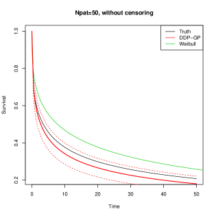
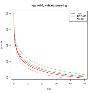
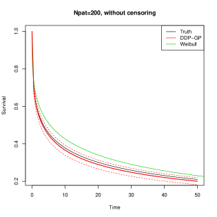
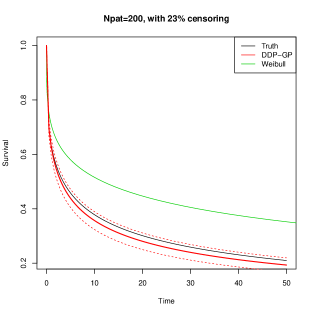
Figure 2: Simulation example 1. True mean survival functions (black color) and estimated mean survival functions under the DDP-GP model (red color) for sample sizes $n=50,100,200$ and $n=200$ with 23% censoring for 1,000 simulations. For comparisons, we also show the MLE under an AFT regression with Weibull distribution (green color). In all cases, the point-wise 90% credible bands are also displayed as the region between two dotted red lines.

In all four scenarios, the DDP-GP model based estimate reliably recovered the shape of the true survival function and avoided the excessive bias seen with the Weibull MLE. As expected, the three scenarios without censoring show that increasing sample size gives more accurate estimation. With 23% censoring, the DDP-GP estimate becomes less accurate, but it still is much closer to the simulation truth than the Weibull MLE.

5.2 Estimating a Treatment Effect in Single-stage Regimes

The second simulation study was designed to investigate inference under the DDP-GP model for a regime effect in a single-stage treatment setting. The simulated data represent what might be obtained in an observational setting where treatment is chosen by the attending physician based on patient covariates, rather than from a fairly randomized clinical trial. We simulated a binary treatment indicator $Z_{i}\in$ {0=control, 1=experimental} that depended on two continuous covariates, $\bm{x}_{i}=(L_{i},W_{i})$, for $n=100$ patients, $i=1,\dots,n$. For example, $L_{i}$ could be a patient’s creatinine to quantify kidney function, and $W_{i}$ could be body weight. We generated $L_{i}$ from a mixture of normals, $L_{i}\sim\frac{1}{2}N(40,10^{2})+\frac{1}{2}N(20,10^{2})$, which could correspond to a subgroup of patients having worse kidney function (higher creatinine level) due to damage from prior chemotherapy. We assumed that $W_{i}\sim\mbox{Unif}(-\sqrt{12},\sqrt{12})$, a uniform with zero mean and unit standard deviation, as could arise from standardizing a uniformly distributed raw variable. We generated the treatment indicators using the modified logistic regression model

$$p(Z_{i}=1\mid L_{i},W_{i})=\left\{\begin{array}[]{l l}0.05&\quad\text{if $\left\{1+\exp[-2(L_{i}-30)/10]\right\}^{-1}\leq 0.05$ }\\ 0.95&\quad\text{if $\left\{1+\exp[-2(L_{i}-30)/10]\right\}^{-1}\geq 0.95$}\\ \left\{1+\exp[-2(L_{i}-30)/10]\right\}^{-1}&\quad\text{otherwise},\end{array}\right.$$

that is, a logistic regression with intercept 30 and slope 1/5 truncated at 0.05 and 0.95. This produces a very unbalanced treatment assignment, for example, $p(Z_{i}=1\mid L_{i}=40)=0.88$ versus $p(Z_{i}=1\mid L_{i}=20)=0.12$. This could arise in a setting where standard therapy, $Z=0$, is known to be nephrotoxic, while it is believed by most of the treating physicians that the experimental therapy, $Z_{i}=1$, is not, so patients with high creatinine are more likely to be given the experimental therapy. In this simulation study, the goal is to estimate the comparative effect on survival of the experimental therapy versus the control. In the two treatment arms, we generated patients’ responses from

$$Y(1)\sim\frac{1}{2}\ \mathrm{N}(3-0.2L+\sqrt{L}-0.1W,\ \sigma)+\frac{1}{2}\ \mathrm{N}(2-0.2L+\sqrt{L}-0.1W,\ \sigma)$$

and

$$Y(0)\sim\mathrm{N}(-0.2L+\sqrt{L}-0.1W,\ \sigma),$$

with $\sigma=0.4$. We simulated 1,000 trials. Note that under the simulation truth the treatment effect, $E[Y(1)-Y(0)\mid\bm{x}=(L,W)]=2.5$, is constant across $L,W$.

Figure 3(a) plots the simulation truth for the mean response curve under $Z=1$ and $Z=0$ versus $L$, with $W\equiv 0$, in one randomly selected trial. The upper red solid curve represents $E[Y(1)\mid L,W=0]$ and the lower black curve represents $E[Y(0)\mid L,W=0]$. The red dots close to the upper curve are the observations for experimental arm patients and the black dots close to the lower curve are the observations for the control arm patients. We define an average treatment effect for the entire population under the simulation truth as $\frac{1}{n}\sum_{i=1}^{n}E[Y_{i}(1)-Y_{i}(0)]=2.5$.

We implemented inference for a survival regression $F(Y_{i}\mid\bm{x}_{i},Z_{i})$ using the proposed DDP-GP model. Figure 3(b) summarizes inference for the data from panel (a). Let $\hat{Y}_{i}(z)=E(Y_{n+1}\mid L_{n+1}=L_{i},W_{n+1}=W_{i},Z_{i}=z,data)$ denote the posterior expected response for a future patient $n+1$. We define an estimated average treatment effect as $\frac{1}{n}\sum_{i=1}^{n}[\hat{Y}_{i}(1)-\hat{Y}_{i}(0)]$. Figure 3(b) shows the estimated average treatment effect (horizontal red line), and credible intervals for individual effects $\hat{Y}_{i}(1)-\hat{Y}_{i}(0)$ (vertical line segments, located at $L_{i}$).

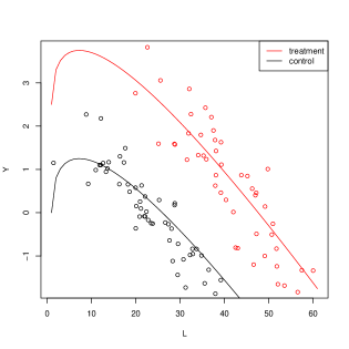
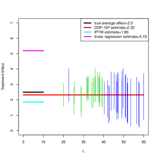
(a)	(b)

Figure 3: Simulation example 2. (a) Simulated data for one (treatment, control) pair. The upper red solid curve represents $E[Y(1)\mid X]$, the lower black curve represents $E[Y(0)\mid X]$ given $W=0$. The red dots close to the upper curve are the treated observations and the black dots close to the lower curve are the untreated. (b) Average treatment effect estimations. The black solid line represents the true average treatment effect, the red line represents posterior mean treatment effect estimates under the DDP-GP model, turquoise blue represents IPTW estimate, the heliotrope line represents the linear regression estimate. The vertical line segments are marginal 90% posterior intervals for the treatment effect at each $L$ value from treated observations.

For comparison, we also applied both linear regression (LR) and an IPTW method to the simulated data to estimate the average treatment effect. The LR method fits observations from both treatments using linear predictor functions and estimates the average treatment effect, assuming $Y_{i}(1)=\beta_{10}+\beta_{11}L_{i}+\beta_{12}W_{i}+\epsilon_{1i}$ and $Y_{i}(0)=\beta_{00}+\beta_{01}L_{i}+\beta_{02}W_{i}+\epsilon_{0i}$. Denoting the least squares estimates by $\hat{\beta}_{zj}$ for $z=0,1$ and $j=0,1,2,$ the estimated means are $\hat{E}\{Y_{i}(z)\}=\hat{\beta}_{z0}+\hat{\beta}_{z1}L_{i}+\hat{\beta}_{z2}W_{i}$. We define an estimated average treatment effect as $\frac{1}{n}\sum_{i}\,[\hat{E}\{Y_{i}(1)\}-\hat{E}\{Y_{i}(0)\}]$. The IPTW method assigns each patient $i$ a weight $b_{i}$ equal to the inverse of an estimate of $p(Z_{i}\mid\bm{x}_{i})$, the conditional probability of receiving his or her actual treatment (Robins et al.,, 2000), with the estimate obtained by fitting a logistic regression model. The effect of weighting is to create a pseudo-population consisting of $b_{i}$ copies of each patient $i$. For example, if $b_{i}=5$ then five copies of the $i^{th}$ patient are contributed to the pseudo-population. Thus, for $z$ = 0 or 1, we define an estimated mean outcome

$$\mathrm{IPTW}(Z=z)=\frac{\sum_{i}I(Z_{i}=z)b_{i}Y_{i}}{\sum_{i}I(Z_{i}=z)b_{i}},$$

and a corresponding average treatment effect estimate $\mathrm{IPTW}(Z=1)-\mathrm{IPTW}(Z=0).$ The DDP-GP point estimate of the average effect of the treatment is the posterior mean 2.31 with 90% posterior credible interval (1.89, 2.96). The LR fit yields an overestimate, 4.13, while IPTW yields an underestimate, 1.11. In Figure 3(b), the red horizontal line represents the posterior mean treatment effect estimate obtained from the DDP-GP model. The short horizontal black, turquoise blue and heliotrope solid lines represent the true average treatment effect, IPTW estimate, and LR estimate, respectively. The vertical green and blue segments are marginal 90% posterior credible intervals for the treatment effect at each $L$ value from treated observations. Lengths of posterior credible intervals larger than 2 are highlighted by blue segments. Note that the uncertainty bounds grow wider in the range where there is less overlap across treatment groups, that is, over a range of covariate values for which we do not observe reliable empirical counterfactuals for each data point (e.g. $L>50$). Most of the credible intervals reasonably cover the true treatment effect.

Figure 3 reports inference for one hypothetical data set. For a more meaningful comparison we carried out extensive simulation and report the distribution of estimated regime effects across repeat simulations. We compared the regime effects estimates obtained by DDP-GP, IPTW, and LR based on data from 1,000 simulated trials. Figure 4 gives density plots of the estimated regime effects. Compared to the estimates obtained from DDP-GP, the IPTW estimates are much more variable, ranging from 1.14 to 7.13. In general, the LR estimates are highly biased, and overestimate the true effects. The distribution of estimated regime effects under the DDP-GP model is remarkably narrowly centered around the simulation truth, in comparison with the two alternative methods.

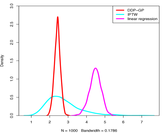
Figure 4: The density plot of estimated regime effects by DDP-GP, IPTW and linear regression in 1,000 trials.

5.3 Regime Effect for Multi-stage Regimes

Our third simulation study was designed to examine inference on strategy effects for multi-stage regimes. This simulation is a stylized version of the leukemia data that we will analyze in Section 6. We simulated samples of size $n=200$. Patients initially were randomized between two induction therapies, with the randomization probabilities based on their blood glucose values, which were simulated as $L_{i}\ \sim\ \mbox{N}(100,10^{2})$. Denoting $Z^{1}\in\{a_{1},a_{2}\}$, if $L_{i}<100$, then $Z_{i}^{1}=a_{1}$ with probability 0.6 and $Z_{i}^{1}=a_{2}$ with probability 0.4. If $L_{i}\geq 100$, then $Z_{i}^{1}=a_{1}$ with probability 0.4 and $Z_{i}^{1}=a_{2}$ with probability 0.6. We then generated a response (see below). For patients who were resistant ($R$) to their induction therapies, they were assigned salvage treatment $Z^{2,1}\in\{b_{11},b_{12}\}$. If their blood glucoses were smaller than 100, $Z^{2,1}=b_{11}$ with probability 0.8 and $Z^{2,1}=b_{12}$ with probability 0.2; if their blood glucoses were larger than 100, $Z^{2,1}=b_{11}$ with probability 0.2 and $Z^{2,1}=b_{12}$ with probability 0.8. Patients who achieved $C$ and subsequently suffered disease progression ($P$), were given salvage treatment $Z^{2,2}\in\{b_{21},b_{22}\}$. The salvage treatment for each patient $Z_{i}^{2,2}$ was assigned based on his/her baseline covariate $L_{i}$: if $L_{i}<100$, $Z_{i}^{2,2}=b_{21}$ with probability 0.2 and $Z_{i}^{2,2}=b_{22}$ with probability 0.8; if $L_{i}\geq 100$, $Z_{i}^{2,2}=b_{21}$ with probability 0.85 and $Z_{i}^{2,2}=b_{22}$ with probability 0.15. Thus, the survival time for each patient was evaluated as

$$T_{i}=\left\{\begin{array}[]{ll}T_{i}^{(0,R)}+T_{i}^{(R,D)}&\mbox{ if patient $i$ had sequence $(L,Z^{1},T^{(0,R)},Z^{2,1})$}\\ T_{i}^{(0,C)}+T_{i}^{(C,P)}+T_{i}^{(P,D)}&\mbox{ if patient $i$ had sequence $(L,Z^{1},T^{(0,C)},T^{(C,P)},Z^{2,2})$}.\end{array}\right.$$

We simulated the times of two completing risks $R$ and $C$ as $T_{i}^{(0,R)}\sim LN(\bm{\beta}^{(0,R)}\bm{x}_{i}^{(0,R)},\sigma^{(0,R)})$ and $T_{i}^{(0,C)}\sim LN(\bm{\beta}^{(0,C)}\bm{x}_{i}^{(0,C)},\sigma^{(0,C)})$, where $\bm{\beta}^{(0,R)}=(2,\,0.02,\,0)$, $\bm{\beta}^{(0,C)}=(1.5,\,0.03,\,-0.8)$, with $\bm{x}_{i}^{k}=(1,L_{i},Z_{i}^{1})$ for $k\in\{(0,R),(0,C)\}$. For transitions $k\in\{(R,D),(C,P),(P,D)\}$, we generated transition times $T_{i}^{k}\sim LN(\bm{\beta}^{k}\bm{x}_{i}^{k},\sigma^{k})$, where $\bm{\beta}^{(R,D)}=(-0.5,\,0.03,\,0.2,0.5,\,0.3)$, $\bm{\beta}^{(C,P)}=(1,\,0.05,\,1,\,-0.6)$, $\bm{\beta}^{(P,D)}=(0.8,\,0.04,\,1.5,\,-1,\,0.5,\,0.5)$, with covariate vectors
$\bm{x}_{i}^{(R,D)}=(1,\,L_{i},\,Z_{i}^{1},\log(T_{i}^{(0,R)}),Z_{i}^{2,1})$, $\bm{x}_{i}^{(C,P)}=(1,L_{i},Z_{i}^{1},\log(T_{i}^{(0,C)}))$ and $\bm{x}_{i}^{(P,D)}=(1,L_{i},Z^{1}_{i},$ $\log(T_{i}^{(0,C)}),$ $\log(T_{i}^{(C,P)}),Z^{2,2}_{i})$. We simulated $N$ = 1,000 trials with 15% censoring.

The goal is to estimate mean survival time for each DTR $(Z^{1},Z^{2,1},Z^{2,2})$. We have 8 possible DTRs in this simulation. We applied both inference under the Bayesian nonparametric DDP-GP model and IPTW to the each simulated dataset to estimate mean survival for each of the eight possible DTRs. For the nonparametric Bayesian inference we defined independent DDP-GP models $F^{k}(Y_{i}^{k}\mid\bm{x}_{i}^{k})$ for each of the $n_{T}=5$ log transition times $Y_{i}^{k}=\log T_{i}^{k}$. Figure 5 gives comparisons of the mean survival estimates using boxplots of (Estimated mean survival - Simulation truth), based on the simulation sample of 1000 datasets, obtained by DDP-GP and IPTW, for each possible DTR. The yellow boxplots represent the DDP-GP posterior mean estimates and the green boxplots represent the IPTW estimators. Figure 5 shows that the DDP-GP estimates on average are much closer to the truth and have much smaller variability, compared to the IPTW estimates, across all eight scenarios.

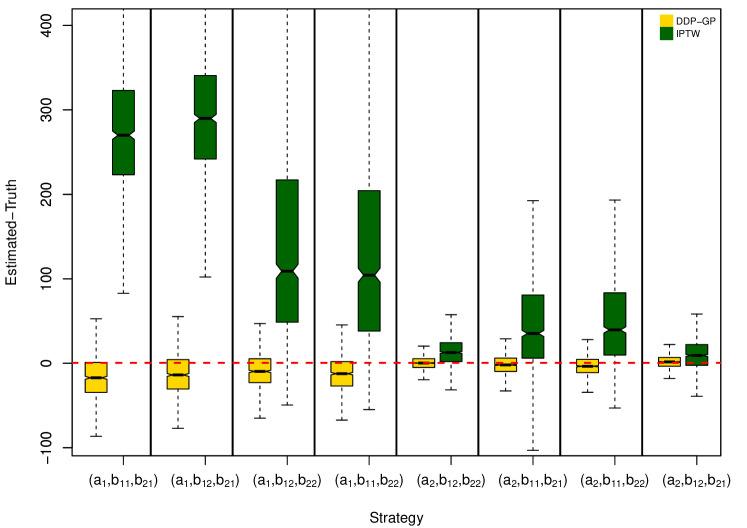
Figure 5: Simulation 3. Small (yellow) boxplots show posterior estimated OS under each of the 8 regimes as a difference with the simulation truth over 1,000 simulations. The large (green) boxes show inference under the IPTW approach. In each notched box-whisker plot, the box shows the interquartile range (IQR) from 1st quantile ($Q1$) to 3rd quantile ($Q3$), and the mid-line is the median. The top whisker denotes $Q3$+$1.5*$IQR and the bottom whisker $Q1$-$1.5*$IQR. The notch displays a confidence interval for the median, that is median$\pm 1.57*IQR/\sqrt{n}$. Here $n=1000$.

6 Evaluation of the Leukemia Trial Regimes

6.1 Computing Mean Survival Time

We first review the likelihood used by Wahed and Thall, (2013) as a basis for frequentist G-estimation of mean survival time for the leukemia trial regimes. We will apply the Bayesian nonparametric DDP-GP model to this basic structure to obtain posterior means and credible intervals of mean survival time for each DTR.

Recall that the disease states are $D$ = death, $R$ = resistant disease, $C$ = complete remission, and $P$ = progressive disease. In stage $\ell=1$ (induction chemotherapy), the three events $D,$ $R,$ and $C$ are competing risks since only one can be observed. For the $i^{th}$ patient, the stage 1 outcome is $s_{1i}=D$ if the patient dies, $s_{1i}=R$ if the patient’s disease is resistant to induction, and $s_{1i}=C$ if induction achieves CR. The corresponding transition times are $T_{i}^{(0,D)}$ = time to D (the left most arrow in Figure 1), $T_{i}^{(0,R)}$ = time to R, and $T_{i}^{(0,C)}$ = time to C. In stage 2, the transition time $T_{i}^{(R,D)}$ is defined only if $s_{1i}=R$, $T_{i}^{(C,D)}$ is defined only if $s_{1i}=C$ and $s_{2i}=D$, and $T_{i}^{(C,P)}$ is defined only if $s_{1i}=C$ and $s_{2i}=P$. The time from post-CR progression to death, $T_{i}^{(P,D)}$, is defined if $s_{1i}=C$ and $s_{2i}=P$. We thus define seven counterfactual transition times $T_{i}^{k}$, where $k$ indexes the transitions $(0,D),(0,R),(0,C),(R,D),(C,D),(C,P),(P,D)$. Figure 1 shows a flowchart of the possible outcome pathways. A dynamic treatment regime for this data may be expressed as ${\bf Z}$ = $(Z^{1},Z^{2,1},Z^{2,2})$ where $Z^{1}$ is the induction chemo, $Z^{2,1}$ is the salvage therapy given if $s_{1i}=R$, and $Z^{2,2}$ is the salvage therapy given if $s_{1i}=C$ and $s_{2i}=P.$

Our primary goal is to estimate mean survival time for each DTR $(Z^{1},Z^{2,1},Z^{2,2})$ while accounting for baseline covariates and non-random treatment assignment. Under the DDP-GP model, we denote the mean survival time for a future patient under $\bm{Z}$ by

$$\eta(\bm{Z})=E(T\mid\bm{Z}).$$ (8)

The survival time for a future patient $i=n+1$ is

$$T_{i}=I(s_{1i}=D)T_{i}^{(0,D)}+I(s_{1i}=R)(T_{i}^{(0,R)}+T_{i}^{(R,D)})\\ +I(s_{1i}=C)\{I(s_{2i}=D)(T_{i}^{(0,C)}+T_{i}^{(C,D)})+I(s_{2i}=P)(T_{i}^{(0,C)}+T_{i}^{(C,P)}+T_{i}^{(P,D)})\}.$$ (9)

The expectation of (9) under the DDP-GP model is evaluated by applying the law of total probability, using the same steps as in Wahed and Thall, (2013). We first condition on the four possible cases, $(s_{1i}=D)$, $(s_{1i}=R)$, $(s_{1i}=C,s_{2i}=D)$ and $(s_{1i}=C,s_{2i}=P)$, compute the conditional expectation in each case, and then average across the cases. This computation requires evaluating seven expressions for the conditional mean transition times

$$\eta^{k}({\bf Z},\bm{x}^{k})=E(T^{k}\mid\bm{Z},\bm{x}^{k})$$

under $F^{k}(\cdot\mid\bm{x}^{k})$, for each $k$. For example, $\eta^{(P,D)}(Z^{1},Z^{2,2},\bm{x}^{0},T^{(0,C)},T^{(C,P)})$ is the conditional mean remaining survival time, from $P$ to $D$, given that $C$ was achieved in stage 1 with frontline therapy $Z^{1}$, followed by $P$ and salvage therapy $Z^{2,2}$ in stage $2$. The DDP-GP models for $F^{k}(\cdot\mid\bm{x}^{k})$, $k=1,\ldots,n_{T}=7$ define most of the marginalization for the expectation in $\eta(\bm{Z})$, leaving only conditioning on the baseline covariates $\bm{x}_{i}^{0}$. As Wahed and Thall, (2013), we use the empirical distribution $\widehat{p}(\bm{x}^{0})$ over the observed patients to define an overall mean survival time (8). The described evaluation of $\eta(\bm{Z})$ is an application of Robins’s $G$-formula (Robins,, 1986; Robins et al.,, 2000). The complete expression is given as equation (14) in the Appendix. In the upcoming discussion we will use $\eta(\bm{Z})$ to evaluate and compare the proposed approach.

6.2 Leukemia Data – Inference for the Survival Regression

To analyze the AML-MDS trial data under the proposed DDP-GP model, we first implement posterior inference for six of the $n_{T}=7$ transition times. The exception is $T^{(C,D)}$. Due to the limited sample size – only 9 patients died after $C$ without first suffering disease progression ($P$) – we do not implement the DDP-GP model, and instead use an intercept-only Weibull AFT model. Table 1 summarizes the data. The table reports the number of patients and median transition times for some selected transitions.

We first report results for $T^{(R,D)}$. Of 210 patients, 39 (18.57%) experienced resistance to their induction therapies. The rate of resistance varied across regimes, from 31% for patients receiving FAI, 24% for FAI plus ATRA, 7.8% for FAI plus GCSF, and 10% for FAI plus ATRA plus GCSF. The times to treatment resistance were longer, with greater variability in the FAI plus GCSF arm compared to the other three arms. Among the 39 patients who were resistant to induction therapies, 27 were given HDAC as salvage treatment, of whom 2 were censored before observing death. Figure 6 summarizes survival regression under the proposed DDP-GP model by plotting posterior predicted survival functions for a hypothetical future patient at scaled age 0 with poor prognosis cytogenetic abnormality. The figure shows posterior predicted survival functions, arranged by different induction therapies $Z^{1}$ (the four curves in each panel), $T^{(0,R)}$ and $Z^{2,1}$ (as indicated in the subtitle). From Figure 6, we can see that patients with shorter $T^{(0,R)}$ have lower predicted survival once their cancer became resistant. Also, patients with $s_{1}=R$ who received $Z^{2,1}$ = HDAC as salvage had worse survival predication than patients who received salvage treatment with non HDAC. Similar results can be obtained for other transition times. Inferences for similar survival regressions for $T^{(C,P)}$ and $T^{(P,D)}$ are summarized in the on-line supplement.

	Resistance		Die after resistance
Induction	$N$	$T^{R}$(days)	Salvage	$N$	$T^{RD}$(days)
All	39	59 (47,84)	All	37	76 (27,187)
FAI	17	63 (41,97)	HDAC	25	65 (21,154)
FAI+ATRA	13	59 (55,76)
FAI+GCSF	4	77 (43.5,106.75)	non HDAC	12	146 (79, 376.75)
FAI+ATRA+GCSF	5	51 (48, 65)

	CR		Die after progression
Induction	$N$	$T^{C}$(days)	Salvage	$N$	$T^{PD}$(days)
All	102	32 (27,41)	All	83	120 (45,280)
FAI	20	31 (29, 44)	HDAC	47	106 (45,175.5)
FAI+ATRA	26	31 (25.25, 35)
FAI+GCSF	28	35.5 (28,42.75)	non HDAC	36	147.5 (42.75, 592.25)
FAI+ATRA+GCSF	28	32 (26,41)

Table 1: The sample median of each transition time is given, with lower 25% quantile and upper 75% quantile in the parenthesis next to each median .

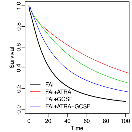
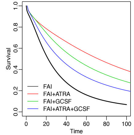
(a) $Z^{2,1}=$ HDAC, $T^{(0,R)}=20$	(b) $Z^{2,1}=$ non-HDAC, $T^{(0,R)}=20$
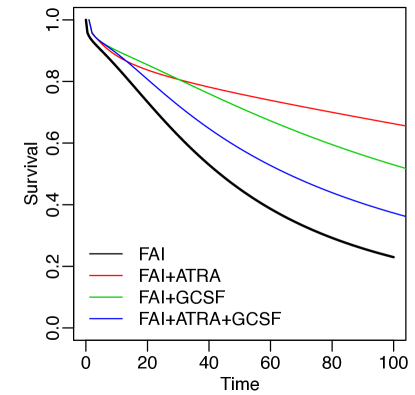
(c) $Z^{2,1}=$ HDAC; $T^{(0,R)}=55$	(d) $Z^{2,1}=$ non-HDAC; $T^{(0,R)}=55$

Figure 6: Survival regression for $T^{(R,D)}$ in the AML-MDS trial. Panels (a)-(d) show the posterior estimated survival functions for a future patient at scaled age 0 with poor prognosis cytogenetic abnormality, with $T^{(0,R)}$ and $Z^{2,1}$ as indicated. Survival curves are shown for four induction therapies. Black, red, green and blue curves indicate $Z^{1}=$ FAI, FAI+ATRA, FAI+GCSF and FAI+ATRA+GCSF, respectively.

6.3 Estimating the Regime Effects

In the AML-MDS trial, the four induction therapies and two salvage therapies define a total 16 regimes. The mean survival time estimates under each of the 16 regimes were calculated using posterior inference under independent DDP-GP models $F^{k}(Y_{i}^{k}\mid\bm{x}_{i}^{k})$ for each of the $n_{T}=7$ transition times. For comparison we also evaluated mean survival times under the IPTW method. See equation (LABEL:eq:IPTW) in the Appendix for details. Table 2 summarizes the results under IPTW and under the DDP-GP model (including 90% credible intervals). Figure (7) shows boxplots of the marginal posterior distributions of survival times under the DDP-GP model for the same 16 regimes.

Regime $(A,B_{1},B_{2})$	Estimated mean OS times (days)
	DDP-GP
	IPTW	Posterior mean	$90\%$ CI
(FAI, HDAC, HDAC)	191.67	390.35	(286.47   545.6)
(FAI, HDAC, other)	198.18	416.34	(295.84  581.73)
(FAI, other, HDAC)	216.59	394.2	(287.15  538.63)
(FAI, other, other)	222.42	420.19	(296.51  579.05)
(FAI+ATRA, HDAC, HDAC)	527.43	572.9	(416.63  829.12)
(FAI+ATRA, HDAC, other)	458.85	617.15	(434.4  905.82)
(FAI+ATRA, other, HDAC)	532.29	573.46	(413.59  830.39)
(FAI+ATRA, other, other)	464.39	617.71	(434.49  900.32)
(FAI+GCSF, HDAC, HDAC)	326.15	542.06	(393.49  725.23)
(FAI+GCSF, HDAC, other)	281.78	578.24	(419.69  781.05)
(FAI+GCSF, other, HDAC)	327.66	542.5	(392.77  726.08)
(FAI+GCSF, other, other)	283.36	578.68	(421.46   781.26)
(FAI+ATRA+GCSF, HDAC, HDAC)	337.44	458.34	(327.91  651.21)
(FAI+ATRA+GCSF, HDAC, other)	285.64	502.48	(360.29   727.44)
(FAI+ATRA+GCSF, other, HDAC)	362.56	459.42	(328.09   651.61)
(FAI+ATRA+GCSF, other, other)	309.62	503.56	(358.84  726.88)

Table 2: Mean overall survival time under the IPTW method and the posterior mean and 90% credible interval (CI) under the DDP-GP model.

Figure 7: Marginal posterior distributions of overall survival time under the DDP-GP model for all 16 regimes.

The two methods give very different estimates for mean survival time, with the DDP-GP likelihood-based estimator larger than the corresponding IPTW estimator for most regimes. The differences are expected because of the distinct properties of these two methods. The IPTW estimator uses the covariates to estimate the regime probability weights. In contrast, the DDP-GP likelihood-based method computes mean survival time, using G-estimation, accounting for patients’ covariates and previous transition times in addition to treatment followed by marginalizing over the empirical covariate distribution to obtain $\eta({\bf Z})$. Additionally, the IPTW estimate is calculated from the overall samples, whereas the likelihood-based DDP-GP method models each transition time distribution separately, which reduces the effective sample size for each model fit and thus increases the overall variability even though they share the same prior for the $\bm{\beta}^{k}$’s.

Under both methods, the estimates were smallest for the four regimes with FAI as induction therapy regardless of salvage treatment, and the 90% credible intervals were relatively small for these inferior regimes. Under the IPTW method, the estimates were largest for the four regimes with FAI plus ATRA as induction therapy, and the best regime is (FAI+ATRA, other, HDAC). With the DDP-GP likelihood-based approach, FAI plus ATRA as induction also gave the largest estimates, except for the regimes (FAI+GCSF, HDAC, other) and (FAI+GCSF, other, other), while the best regime is (FAI+ATRA, other, other). Most importantly, the DDP-GP likelihood-based approach showed that (FAI + ATRA, $Z^{2,1}$, other) was superior to (FAI + ATRA, $Z^{2,1}$, HDAC) regardless of $Z^{2,1}$. Therefore, our results suggest that (1) FAI plus ATRA was the best induction therapy, (2) if the patient’s disease was resistant to FAI plus ATRA, then it was irrelevant whether the salvage therapy contained HDAC, and (3) if patients experienced progression after achieving CR with FAI plus ATRA, then salvage therapy with non HDAC was superior.

These conclusions, although not confirmatory, are contradictory with those given by Estey et al., (1999), who concluded that none of the three adjuvant combinations FAI plus ATRA, FAI plus GCSF, or FAI plus ATRA plus GCSF were significantly different from FAI alone with respect to either survival or event-free survival time, based on consideration of only the front-line therapies by applying conventional Cox regression and hypothesis testing.

7 Conclusions

We have proposed a Bayesian nonparametric DDP-GP model for analyzing survival data and evaluating joint effects of induction-salvage therapies in clinical trials, using the posterior estimates, to predict survival for future patients. The Bayesian paradigm works very well, and the simulation studies suggest that our DDP-GP method yields more reliable estimates than IPTW.

We employed two different methods to evaluate the 16 possible two-stage regimes for choosing induction and salvage therapies in the leukemia trial data. The IPTW method estimates the regime effect by using covariates only to compute the assignment probabilities of salvage therapies to correct for bias. In contrast, likelihood-based G-estimation under the DDP-GP model accounts for all possible outcome paths, the transition times between successive states, and effects of covariates and previous outcomes, on each transition time. Although the two methods gave different numerical estimates of mean survival time, they both reached the conclusion that FAI plus ATRA was the best induction therapy and FAI was the worst induction therapy. Although our current models are set up for two-stage treatment regimes, they easily can be extended to other applications with multi-stage regimes.

Appendix

The following structure is that given by Wahed and Thall, (2013), and is included here for completeness. The risk sets of the seven transition time in the leukemia trial are defined as follows. Let $G^{0}=\{1,\ldots,n\}$ denote the initial risk set at the start of induction chemotherapy, and $G^{(0,r)}=\{i:\;s_{1i}=r\}$ for $r=D,C,R$, so $G^{0}$ = $G^{(0,D)}\cup G^{(0,C)}\cup G^{(0,R)}$. Similarly, $G^{(C,P)}=\{i:\;s_{1i}=C,s_{2i}=P\}$ is the later risk set for $T^{(P,D)}$.

To record right censoring, let $U_{i}$ denote the time from the start of induction to last followup for patient $i$. We assume that $U_{i}$ is conditionally independent of the transition times given prior transition times and other covariates. Censoring of event times occurs by competing risk and/or loss to follow up. For a patient $i$ in the risk set for event time $T^{k}_{i}$, let $\delta_{i}^{k}$ = 1 if a patient $i$ is not censored and 0 if patient $i$ is right censored. For example, $\delta_{i}^{(0,D)}=1$ for $i\in G^{0}$ if $T_{i}^{(0,D)}=\min(U_{i},T_{i}^{(0,k)},k=D,C,R)$. Similarly, $\delta_{i}^{(R,D)}=1$ for $i\in G^{(0,R)}$ if $T_{i}^{(0,R)}+T_{i}^{(R,D)}<U_{i}$ and $\delta_{i}^{(P,D)}=1$ for $i\in G^{(C,P)}$ if $T_{i}^{(0,C)}+T_{i}^{(C,P)}+T_{i}^{(P,D)}<U_{i}$.

Let $V_{x,i}$ denote the observed time for patient $i$ in risk set $G^{x}$, as follows. For $i\in G^{0}$ let $V_{1,i}=\min(T^{(0,D)}_{i},T^{(0,R)}_{i},T^{(0,C)}_{i},U_{i})$ denote the observed time for the stage 1 event or censoring. For $i\in G^{(0,C)}$ let $V_{Ci}=\min(T^{(C,D)}_{i},T^{(C,P)}_{i},U_{i}-T^{(0,C)}_{i})$ denote the observed event time for the competing risks $D$ and $P$ and loss to followup. Similarly, for $i\in G^{(0,R)}$, let $V_{Ri}=\min(T^{(R,D)}_{i},U_{i}-T^{(R,D)}_{i})$, and for $i\in G^{(C,P)}$ let $V_{(C,P),i}=\min(T^{(P,D)}_{i},U_{i}-T^{(0,C)}_{i}-T^{(C,P)}_{i})$.

The joint likelihood function is the product ${\cal L}\ =\ {\cal L}_{1}{\cal L}_{2}{\cal L}_{3}{\cal L}_{4}.$ The first factor ${\cal L}_{1}$ corresponds to response to induction therapy,

$${\cal L}_{1}=\prod_{i\in G^{0}}\prod_{k\in\{D,R,C\}}f^{(0,k)}(V_{1,i}\mid\bm{x}^{k}_{i})^{\delta^{(0,k)}_{i}}S^{(0,k)}(V_{1,i}\mid\bm{x}^{k}_{i})^{1-\delta^{(0,k)}_{i}}.$$ (10)

where $S^{k}$ = $1-F^{k}.$ The second factor ${\cal L}_{2}$ corresponds to patients $i\in G^{(0,R)}$ who experience resistance to induction and receive salvage $Z^{2,1}$,

$${\cal L}_{2}=\prod_{i\in G^{(0,R)}}f^{(R,D)}(V_{Ri}\mid\bm{x}^{(R,D)}_{i})^{\delta^{(R,D)}_{i}}S^{(R,D)}(V_{Ri}\mid\bm{x}_{i}^{(R,D)})^{1-\delta^{(R,D)}_{i}}.$$ (11)

The third factor ${\cal L}_{3}$ is the likelihood contribution from patients achieving CR,

$${\cal L}_{3}=\prod_{i\in G^{(0,C)}}\;\;\prod_{k=(C,D),(C,P)}f^{k}(V_{Ci}\mid\bm{x}^{k}_{i})^{\delta^{k}_{i}}S^{k}(V_{Ci}\mid\bm{x}^{k}_{i})^{1-\delta^{k}_{i}}.$$ (12)

The fourth factor ${\cal L}_{4}$ is the contribution from patients who experience tumor progression after CR

$${\cal L}_{4}=\prod_{i\in G^{(C,P)}}f^{(P,D)}(V_{CP,i}\mid\bm{x}^{(P,D)}_{i})^{\delta^{(P,D)}_{i}}\,S^{(P,D)}(V_{CP,i}\mid\bm{x}^{(P,D)}_{i})^{1-\delta^{(P,D)}_{i}}.$$ (13)

The mean survival time of a patient treated with regime ${\bf Z}$ = $(Z^{1},Z^{2,1},Z^{2,2})$ is

$$\eta({\bf Z})=\int\Big{[}p(s_{1}=D\mid\bm{x}^{0},Z^{1})\eta^{(0,D)}(\bm{x}^{0},Z^{1})\Big{]}d\widehat{p}(\bm{x}^{0})\\ +\int\Big{\{}p(s_{1}=R\mid\bm{x}^{0},Z^{1})\Big{[}\eta^{R}(\bm{x}^{0},Z^{1})+\int\eta^{(R,D)}(\bm{x}^{0},Z^{1},Z^{2,1},T^{(0,R)})d\mu(T^{(0,R)})\Big{]}\Big{\}}d\widehat{p}(\bm{x}^{0})\\ +\int p(s_{1}=C\mid\bm{x}^{0},Z^{1})\Big{[}\eta^{C}(\bm{x}^{0},Z^{1})+\int\Big{[}p(s_{2}=D\mid s_{1}=C,\bm{x}^{0},Z^{1},T^{(0,C)})\eta^{(C,D)}(\bm{x}^{0},Z^{1},T^{C})\\ +p(s_{2}=P\mid s_{1}=C,\bm{x}^{0},Z^{1},T^{(0,C)})[\eta^{(C,P)}(\bm{x}^{0},Z^{1},T^{(0,C)})\\ +\int\eta^{(P,D)}(\bm{x}^{0},Z^{1},Z^{2,2}T^{(0,C)},T^{(C,P)})d\mu(T^{(C,P)})]d\mu(T^{(0,C)})\Big{]}d\widehat{p}(\bm{x}^{0}).$$ (14)

We compute the IPTW estimates for overall mean survival with regime ${\bf Z}$ as

$$IPTW({\bf Z})=\sum_{i=1}^{n}\,w_{i}({\bf Z})T_{i}\ /\ \sum_{i=1}^{n}\,w_{i}({\bf Z}),$$ (15)

where

$$w_{i}({\bf Z}) = \frac{I({\bf Z}={\bf Z}_{i})\delta_{i}}{\hat{K}(U_{i})}\biggl{[}I(s_{1i}=D)+I(s_{1i}=R)I_{i}(Z^{2,1})/\hat{\mathrm{Pr}}(Z^{2,1}\mid s_{1i}=R,Z^{1},\bm{x}^{0}_{i},T_{i}^{(0,R)})$$

$$+I(s_{1i}=C,s_{2i}=D)$$

$$+I(s_{1i}=C,s_{2i}=P)I_{i}(Z^{2,2})/\hat{\mathrm{Pr}}(Z^{2,2}\mid s_{1i}=C,s_{2i}=P,Z^{1},\bm{x}_{i}^{0},T_{i}^{(0,C)},T_{i}^{(C,P)})\biggr{]}.$$

In (LABEL:eq:IPTW), $\hat{K}$ is the Kaplan-Meier estimator of the censoring survival distribution $K(u)=P(U\geq t)$ at time $t$. $I_{i}(Z)$ is is an indictor of treatment $Z$ and 0 otherwise, and $\hat{\mathrm{Pr}}(Z^{2,1}\mid s_{1i}=C,Z^{1},\bm{x}^{0}_{i},T_{i}^{(0,R)})$ is the probability of receiving salvage treatment $Z^{2,1}$ estimated using logistic regression, and similarly for $\hat{\mathrm{Pr}}(Z^{2,2}\mid s_{1i}=C,s_{2i}=P,Z^{1},\bm{x}^{0}_{i},T_{i}^{(0,C)},T_{i}^{(C,P)})$. The above estimator has been shown to be consistent under suitable assumptions (Wahed and Thall,, 2013; Scharfstein et al.,, 1999).

References

- Bernardo et al., (1999) Bernardo, J., Berger, J., and Smith, A. D. F. (1999). Regression and classification using gaussian process priors. In Bayesian Statistics 6: Proceedings of the Sixth Valencia International Meeting, June 6-10, 1998, volume 6, page 475. Oxford University Press.
- Connolly and Bernstein, (2007) Connolly, S. and Bernstein, G. (2007). Practice parameter for the assessment and treatment of children and adolescents with anxiety disorders. Journal of the American Academy of Child and Adolescent Psychiatry, 46(2):267–283.
- Dawson and Lavori, (2004) Dawson, R. and Lavori, P. W. (2004). Placebo-free designs for evaluating new mental health treatments: the use of adaptive treatment strategies. Statistics in medicine, 23(21):3249–3262.
- Estey et al., (1999) Estey, E. H., Thall, P. F., Pierce, S., Cortes, J., Beran, M., Kantarjian, H., Keating, M. J., Andreeff, M., and Freireich, E. (1999). Randomized phase ii study of fludarabine+ cytosine arabinoside+ idarubicinall-trans retinoic acidgranulocyte colony-stimulating factor in poor prognosis newly diagnosed acute myeloid leukemia and myelodysplastic syndrome. Blood, 93(8):2478–2484.
- Ferguson, (1973) Ferguson, T. S. (1973). A bayesian analysis of some nonparametric problems. The annals of statistics, pages 209–230.
- Hernán et al., (2000) Hernán, M. Á., Brumback, B., and Robins, J. M. (2000). Marginal structural models to estimate the causal effect of zidovudine on the survival of hiv-positive men. Epidemiology, 11(5):561–570.
- Hill, (2011) Hill, J. L. (2011). Bayesian nonparametric modeling for causal inference. Journal of Computational and Graphical Statistics, 20(1).
- Ishwaran and James, (2001) Ishwaran, H. and James, L. F. (2001). Gibbs sampling methods for stick-breaking priors. Journal of the American Statistical Association, 96(453).
- Karabatsos and Walker, (2012) Karabatsos, G. and Walker, S. G. (2012). A bayesian nonparametric causal model. Journal of Statistical Planning and Inference, 142(4):925–934.
- Lavori and Dawson, (2000) Lavori, P. W. and Dawson, R. (2000). A design for testing clinical strategies: biased adaptive within-subject randomization. Journal of the Royal Statistical Society: Series A (Statistics in Society), 163(1):29–38.
- Lunceford et al., (2002) Lunceford, J. K., Davidian, M., and Tsiatis, A. A. (2002). Estimation of survival distributions of treatment policies in two-stage randomization designs in clinical trials. Biometrics, 58(1):48–57.
- MacEachern, (1999) MacEachern, S. N. (1999). Dependent nonparametric processes. In ASA proceedings of the section on bayesian statistical science, pages 50–55. American Statistical Association, pp. 50–55, Alexandria, VA.
- MacEachern and Müller, (1998) MacEachern, S. N. and Müller, P. (1998). Estimating mixture of dirichlet process models. Journal of Computational and Graphical Statistics, 7(2):223–238.
- Moodie et al., (2007) Moodie, E. E., Richardson, T. S., and Stephens, D. A. (2007). Demystifying optimal dynamic treatment regimes. Biometrics, 63(2):447–455.
- Müller and Mitra, (2013) Müller, P. and Mitra, R. (2013). Bayesian nonparametric inference–why and how. Bayesian Analysis, 8(2):269–302.
- Müller and Rodriguez, (2013) Müller, P. and Rodriguez, A. (2013). Nonparametric bayesian inference. IMS-CBMS Lecture Notes. IMS, 270.
- Murphy et al., (2001) Murphy, S., Van Der Laan, M., and Robins, J. (2001). Marginal mean models for dynamic regimes. Journal of the American Statistical Association, 96(456):1410–1423.
- Murphy, (2003) Murphy, S. A. (2003). Optimal dynamic treatment regimes. Journal of the Royal Statistical Society: Series B (Statistical Methodology), 65(2):331–355.
- Murphy, (2005) Murphy, S. A. (2005). An experimental design for the development of adaptive treatment strategies. Statistics in medicine, 24(10):1455–1481.
- (20) Murphy, S. A., Collins, L. M., and Rush, A. J. (2007a). Customizing treatment to the patient: adaptive treatment strategies. Drug and alcohol dependence, 88(Suppl 2):S1–3.
- (21) Murphy, S. A., Lynch, K. G., Oslin, D., McKay, J. R., and TenHave, T. (2007b). Developing adaptive treatment strategies in substance abuse research. Drug and alcohol dependence, 88:S24–S30.
- Neal, (1995) Neal, R. (1995). Bayesian Learning for Neural Networks. PhD thesis, Graduate Department of Computer Science, University of Toronto.
- Neal, (2000) Neal, R. M. (2000). Markov chain sampling methods for dirichlet process mixture models. Journal of computational and graphical statistics, 9(2):249–265.
- O’Hagan and Kingman, (1978) O’Hagan, A. and Kingman, J. (1978). Curve fitting and optimal design for prediction. Journal of the Royal Statistical Society. Series B (Methodological), 40(1):1–42.
- Rasmussen and Williams, (2006) Rasmussen, C. and Williams, C. (2006). Gaussian Processes for Machine Learning. ISBN 0-262-18253-X. MIT Press.
- Robins, (1986) Robins, J. (1986). A new approach to causal inference in mortality studies with a sustained exposure period?application to control of the healthy worker survivor effect. Mathematical Modelling, 7(9):1393–1512.
- Robins et al., (2008) Robins, J., Orellana, L., and Rotnitzky, A. (2008). Estimation and extrapolation of optimal treatment and testing strategies. Statistics in medicine, 27(23):4678–4721.
- Robins, (1987) Robins, J. M. (1987). Addendum to ?a new approach to causal inference in mortality studies with a sustained exposure period?application to control of the healthy worker survivor effect? Computers & Mathematics with Applications, 14(9):923–945.
- Robins, (1989) Robins, J. M. (1989). The analysis of randomized and non-randomized aids treatment trials using a new approach to causal inference in longitudinal studies. Health service research methodology: a focus on AIDS, 113:159.
- Robins, (1997) Robins, J. M. (1997). Causal inference from complex longitudinal data. In Latent variable modeling and applications to causality, pages 69–117. Springer.
- Robins, (2004) Robins, J. M. (2004). Optimal structural nested models for optimal sequential decisions. In Proceedings of the Second Seattle Symposium in Biostatistics, pages 189–326. Springer.
- Robins et al., (2000) Robins, J. M., Hernán, M. Á., and Brumback, B. (2000). Marginal structural models and causal inference in epidemiology. Epidemiology, 11(5):550–560.
- Robins and Rotnitzky, (1992) Robins, J. M. and Rotnitzky, A. (1992). Recovery of information and adjustment for dependent censoring using surrogate markers. In AIDS Epidemiology, pages 297–331. Springer.
- Scharfstein et al., (1999) Scharfstein, D. O., Rotnitzky, A., and Robins, J. M. (1999). Adjusting for nonignorable drop-out using semiparametric nonresponse models. Journal of the American Statistical Association, 94(448):1096–1120.
- Sethuraman, (1991) Sethuraman, J. (1991). A constructive definition of dirichlet priors. Technical report, DTIC Document.
- Shi et al., (2007) Shi, J. Q., Wang, B., Murray-Smith, R., and Titterington, D. M. (2007). Gaussian process functional regression modeling for batch data. Biometrics, 63(3):714–723.
- (37) Thall, P. F., Logothetis, C., Pagliaro, L. C., Wen, S., Brown, M. A., Williams, D., and Millikan, R. E. (2007a). Adaptive therapy for androgen-independent prostate cancer: a randomized selection trial of four regimens. Journal of the National Cancer Institute, 99(21):1613–1622.
- Thall et al., (2000) Thall, P. F., Millikan, R. E., Sung, H.-G., et al. (2000). Evaluating multiple treatment courses in clinical trials. Statistics in Medicine, 19(8):1011–1028.
- Thall et al., (2002) Thall, P. F., Sung, H.-G., and Estey, E. H. (2002). Selecting therapeutic strategies based on efficacy and death in multicourse clinical trials. Journal of the American Statistical Association, 97(457).
- (40) Thall, P. F., Wooten, L. H., Logothetis, C. J., Millikan, R. E., and Tannir, N. M. (2007b). Bayesian and frequentist two-stage treatment strategies based on sequential failure times subject to interval censoring.
- van der Laan and Petersen, (2007) van der Laan, M. J. and Petersen, M. L. (2007). Causal effect models for realistic individualized treatment and intention to treat rules. International Journal of Biostatistics, 3(1):3.
- Wahed and Thall, (2013) Wahed, A. S. and Thall, P. F. (2013). Evaluating joint effects of induction–salvage treatment regimes on overall survival in acute leukaemia. Journal of the Royal Statistical Society: Series C (Applied Statistics), 62(1):67–83.
- Wahed and Tsiatis, (2006) Wahed, A. S. and Tsiatis, A. A. (2006). Semiparametric efficient estimation of survival distributions in two-stage randomisation designs in clinical trials with censored data. Biometrika, 93(1):163–177.
- Wang et al., (2012) Wang, L., Rotnitzky, A., Lin, X., Millikan, R. E., and Thall, P. F. (2012). Evaluation of viable dynamic treatment regimes in a sequentially randomized trial of advanced prostate cancer. Journal of the American Statistical Association, 107(498):493–508.
- Williams, (1998) Williams, C. (1998). Prediction with gaussian processes: From linear regression to linear prediction and beyond. NATO ASI SERIES D BEHAVIOURAL AND SOCIAL SCIENCES, 89:599–621.