Orbital ferromagnetism in interacting few-electron dots with strong spin-orbit coupling

Abstract

We study the ground state of $N$ weakly interacting electrons (with $N\leq 10$) in a two-dimensional parabolic quantum dot with strong Rashba spin-orbit coupling. Using dimensionless parameters for the Coulomb interaction, $\lambda\lesssim 1$, and the Rashba coupling, $\alpha\gg 1$, the low-energy physics is characterized by an almost flat single-particle dispersion. From an analytical approach for $\alpha\to\infty$ and $N=2$, and from numerical exact diagonalization and Hartree-Fock calculations, we find a transition from a conventional unmagnetized ground state (for $\lambda<\lambda_{c}$) to an orbital ferromagnet (for $\lambda>\lambda_{c}$), with a large magnetization and a circulating charge current. We show that the critical interaction strength, $\lambda_{c}=\lambda_{c}(\alpha,N)$, vanishes in the limit $\alpha\to\infty$.

I Introduction

The electronic properties of few-electron quantum dots in semiconductor nanostructures have been widely studied over the past decades nazarov ; reimann ; kouwenhoven . Typically, electrons in the two-dimensional (2D) electron gas formed at the interface between different semiconductor layers are confined to a localized region in space by means of electrostatic trapping. The resulting confinement is usually well approximated by a parabolic potential with oscillator frequency $\omega$, suggesting a simple 2D oscillator spectrum. However, Coulomb interactions are important in such devices, and their impact can readily be seen in transport spectroscopy kouwenhoven . Apart from the ubiquitous Coulomb charging effects, they are also predicted to induce a transition to a finite-size Wigner crystal of $N$ electrons, the “Wigner molecule” egger ; landman , where the electrostatic repulsion suppresses quantum fluctuations and inter-electron distances are maximized jauregui ; peeters ; peeters2 . The ratio between the confinement scale, $l_{T}=\sqrt{\hbar/m_{e}\omega}$, with the effective mass $m_{e}$, and the Bohr radius, $a_{B}=\hbar^{2}\varepsilon_{0}/m_{e}e^{2}$, defines a dimensionless interaction strength parameter reimann ,

$$\lambda=\frac{l_{T}}{a_{B}}=\frac{e^{2}}{\varepsilon_{0}\hbar\omega l_{T}}.$$ (1)

Interactions are here described by the standard Coulomb potential, $V({\bf r})=e^{2}/\varepsilon_{0}r$, where the dielectric constant $\varepsilon_{0}$ accounts for static external screening. The crossover from the weakly interacting Fermi liquid phase (realized for $\lambda\ll 1$) to the Wigner molecule then happens around $\lambda\approx 1$ and is known to be rather sharp despite of the finite-size geometry egger . Due to the confinement-induced reduction of quantum fluctuations, the corresponding electron densities near the transition are much higher than the one required for bulk Wigner crystal formation reimann .

Another modification of the 2D oscillator spectrum is caused by spin-orbit coupling. We here focus on the Rashba term caused by interface electric fields, which often is the dominant spin-orbit coupling and can be tuned by gate voltages winkler . Other types of spin-orbit coupling are expected to generate similar physics as described below, assuming that one can reach the corresponding strong-coupling regime. In particular, the model studied below applies directly to the case of Dresselhaus spin-orbit coupling winkler . With the Rashba wavenumber $k_{0}$, it is convenient to employ a dimensionless Rashba coupling,

$$\alpha=k_{0}l_{T}=k_{0}\sqrt{\frac{\hbar}{m_{e}\omega}}.$$ (2)

The single-particle spectrum of a dot with weak Rashba coupling, $\alpha\lesssim 1$, has been discussed, e.g., in Refs. tretyak ; tapash . Interaction effects in few-electron dots with $\alpha\lesssim 1$ have been investigated by density functional theory governale , quantum Monte Carlo simulations pede ; weissegger ; pederiva , exact diagonalization ulloa0 ; ulloa ; chakra , and configuration interaction calculations cavalli . With increasing $\alpha$, the Wigner molecule transition was found to shift to weaker interactions, i.e., to smaller $\lambda$. As noted in Refs. kivelson ; silvestrov , the related bulk Wigner crystal formation is also easier to achieve when the Rashba term is present.

In this paper, we study interacting few-electron quantum dots in the regime of large Rashba spin-orbit coupling, $\alpha\gg 1$. This regime appears to be within close experimental reach nitta ; ensslin ; ast0 ; ast1 ; ast2 ; aruga ; tarucha ; murakawa , and is also of considerable fundamental interest. In fact, many materials with strong spin-orbit coupling are known to realize a topological insulator phase hasan ; qi . Near the boundary of a noninteracting 2D topological insulator with time reversal symmetry (TRS), an odd number of gapless one-dimensional (1D) helical edge states must be present hasan ; qi , where the spin is tied to the momentum of the electron. As we do not address magnetic field effects here, the Hamiltonian below enjoys TRS. Moreover, it is characterized by strong spin-orbit coupling, and it resembles a topological insulator in the absence of interactions.

Given the above developments, it is not surprising that several theoretical works li1 ; li2 ; rashba ; ghosh ; sherman have already addressed the physics of noninteracting electrons in quantum dots with $\alpha\gg 1$. In this limit, the low-energy spectrum of a parabolic dot is well described by a sequence of almost flat Landau-like bands (see Sec. II.1),

$$E_{J,n}\simeq\hbar\omega\left(n+\frac{1}{2}+\frac{J^{2}}{2\alpha^{2}}\right),$$ (3)

with half-integer total angular momentum $J$ and the band index $n=0,1,2,\ldots$, such that states with the same $n$ but different $J$ are almost degenerate. Equation (3) reflects the spectrum of a 1D (radial) oscillator plus a decoupled rotor with large moment of inertia. Assuming that the Fermi energy is within the $n=0$ band, with corresponding Fermi angular momentum $J_{F}$, the Kramers pair with $J=\pm J_{F}$ has eigenfunctions localized near the “edge” of the dot. In fact, those states have the largest distance from the dot center among all occupied states, and form a helical edge with opposite spin orientation of the counterpropagating $\pm J_{F}$ states li1 . By virtue of the bulk-boundary correspondence hasan , the authors of Ref. li1 argued that a noninteracting dot with $\alpha\gg 1$ has features similar to the finite-size version of a 2D topological insulator. Indeed, time reversal invariant single-particle perturbations, e.g., representing the effects of elastic disorder, are predicted not to mix opposite-spin states, and the helical edge is therefore protected against such sources of backscattering. In the finite-size dot geometry, however, the $\mathbb{Z}_{2}$ invariant commonly employed to classify the topological insulator phase is not well defined.

For a dot with $\alpha\gg 1$, since the noninteracting spectrum is almost flat, one can expect that interactions have a profound effect. For instance, in lattice models hosting a topological insulator phase for weak interactions, Mott insulator or spin liquid phases emerge for strong interactions balents ; for the case of interacting bosons, see Refs. atoms1 ; atoms2 ; atoms3 ; atoms4 ; atoms5 . Moreover, the conspiracy of a single-particle potential with sufficiently strong Coulomb interactions can induce two-particle Umklapp processes destroying the helical edge state xumoore ; wuzhang . Motivated by these developments, we here study the ground state of interacting electrons in a quantum dot with strong Rashba spin-orbit coupling. We find it quite remarkable that the relatively simple Hamiltonian below captures such diverse behaviors as Wigner molecule formation, the presence of helical edge states, and – as we shall argue – the molecular equivalent of an orbital ferromagnet. This Hamiltonian is also expected to accurately describe semiconductor experiments, where recent progress holds promise of reaching the ultra-strong Rashba coupling regime. Let us now briefly summarize our main results, along with a description of the structure of the paper.

In Sec. II.1, we present the single-particle model for the quantum dot, and summarize its solution for large Rashba parameter $\alpha$. While our general conclusions hold for arbitrary radially symmetric confinement, quantitative results are provided for the most important case of a parabolic trap. We introduce a single-band approximation valid for weak-to-intermediate interaction strength, $\lambda\lesssim 1$, and energy scales below $\hbar\omega$, which allows one to make significant analytical progress. In Sec. II.2, we then discuss the general properties of Coulomb matrix elements. The limit of ultra-strong Rashba coupling, $\alpha\to\infty$, is addressed in Sec. II.3, where a simple analytical result for the Coulomb matrix elements is derived. For the resulting $\alpha\to\infty$ model, $H_{\infty}$, already weak interactions induce strongly correlated phases. The Coulomb matrix elements not included in $H_{\infty}$, arising for large but finite $\alpha$, are addressed in detail in Sec. II.4.

Next, in Sec. III, we present the exact ground-state solution of $H_{\infty}$ for two electrons ($N=2$). While the above discussion may suggest that a Wigner molecule will be formed, we find an orbital ferromagnetic state. The $N=2$ ground state of $H_{\infty}$, see Sec. III.1, is shown to be highly degenerate in Sec. III.2. However, perturbative inclusion of Coulomb corrections beyond $H_{\infty}$, see Sec. III.3, breaks the degeneracy and suggest the possibility of spontaneously broken TRS in an interacting $N=2$ dot (for a more precise characterization of this phenomenon, see Sec. III), with a large value of the total angular momentum found already for weak interactions. The emergence of a finite magnetization foot01 , $M_{s}\neq 0$, suggests a finite-size (“molecular”) version of an orbital ferromagnet. This remarkable behavior appears at arbitrarily weak (but finite) interaction strength, with giant values of the magnetization. We estimate $M_{s}\approx(\lambda\alpha)^{1/4}\hbar$, see Sec. III.3. This highlights that the orbital angular momentum is behind this phenomenon, see also Ref. hernando .

In Sec. IV.1, we then present exact diagonalization results for the ground-state energy of $N=2$ and $N=3$ electrons in the dot for $\alpha=10$ and $\alpha=15$, going beyond the $\alpha\to\infty$ model $H_{\infty}$. We now find that only above a critical interaction strength, $\lambda>\lambda_{c}(\alpha,N)$, the dot develops a magnetization, $M_{s}\neq 0$. The parameter $\lambda_{c}$ becomes smaller with increasing $\alpha$, which is consistent with $\lambda_{c}(\alpha\to\infty)\to 0$ as obtained from $H_{\infty}$ in Sec. III. In Sec. IV.2, we then discuss Hartree-Fock (HF) results for particle numbers up to $N=10$, where exact diagonalization becomes computationally too expensive. The HF results show qualitatively the same effects, indicating that orbital ferromagnetism represents the generic behavior of weakly interacting electrons in quantum dots with ultra-strong Rashba coupling. Finally, we conclude in Sec. V, where we also discuss perspectives for experiments. Additional details about the $\alpha\to\infty$ limit are given in an Appendix.

II Coulomb interactions in a Rashba dot

II.1 Single particle problem

We consider electrons in a 2D quantum dot with parabolic confinement in the $xy$ plane. Including the Rashba spin-orbit coupling, the single-particle Hamiltonian reads winkler

$$H_{\rm dot}=\frac{\hbar^{2}}{2m_{e}}{\bf k}^{2}+\frac{m_{e}}{2}\omega^{2}{\bf r}^{2}-\frac{\hbar^{2}k_{0}k}{m_{e}}{\cal P}_{h},$$ (4)

where ${\bf k}=-i(\partial_{x},\partial_{y})$, ${\bf r}=(x,y)$, $\omega$ is the trap frequency (defined in the absence of spin-orbit coupling), and the positive wavenumber $k_{0}$ determines the Rashba coupling. With Pauli matrices $\sigma_{x,y,z}$ referring to the electronic spin, the Hermitian helicity operator, ${\cal P}_{h}=(k_{y}\sigma_{x}-k_{x}\sigma_{y})/k$, has the eigenvalues $\pm 1$. In the absence of the trap ($\omega=0$), helicity and momentum are conserved quantities. Writing ${\bf k}=k(\cos\phi,\sin\phi)$, it is a simple exercise to obtain the ${\cal P}_{h}$-eigenspinors, $\Phi_{\pm}(\phi)$, with conserved helicity $\pm 1$. The dispersion relation is then (up to a constant shift) given by $\hbar^{2}(k\mp k_{0})^{2}/2m_{e}$. Low-energy states have positive helicity with

$$\Phi_{+}(\phi)=\frac{1}{\sqrt{2}}\left(\begin{array}[]{c}1\\ -ie^{i\phi}\end{array}\right),$$ (5)

and for given $k\approx k_{0}$, a U(1) degeneracy is realized, corresponding to a ring in momentum space.

In the presence of the trap, however, helicity and momentum are not conserved anymore. The system now has two characteristic length scales, namely the confinement scale, $l_{T}=\sqrt{\hbar/m_{e}\omega}$, and the spin-orbit length, $1/k_{0}$. Their ratio determines the dimensionless Rashba parameter $\alpha$ in Eq. (2). In this paper, we discuss the case $\alpha\gg 1$, where positive helicity states are separated from ${\cal P}_{h}=-1$ states by a huge gap of order $\hbar^{2}k_{0}^{2}/m_{e}=\alpha^{2}\hbar\omega$. As a consequence, negative helicity states can safely be projected away. Noting that the total angular momentum operator, $J_{z}=-i\hbar\partial_{\phi}+\hbar\sigma_{z}/2$, is conserved, with eigenvalues $\hbar J$ (half-integer $J$), the low-energy eigenstates of $H_{\rm dot}$ for $\alpha\gg 1$ have the momentum representation

$$\psi_{J,n}(\kappa,\phi)=\frac{e^{i(J-1/2)\phi}}{\sqrt{2\pi\kappa}}\ u_{J,n}(\kappa)\Phi_{+}(\phi),$$ (6)

where we use the dimensionless positive wavenumber $\kappa=kl_{T}$. The radial wavefunction, $u_{J,n}(\kappa)$, obeys the effective 1D Schrödinger equation li1 ; ghosh

$$\left(-\frac{1}{2}\partial_{\kappa}^{2}+\frac{1}{2}(\kappa-\alpha)^{2}+\frac{J^{2}}{2\kappa^{2}}-\frac{E_{J,n}}{\hbar\omega}\right)u_{J,n}(\kappa)=0,$$ (7)

where $n=0,1,2,\ldots$ labels the solutions. For $\alpha\gg 1$, it is justified to approximate Eq. (7) by replacing $J^{2}/2\kappa^{2}\to J^{2}/2\alpha^{2}$. The radial problem then decouples from the angular one and becomes equivalent to a shifted 1D oscillator with energy levels $(n+1/2)\hbar\omega$. Moreover, the angular problem reduces to a rigid rotor with the large moment of inertia $\alpha^{2}/\hbar\omega$. We thus arrive at the $E_{J,n}$ quoted in Eq. (3), where $n$ serves as band index and $J$ labels the almost degenerate states within each band. We find that corrections to the energies in Eq. (3) scale $\sim 1/\alpha^{3}$ for $\alpha\gg 1$. In fact, a recent numerical study of $H_{\rm dot}$ has reported that Eq. (3) is highly accurate for $\alpha\gtrsim 4$ ghosh .

For weak-to-intermediate Coulomb interaction strength, only low-energy states are needed to span the effective Hilbert space determining the ground state. It can then be justified to retain only $n=0$ modes. This step implies the restriction to angular momentum states with $|J|\lesssim\alpha$, since otherwise $n>0$ states should also be included. For the results below, we have checked that this “single-band approximation” is indeed justified. From now on, the single-particle Hilbert space is restricted to the $n=0$ sector (and the $n$ index will be dropped). In momentum representation, this space is spanned by the orthonormal set of states footnew

$$\psi_{J}(\kappa,\phi)=\frac{\pi^{1/4}l_{T}}{\sqrt{\kappa}}e^{-(\kappa-\alpha)^{2}/2}e^{i(J-1/2)\phi}\left(\begin{array}[]{c}1\\ -ie^{i\phi}\end{array}\right).$$ (8)

Up to the zero-point contribution, the corresponding single-particle energy is $E_{J}=J^{2}\hbar\omega/2\alpha^{2}$. The momentum-space probability density for all states is independent of $J$, representing a radially symmetric Gaussian peak centered at $k=k_{0}$,

$$\rho_{J}(k)=|\psi_{J}|^{2}=\frac{2\sqrt{\pi}l_{T}}{k}e^{-(k-k_{0})^{2}l_{T}^{2}}.$$ (9)

The coordinate representation of Eq. (8) now follows by Fourier transformation,

$$\tilde{\psi}_{J}(\rho,\theta)=\frac{i^{J-1/2}}{l_{T}}e^{i(J-1/2)\theta}\left(\begin{array}[]{c}F_{J-1/2}(\rho)\\ e^{i\theta}F_{J+1/2}(\rho)\end{array}\right),$$ (12)

$$F_{m}(\rho)=\int_{0}^{\infty}\frac{d\kappa\sqrt{\kappa}}{2\pi^{3/4}}e^{-(\kappa-\alpha)^{2}/2}J_{m}(\kappa\rho),$$ (13)

where ${\bf r}=r(\cos\theta,\sin\theta)$ with $\rho=r/l_{T}$, and we use the Bessel functions $J_{m}(x)$ (integer $m$).

It will be convenient to use a second-quantized formalism below, with the noninteracting Hamiltonian

$$H_{0}=\sum_{J}E_{J}c_{J}^{\dagger}c_{J},\quad E_{J}=\frac{J^{2}}{2\alpha^{2}}\hbar\omega,$$ (14)

where fermion annihilation operators are denoted by $c_{J}$ for half-integer $J$. The electron field operator is then given by

$$\Psi({\bf r})=\sum_{J}\tilde{\psi}_{J}({\bf r})c_{J}.$$ (15)

The noninteracting ground state is a Fermi sea with all states $|J|\leq J_{F}\lesssim\alpha$ occupied. For even number of electrons in the dot, $N=2J_{F}+1$, the ground state is unique and has the energy $E_{0}=N(N^{2}-1)\hbar\omega/24\alpha^{2}$. When $N$ is odd, however, the ground state is two-fold degenerate. Note that the single-band approximation can only be justified for $N\lesssim\alpha$.

Next, we introduce the total angular momentum operator of the interacting $N$-electron dot,

$$\hat{M}_{s}=\hbar\sum_{J}Jc_{J}^{\dagger}c_{J},$$ (16)

which is conserved even in the interacting case. Noting that the Hamiltonian respects TRS, a finite ground-state expectation value, $M_{s}=\langle\hat{M}_{s}\rangle\neq 0$, corresponds to a spontaneous magnetization of the dot and thus would imply that the ground state breaks TRS. For the noninteracting case, recent work has discussed a spin-orbit-induced orbital magnetization in similar nanostructures, either in the presence mishch or absence flatte of a magnetic Zeeman field. We find below that, in the absence of a magnetic field but with strong spin-orbit coupling, already weak interactions can induce a transition to an orbital ferromagnet, where a large magnetization is present and the electrons in the dot carry a circulating charge current. This behavior appears for $\lambda>\lambda_{c}$, where the critical interaction strength, $\lambda_{c}$, vanishes in the limit $\alpha\to\infty$.

II.2 Coulomb matrix elements

The second-quantized Hamiltonian, $H=H_{0}+H_{I}$, with $H_{0}$ in Eq. (14), includes a normal-ordered Coulomb interaction term,

$$H_{I}=\frac{1}{2}\int d^{2}{\bf r}_{1}d^{2}{\bf r}_{2}\,V({\bf r}_{1}-{\bf r}_{2})\Psi^{\dagger}({\bf r}_{1})\Psi^{\dagger}({\bf r}_{2})\Psi({\bf r}_{2})\Psi({\bf r}_{1}),$$ (17)

where $V({\bf r})$ is the Coulomb potential. Inserting the field operator (15), and taking into account angular momentum conservation, we find

$$H_{I}=\sum_{J_{1},J_{2};m}V_{J_{1},J_{2}}^{(m)}\,c^{\dagger}_{J_{1}+m}c^{\dagger}_{J_{2}-m}c_{J_{2}}c_{J_{1}},$$ (18)

with the integer angular momentum exchange $m$. The real-valued Coulomb matrix elements in Eq. (18) take the form

$$V_{J_{1},J_{2}}^{(m)}=2\pi\lambda\hbar\omega\int_{0}^{\pi}d\theta\,\cos(m\theta)$$ (19)

$$\times~{}~{}\int_{0}^{\infty}d\rho\int_{0}^{\infty}d\rho^{\prime}\frac{G_{J_{1},J_{1}+m}(\rho)G_{J_{2},J_{2}-m}(\rho^{\prime})}{\sqrt{\rho^{2}+\rho^{\prime 2}-2\rho\rho^{\prime}\cos\theta}},$$

where we define

$$G_{J,J^{\prime}}(\rho)=\rho\sum_{\sigma=\pm}F_{J+\sigma/2}(\rho)F_{J^{\prime}+\sigma/2}(\rho)=G_{J^{\prime},J}(\rho)$$ (20)

with $F_{m}(\rho)$ in Eq. (13). Using a well-known expansion formula,

$$\frac{1}{\sqrt{\rho^{2}+\rho^{\prime 2}-2\rho\rho^{\prime}\cos\theta}}=\frac{1}{\rho_{>}}\sum_{l=0}^{\infty}\left(\frac{\rho_{<}}{\rho_{>}}\right)^{l}P_{l}(\cos\theta),$$ (21)

where $\rho_{>}$ ($\rho_{<}$) is the larger (smaller) of $\rho$ and $\rho^{\prime}$, the denominator in Eq. (19) is expressed as a series involving Legendre polynomials, $P_{l}(x)$. This allows us to perform the $\theta$-integral in Eq. (19) analytically, and after some algebra we obtain

$$V_{J_{1},J_{2}}^{(m)} = 2\pi^{2}\lambda\hbar\omega\sum_{l=|m|,|m|+2,\cdots}{\cal R}_{l}^{(m)}\int_{0}^{\infty}\frac{d\rho}{\rho^{l+1}}\int_{0}^{\rho}\rho^{\prime l}d\rho^{\prime}$$ (22)

$$\times \left[G_{J_{1},J_{1}+m}(\rho)G_{J_{2},J_{2}-m}(\rho^{\prime})+(\rho\leftrightarrow\rho^{\prime})\right],$$

with the numbers (see also Ref. jpa )

$${\cal R}_{l}^{(m)}=\frac{(2l-1)!!}{2^{l}l!}\prod_{n=1}^{(l+|m|)/2}\frac{(n-1/2)(l-n+1)}{n(l-n+1/2)}$$ (23)

and ${\cal R}_{0}^{(0)}=1$. The Coulomb matrix elements in Eq. (22) are in a convenient form for numerics foot1 . In addition, as we discuss next, Eq. (22) also allows for analytical progress in the limit $\alpha\to\infty$.

II.3 Ultra-strong Rashba coupling

The interaction matrix elements (22) can be computed in closed form for $\alpha\to\infty$. For consistency with the single-band approximation, this limit is taken as $k_{0}\to\infty$ with $l_{T}$ held finite, i.e., we assume ultra-strong Rashba coupling in the presence of the dot. Taking the limit in opposite order gives similar but slightly different results; we provide a discussion of this point in the Appendix.

For $\alpha\to\infty$, using Eq. (13) and $\rho=r/l_{T}$, the single-particle states have the asymptotic real-space representation

$$\tilde{\psi}_{J}(\rho,\theta)\simeq\frac{i^{J-1/2}e^{i(J-1/2)\theta}e^{-\rho^{2}/2}}{\pi^{3/4}l_{T}\sqrt{\rho}}\left(\begin{array}[]{c}\cos\left(\alpha\rho-\frac{\pi J}{2}\right)\\ e^{i\theta}\sin\left(\alpha\rho-\frac{\pi J}{2}\right)\end{array}\right),$$ (24)

where the Gaussian $e^{-\rho^{2}/2}$ factor reflects the trap potential and the Rashba coupling causes rapid oscillations. Equation (20) is well-defined in the $\alpha\to\infty$ limit, $G_{J,J+m}(\rho)\to\pi^{-3/2}e^{-\rho^{2}}\cos(\pi m/2)$. Notably, for odd $m$, we find $G=0$, leading to the even-odd parity effect described below. Performing the remaining integrations in Eq. (22), we obtain a surprisingly simple result for the Coulomb matrix elements,

$$\lim_{\alpha\to\infty}V_{J_{1},J_{2}}^{(m)}=\lambda\hbar\omega S_{m}.$$ (25)

In terms of the ${\cal R}_{l}^{(m)}$ in Eq. (23), the numbers $S_{m}=S_{-m}$ are nonzero only for even $m$,

$$S_{m}=\delta_{m,{\rm even}}\sum_{l=|m|,|m|+2,\cdots}e^{-\eta l}{\cal R}_{l}^{(m)}C_{l},$$ (26)

with the coefficients

$$C_{l}=\frac{2}{\sqrt{\pi}}\int_{0}^{\pi/4}d\phi\frac{\tan^{l}\phi}{\cos\phi}.$$ (27)

The small parameter $\eta\ll 1$ in Eq. (26) (we take $\eta=0.01$ for concreteness below) regularizes the $l$-summation, which for $\eta=0$ is logarithmically divergent with respect to the upper limit. In physical terms, this weak divergence comes from the singular $r\to 0$ behavior of the $1/r$ Coulomb potential, which in practice is cut off by the transverse (2D electron gas) confinement. Expressing the corresponding length scale as $\eta l_{T}$, we arrive at the regularized form in Eq. (26). Numerical results for the $S_{m}$ are shown in Table 1: $S_{m}$ has a maximum for $m=0$ and then decays with increasing $|m|$ footsm .

Table 1: Nonvanishing $S_{m}$ for $|m|\leq 16$ from Eqs. (26) and (27).

$m$	$S_{m}$
0	1.11757
2	0.172844
4	0.0862971
6	0.0556035
8	0.0401376
10	0.0309001
12	0.0247964
14	0.0204838
16	0.0172877

It is worth pointing out that the $\alpha\to\infty$ Coulomb matrix elements in Eq. (25) are valid for arbitrary radially symmetric confinement, where different confinement potentials only lead to different coefficients $C_{l}$. While Eq. (27) describes the parabolic trap, taking for instance a hard-wall circular confinement gogolin , we find $C_{l}=4/[\pi(l+1)]$.

An important consequence of Eq. (26) is that all Coulomb matrix elements with odd $m$ vanish identically. Equation (25) therefore predicts a pronounced parity effect: Depending on the parity of the exchanged angular momentum $m$, $V^{(m)}_{J_{1},J_{2}}$ is either finite or zero. Another important feature is that the $V^{(m)}_{J_{1},J_{2}}$ in Eq. (25) are completely independent of the “incoming” angular momenta $J_{1}$ and $J_{2}$. This can be rationalized by noting that in the $\alpha\to\infty$ limit, we arrive at an effectively homogeneous 1D problem corresponding to a ring in momentum space, see also the Appendix. For a homogeneous electron gas, on the other hand, it is well known that interaction matrix elements only depend on the exchanged (angular) momentum but not on particle momenta themselves giul . With $H_{0}$ in Eq. (14), the conserved particle number, $N=\sum_{J}c_{J}^{\dagger}c_{J}$, and noting that $S_{m}=0$ for odd $m$, the $\alpha\to\infty$ Hamiltonian takes the form

$$H_{\infty}=\lambda\hbar\omega\sum_{m\neq 0}S_{m}\sum_{J_{1},J_{2}}c^{\dagger}_{J_{1}+m}c^{\dagger}_{J_{2}-m}c_{J_{2}}c_{J_{1}}+H_{0}+E_{s},$$ (28)

with the energy shift $E_{s}=S_{0}N(N-1)\lambda\hbar\omega$. Since $S_{0}$ enters only via this energy shift, but otherwise disappears in $H_{\infty}$, it is convenient to put $S_{0}=0$ from now on and let the sum in Eq. (28) include $m=0$; the energy $E_{s}$ will be kept implicit in what follows. Corrections to $H_{\infty}$ at finite $\alpha$ originate from Coulomb matrix element contributions that vanish for $\alpha\to\infty$, in particular those with odd $m$. In Sec. III, we shall discuss the exact ground state of $H_{\infty}$ for $N=2$.

II.4 General properties of Coulomb matrix elements

We proceed by presenting symmetry relations relating different Coulomb matrix elements in Eq. (22). Note that our discussion here is not restricted to $\alpha\to\infty$, but applies to finite Rashba couplings with $\alpha\gg 1$. First, by virtue of particle indistinguishability,

$$V_{J_{1},J_{2}}^{(m)}=V_{J_{2},J_{1}}^{(-m)}.$$ (29)

Additional symmetry relations follow from the time reversal invariance of the interaction Hamiltonian $H_{I}$. Indeed, because of TRS, Eq. (20) yields $G_{-(J+1),-(J+1+m)}(\rho)=(-1)^{m}G_{J,J+m}(\rho)$, which then leads to the symmetry relations footsym

$$V_{J_{1},J_{2}}^{(m)} = V_{-J_{1},-J_{2}}^{(-m)}$$

$$= (-1)^{m}V_{-J_{1}-m,J_{2}}^{(m)}=(-1)^{m}V_{J_{1},-J_{2}+m}^{(m)}.$$

In particular, for odd $m$ and arbitrary $J$, Eq. (II.4) yields

$$V_{-m/2,J}^{(m)}=V_{J,m/2}^{(m)}=0.$$ (31)

The parity effect found in Sec. II.2 for $\alpha\to\infty$, with $V^{(m)}_{J_{1},J_{2}}=0$ for all odd $m$, is consistent with Eq. (31): While the finite-$\alpha$ relation (31) only implies that certain odd-$m$ matrix elements have to vanish, the $(J_{1},J_{2})$-independence of the Coulomb matrix elements in the limit $\alpha\to\infty$ forces all of them to vanish for odd $m$. Finally, numerical calculation of the $V^{(m)}_{J_{1},J_{2}}$ can take advantage of Eqs. (29) and (II.4), since all Coulomb matrix elements follow from the knowledge of $V_{J_{1}J_{2}}^{(m\geq 0)}$ with $J_{1,2}\geq 1\mp m/2$ when $m$ is odd, and $J_{1,2}\geq(1\mp m)/2$ when $m$ is even.

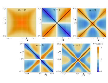
Figure 1: Color-scale plot of the Coulomb matrix elements $V_{J_{1},J_{2}}^{(m)}$ in the $J_{1}$-$J_{2}$ plane, normalized to their maximum value in the shown region, for Rashba parameter $\alpha=10$ and various $m$. Matrix elements taken along the solid lines are shown in Fig. 2.

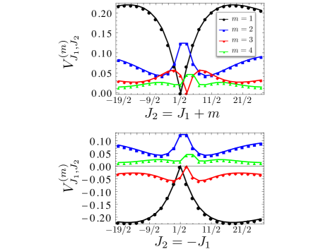
Figure 2: Coulomb matrix elements, in units of $\lambda\hbar\omega$, vs angular momentum $J_{2}$. The plots are for $\alpha=10$ and various $m$. The upper (lower) panel shows the case $J_{2}=J_{1}+m$ ($J_{2}=-J_{1}$), resp., cf. the solid lines in Fig. 1.

Numerical results for $\alpha=10$ and several $m$ are shown in Figs. 1 and 2. We draw the following conclusions:

• With increasing $|m|$, the absolute magnitude of the Coulomb matrix elements quickly decreases.

• Pronounced differences between even and odd $m$ are not yet visible for $\alpha=10$. Additional calculations for $\alpha=15$ and $\alpha=30$ (not shown here) confirm that the matrix elements for odd $m$ become more and more suppressed relative to the even-$m$ case. However, the ideal parity effect, where all odd-$m$ matrix elements vanish for $\alpha\to\infty$, is approached rather slowly.

• For $\alpha=10$, Figs. 1 and 2 show that the $V_{J_{1},J_{2}}^{(m)}$ carry a significant dependence on the indices $(J_{1},J_{2})$. This dependence ultimately disappears for $\alpha\to\infty$.

• For given value of $m$, the matrix element $V^{(m)}_{J_{1}J_{2}}$ has maximal absolute magnitude along the two lines $J_{2}=-J_{1}$ and $J_{2}=J_{1}+m$ in the $(J_{1},J_{2})$ plane. Noting that the single-particle eigenfunctions are localized near a ring of radius $k_{0}$ in momentum space, these two lines can be interpreted as BCS-like and exchange-type scattering processes, respectively, cf. the Appendix. The two lines of maximal absolute magnitude are orthogonal to each other, and cross at the point $(-m/2,m/2)$ in the ($J_{1},J_{2}$) plane. While for even $m$, this point is not a physically realized one (since $J_{1,2}$ must be half-integer), it is always the symmetry center.

• $V^{(m)}_{J_{1}J_{2}}$ is positive definite along the line $J_{2}=J_{1}+m$, for both even and odd $m$, while it is negative (positive) definite along the line $J_{2}=-J_{1}$ for odd (even) $m$.

• For even $m$, the interaction matrix elements are maximal at the four points where $(J_{1},J_{2})$ is either given by $\left(-\frac{m\pm 1}{2},\frac{m\pm 1}{2}\right)$ or by $\left(-\frac{m\pm 1}{2},\frac{m\mp 1}{2}\right)$. For odd $m$, the matrix elements vanish along the lines $J_{1}=-m/2$ and $J_{2}=m/2$, in accordance with the symmetry relation (31).

III Two interacting electrons for ultra-strong Rashba coupling

In this section, the $\alpha\to\infty$ model, $H_{\infty}$ [Eq. (28)], is studied for $N=2$ electrons. $H_{\infty}$ neglects all Coulomb matrix element contributions beyond Eq. (25), but includes the kinetic term $H_{0}$. We assume that the interaction strength is finite, but $\lambda\lesssim 1$ is needed to validate the single-band approximation.

III.1 Two-particle eigenstates

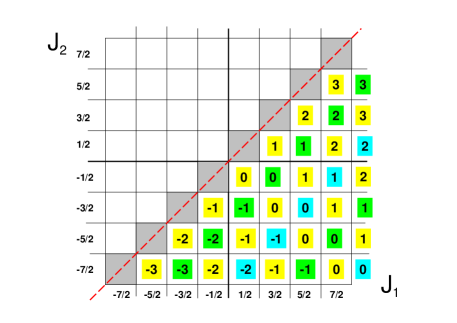
Figure 3: Schematic illustration of the invariant two-particle states $|M,\gamma\rangle$ (with integer $M$ and “family” index $\gamma=1,2,3$), see Eq. (32), in the $J_{1}$-$J_{2}$ plane. These states span the complete two-particle Hilbert space. Our ordering convention, $J_{1}>J_{2}$, implies that only states below the main diagonal (dashed red line) appear. Yellow cells correspond to $\gamma=1$, where the respective number indicates $M$. Green (blue) cells refer to $\gamma=2$ ($\gamma=3$). The interacting ground state has $\gamma=1$.

The two-particle Hilbert space is spanned by $c_{J_{1}}^{\dagger}c_{J_{2}}^{\dagger}|0\rangle$, where we set $J_{1}>J_{2}$ to avoid double counting and $|0\rangle$ is the $N=0$ state. This space is composed of decoupled subspaces, which are invariant under the action of $H_{\infty}$. The corresponding states, $|M,\gamma\rangle$, are labeled by the integer $M$ and a “family” index $\gamma=1,2,3$, see Fig. 3 for an illustration. With amplitudes $\beta_{J>0}$ subject to the normalization condition $\sum_{J>0}\left|\beta_{J}\right|^{2}=1$, and employing an auxiliary index $i_{\gamma}$ with values $i_{\gamma=1}=0$ and $i_{\gamma=2,3}=1$, those states are defined as

$$|M,\gamma\rangle=\sum_{J>0}\ \beta_{J}\ c_{J+M+i_{\gamma}}^{\dagger}c_{-J+M}^{\dagger}|0\rangle,$$ (32)

where for $\gamma=2$ ($\gamma=3$), only even (odd) $J+1/2$ are included in the summation.

Using the energies $E_{J}$ [Eq. (14)], some algebra shows that the action of $H_{\infty}$ on such a state yields

$$H_{\infty}|M,\gamma\rangle = \sum_{J,J^{\prime}>0}\Bigl{[}\left(E_{J+M+i_{\gamma}}+E_{-J+M}\right)\delta_{JJ^{\prime}}$$

$$+ 2\lambda\hbar\omega\left(S_{J-J^{\prime}}-\delta_{\gamma,1}S_{J+J^{\prime}}\right)\Bigr{]}$$

$$\times \beta_{J^{\prime}}\ c_{J+M+i_{\gamma}}^{\dagger}c_{-J+M}^{\dagger}|0\rangle,$$

with $S_{0}=0$ (see above). Equation (III.1) confirms that each family of states stays invariant under $H_{\infty}$. When looking for the ground-state energy, we note that an $M$-dependence can only originate from the $E_{J}\sim 1/\alpha^{2}$ terms. For $\alpha\to\infty$, all $|M,\gamma\rangle$ states with different $M$ but the same $\gamma$, therefore, have the same energy. As a consequence, the interacting ground state is highly degenerate for $\alpha\to\infty$. This degeneracy is only lifted by finite-$\alpha$ corrections resulting from the kinetic energy and from Coulomb matrix elements beyond $H_{\infty}$.

Importantly, since the energy-lowering contribution $-S_{J+J^{\prime}}$ is absent in Eq. (III.1) for $\gamma\neq 1$, the ground state must be in the $\gamma=1$ sector. The $\gamma=2,3$ states are separated by an energy gap $\sim\lambda\hbar\omega$, and we neglect these higher energy states from now on (and omit the $\gamma$ index). Since the magnetization operator $\hat{M}_{s}$ in Eq. (16) is conserved, the $|M\rangle$ states are also magnetization eigenstates. Indeed, one immediately finds that the corresponding eigenvalue is $M_{s}=2M\hbar$.

III.2 Distribution function

Figure 4: Distribution function, $n_{J}=\left|\beta_{J}\right|^{2}$, vs $J$ for the $N=2$ ground state of $H_{\infty}$. We here take $\lambda\alpha^{2}=10^{4}$, which leads to ${\cal E}_{\rm min}\simeq-0.0992725$. We stress that both $\beta_{J}$ (shown in the inset) as well as $n_{J}$ are independent of the total angular momentum, $M_{s}=2M\hbar$. Dotted lines serve as guides to the eye only.

For given total angular momentum, $M_{s}=2M\hbar$, we found in Sec. III.1 that the eigenstate of $H_{\infty}$ with lowest energy can be constructed from the Ansatz

$$|M\rangle=\sum_{J>0}\beta_{J}\ c_{J+M}^{\dagger}c_{-J+M}^{\dagger}|0\rangle,$$ (34)

with $\langle M^{\prime}|M\rangle=\delta_{MM^{\prime}}$. Clearly, the unmagnetized $M=0$ state in Eq. (34) describes a superposition of time-reversed states, and thus preserves the TRS of the Hamiltonian. However, TRS is violated by all other states, $|M\neq 0\rangle$.

Some algebra yields from Eq. (III.1) the matrix elements

$$\langle M^{\prime}|H_{\infty}|M\rangle=\left(\frac{M^{2}}{\alpha^{2}}+2\lambda{\cal E}\right)\delta_{MM^{\prime}}\hbar\omega,$$ (35)

with the dimensionless “energy”

$${\cal E}=\sum_{J,J^{\prime}>0}\left(\frac{J^{2}}{2\lambda\alpha^{2}}\delta_{JJ^{\prime}}+S_{J-J^{\prime}}-S_{J+J^{\prime}}\right)\beta_{J}\beta_{J^{\prime}}.$$ (36)

Since the matrix appearing in Eq. (36) is real symmetric, we can choose real-valued $\beta_{J}$. Moreover, since the matrix is independent of $M$, its lowest eigenvalue, ${\cal E}_{\rm min}$, is also $M$-independent and depends on the interaction strength and on the Rashba coupling only through the combination $\lambda\alpha^{2}$. The corresponding normalized eigenvector is easily obtained numerically and directly gives the $\beta_{J}$. Thereby we also obtain the normalized ground-state distribution function, $n_{J}=\left|\beta_{J}\right|^{2}$. Typical results for $\beta_{J}$ and $n_{J}$ are shown in Fig. 4. We find a rather broad distribution function $n_{J}$, very different from a Fermi function. To reasonable approximation, the numerical results can be fitted to a Gaussian decay, $n_{J}\sim e^{-(J/J^{*})^{2}}$, with $J^{*}\sim\sqrt{\alpha}$. Since $J^{*}\ll\alpha$, the relevant angular momentum states have $|J|\ll\alpha$, and the single-band approximation is self-consistently fulfilled. As shown in the inset of Fig. 4, the $\beta_{J}$ exhibit a pairwise oscillatory behavior, where $\beta_{J}<0$ for $J=1/2$ and $3/2$, but $\beta_{J}>0$ for $J=5/2$ and $7/2$, and so on.

III.3 Ground state magnetization

The above results indicate that for $\alpha\to\infty$ and given $M$, the lowest energy is

$$E^{(\infty)}_{M}=\left(\frac{M^{2}}{\alpha^{2}}+2\lambda{\cal E}_{\rm min}\right)\hbar\omega.$$ (37)

While this suggests that the ground state has $M=0$, the $M^{2}/\alpha^{2}$ term (due to $H_{0}$) is in fact subleading to Coulomb corrections beyond $H_{\infty}$, which approximately scale $\sim 1/\alpha$, see Eq. (58). We therefore have to take these Coulomb matrix elements into account when determining the ground state. To that end, using the symmetry relation (29), and exploiting that $\hat{M}_{s}$ is conserved, we note that $H_{I}$ [Eq. (18)] has the matrix elements

$$\langle M^{\prime}|H_{I}|M\rangle=2\delta_{MM^{\prime}}\sum_{J,J^{\prime}>0}\beta_{J}\beta_{J^{\prime}}$$ (38)

$$\times\left(V^{(J-J^{\prime})}_{-J+M,J+M}-V^{(J+J^{\prime})}_{-J+M,J+M}\right).$$

Therefore, the energies $E_{M}^{(\infty)}$ in Eq. (37) will be independently shifted by this perturbation, and the $(J_{1},J_{2})$-dependence of the Coulomb matrix elements becomes important, see Sec. II.4. In particular, terms with odd angular momentum exchange $m$ will contribute. Treating the Coulomb corrections in perturbation theory, the lowest energy for fixed $M$ is

$$E_{M}=E_{-M}=E^{(\infty)}_{M}+\langle M|H_{I}|M\rangle-2\lambda{\cal E}_{\rm min}\hbar\omega,$$ (39)

where $E_{M}=E_{-M}$ follows from the symmetry relations in Sec. II.4. Comparing $E_{M}$ to the respective $M=0$ value, $\delta E_{M}=E_{M}-E_{M=0}$, we finally obtain

$$\delta E_{M}=\frac{M^{2}}{\alpha^{2}}\hbar\omega+\langle M|H_{I}|M\rangle-\langle M=0|H_{I}|M=0\rangle,$$ (40)

with $\langle M|H_{I}|M\rangle$ in Eq. (38).

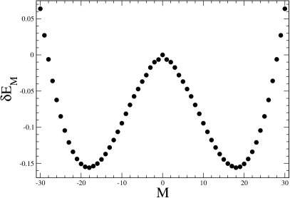
Figure 5: Lowest two-particle energy for fixed $M$ relative to the $M=0$ state, $\delta E_{M}$ [Eq. (40)], vs $M$. We here consider $\alpha=30$ and $\lambda=1$, where $\delta E_{M}$ is given in units of $\hbar\omega$.

The numerical result for $\delta E_{M}$ is shown in Fig. 5, where we take $\alpha=30$ and $\lambda=1$ as concrete example. Interestingly, the unmagnetized $M=0$ state represents a local energy maximum. This can be rationalized by noting that the $\beta_{J}$ have pairwise alternating sign, see Fig. 4. For small but non-zero $|M|$, Eq. (38) is thus dominated by the $J=J^{\prime}$ contribution due to $V^{(J-J^{\prime})}_{-J+M,J+M}$, resulting in the estimate

$$\delta E_{M}\approx 2\sum_{J>0}n_{J}\left(V^{(0)}_{-J+M,J+M}-V^{(0)}_{-J,J}\right)<0.$$ (41)

The inequality here follows by noting that Coulomb matrix elements with $m=0$ are always positive and have a maximum for $|J_{2}|=|J_{1}|$, cf. Sec. II.4. For large $|M|$, however, the $M^{2}$ contribution in Eq. (40) becomes crucial. As a consequence, we arrive at a symmetric double-well behavior for $\delta E_{M}$, with two minima at $M=\pm M_{0}$. This simple argument is consistent with our numerical results based on Eq. (39), see Fig. 5.

Since we typically find $M_{0}\gg 1$, see Fig. 5, this effect must come from the orbital angular momentum. The value of $M_{0}=M_{0}(\alpha,\lambda)$ can be estimated analytically as follows. Evaluating $\delta E_{M}$ from Eq. (40), employing the approximation in Eq. (41) and the expression for the matrix elements in Eq. (58), we find

$$\frac{\delta E_{M}}{\hbar\omega}\simeq\frac{M^{2}}{\alpha^{2}}-\frac{2\lambda}{\pi\alpha}\int_{0}^{\pi/2}d\varphi\frac{\sin\varphi}{\cos^{2}\varphi}\sin^{2}(2M\varphi).$$ (42)

The minimum of $\delta E_{M}$ with $M=+M_{0}$ then follows from the equation

$$M_{0}=\frac{2\lambda\alpha}{\pi}\int_{0}^{\pi/2}d\varphi\frac{\varphi\sin\varphi}{\cos^{2}\varphi}\sin(4M_{0}\varphi).$$ (43)

Assuming $M_{0}\gg 1$, the main contribution to the integral comes from $\varphi\lesssim 1/M_{0}$, and performing the subsequent integration implies $M_{0}\approx(\lambda\alpha)^{1/4}$. Clearly, this suggests that $M_{0}$ can be very large even for weak interactions.

The ground state of the $N=2$ dot,

$$|\Phi\rangle=\sum_{\pm}c_{\pm}|\pm M_{0}\rangle,\quad\sum_{\pm}|c_{\pm}|^{2}=1,$$ (44)

is spanned by the two degenerate states $|\pm M_{0}\rangle$, with magnetization $M_{s}=\pm 2M_{0}\hbar$, respectively. Unless $c_{+}c_{-}=0$, we note that $|\Phi\rangle$ is not an eigenstate of the conserved operator $\hat{M}_{s}$. However, the magnetization expectation value, $\langle\Phi|\hat{M}_{s}|\Phi\rangle=2(|c_{+}|^{2}-|c_{-}|^{2})M_{0}\hbar$, is finite except when $|c_{+}|=|c_{-}|$. This suggests that by application of a weak magnetic field perpendicular to the 2D plane, the magnetization can be locked to one of the two minima, say, $M_{s}=+2M_{0}\hbar$. Adiabatically switching off the magnetic field, we then expect $|\Phi\rangle=|M_{0}\rangle$, since there is an energy barrier to the $|-M_{0}\rangle$ state. Since the barrier is not infinite, we cannot exclude that quantum-mechanical tunneling effects will ultimately establish an unmagnetized ground state with $|c_{+}|=|c_{-}|$, in particular when taking into account violations of the perfect rotational symmetry of the dot assumed in our model. For instance, such imperfections correspond to an eccentricity of the confinement potential or the presence of nearby impurities. As long as such imperfections represent a weak perturbation, however, the associated tunneling timescales connecting the two degenerate states $|\pm M_{0}\rangle$ are expected to be very long. We shall discuss this issue in some detail in Sec. V.

For practical purposes, assuming that quantum tunneling is not relevant on the timescales of experimental interest, adiabatically switching off the magnetic field then effectively results in the ground state $|\Phi\rangle=|M_{0}\rangle$. This state carries a large magnetization, $M_{s}=2M_{0}\hbar$, and thus also a circulating charge current. Such a state appears to spontaneously break the TRS of the Hamiltonian, and is interpreted here as a “molecular” orbital ferromagnet.

The above discussion pertains to the idealized $T=0$ case. In practice, the zero-temperature limit also governs the physics at temperatures well below the above energy barrier, $k_{B}T\ll|\delta E_{M_{0}}|$. However, at higher temperatures, thermally induced transitions between both minima happen on short timescales, and the overall magnetization of the dot vanishes. Nonetheless, $\hat{M}_{s}^{2}$ still has a finite expectation value.

III.4 Spin and charge density

Before proceeding with a discussion of numerical results for $N>2$, let us briefly address the spin and charge density for $\alpha\to\infty$. We assume that the $N=2$ system is in a definite ground state, say $|M_{0}\rangle$.

The total spin density at position $\bm{r}=r(\cos\theta,\sin\theta)$ follows as

$$\bm{S}(r,\theta)=\sum_{J>0}n_{J}\left[\bm{s}_{J+M_{0}}(r,\theta)+\bm{s}_{-J+M_{0}}(r,\theta)\right],$$ (45)

where $\bm{s}_{J}=(s^{x}_{J},s^{y}_{J},s^{z}_{J})$ is the spin density for the single-particle state $\tilde{\psi}_{J}(r,\theta)$. Using Eq. (24), we obtain, e.g.,

$$s^{x}_{J}(r,\theta)\simeq\frac{\hbar}{2}\frac{e^{-r^{2}/l_{T}^{2}}}{\pi^{3/2}l_{T}r}\cos(\theta)\sin(2k_{0}r-\pi J).$$ (46)

As a consequence, the two contributions in Eq. (45) precisely cancel each other, and $S^{x}=0$. By the same argument, we also find that the $y$- and $z$-components of the spin density vanish. In the limit $\alpha\to\infty$, the spin density $\bm{S}$ is therefore identically zero. In practice, finite contributions may come from subleading ($\sim 1/\alpha$) terms, but these are small for $\alpha\gg 1$.

We now turn to the charge density, $\rho_{c}(r)$, which is always radially symmetric. For $\alpha\to\infty$, all single-particle states, $\tilde{\psi}_{J}$ in Eq. (24), lead to the same probability density in space, and we therefore conclude that $\rho_{c}(r)$ must be independent of Coulomb interactions. For $\lambda\lesssim 1$ and arbitrary particle number $N$, we thus obtain

$$\rho_{c}(r)=\frac{eN}{\pi^{3/2}l_{T}r}e^{-r^{2}/l_{T}^{2}},$$ (47)

which satisfies the expected normalization, $2\pi\int_{0}^{\infty}drr\rho_{c}(r)=eN$. We mention in passing that the “edge” state property of the single-particle states, i.e., states with larger $|J|$ live further away from the dot center, can be seen from the finite-$\alpha$ wavefunctions in Eq. (13) li1 , but not anymore from their asymptotic $\alpha\to\infty$ form in Eq. (24). The $\lambda$-independence of $\rho_{c}(r)$ at large $\alpha$ is in marked contrast to the case of weak spin-orbit coupling, where $\rho_{c}$ contains information about interactions and can be used to detect Wigner molecule formation egger ; weissegger . Instead, the charge density in Eq. (47) is featureless for arbitrary $N$, pointing once again to the absence of the Wigner molecule for $\alpha\gg 1$ and $\lambda\lesssim 1$. Finally, we note that by computing the pair distribution function giul , we also find no trace of Wigner molecule formation in this limit.

IV Exact diagonalization and Hartree-Fock calculations

We now discuss numerical results for the ground-state energy and magnetization for $N\leq 10$ electrons in the dot. These results were obtained by means of the standard exact diagonalization technique and by Hartree-Fock (HF) theory from $H=H_{0}+H_{I}$, with $H_{0}$ in Eq. (14), $H_{I}$ in Eq. (18), and the Coulomb matrix elements (22), see Sec. II. This implies that the following results are not restricted to the $\alpha\to\infty$ limit considered in Sec. III. However, we are limited to rather weak interactions, $\lambda\lesssim 1$, and moderate particle numbers, $N<\alpha$, because of our single-band approximation. We first describe our exact diagonalization results and then turn to HF theory.

IV.1 Exact diagonalization

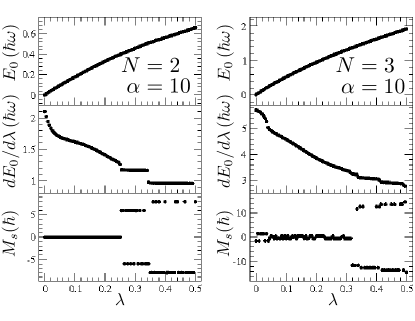
Figure 6: Exact diagonalization results for the ground-state energy, $E_{0}$, and the magnetization, $M_{s}$, vs interaction parameter $\lambda$, for $\alpha=10$ and $N=2$ (left) and $N=3$ (right). The top row shows $E_{0}(\lambda)$, where singular structures are visible in the derivative, $dE_{0}/d\lambda$, as depicted in the center panel. The bottom panel shows the magnetization, $M_{s}$, where $M_{s}\neq 0$ for $\lambda>\lambda_{c}$. (For $N=3$, a finite but very small value for $M_{s}$ numerically appears already for $\lambda_{c}<0.31$.)

Using the Rashba parameter $\alpha=10$, exact diagonalization results for $N=2$ and $N=3$ electrons in the dot are shown in Fig. 6. While $E_{0}(\lambda)$ at first sight seems rather featureless (top panel), there are non-analytic features that become visible when plotting the first derivative (center panel). Let us discuss this point in detail for $N=2$, see the left side of Fig. 6. The first non-analytic feature occurs at $\lambda_{c}\approx 0.25$, where the second derivative diverges, $d^{2}E_{0}/d\lambda^{2}\to-\infty$, as the interaction parameter $\lambda$ approaches the critical value $\lambda_{c}$ from below. In close analogy to the results obtained from $H_{\infty}$ in Sec. III, the ground state for $\lambda>\lambda_{c}$ has the magnetization $M_{s}=\pm 2M_{0}\hbar$, where $M_{0}$ is integer and the ground state is degenerate with respect to both signs. In the exact diagonalization, the “initial conditions” selecting the eventually realized state ($M_{s}=+2M_{0}\hbar$ or $M_{s}=-2M_{0}\hbar$) correspond to unavoidable numerical rounding errors. In contrast to the $\alpha\to\infty$ limit, however, the interaction parameter $\lambda$ must now exceed a critical value, $\lambda_{c}$, to allow for the orbital ferromagnet. For $\lambda<\lambda_{c}$, the $M=0$ state is the ground state, which is adiabatically connected to the noninteracting ground state. Since energy levels of states with different conserved total angular momentum $M_{s}$ can cross each other, the critical value $\lambda_{c}$ marks a quantum phase transition. However, once disorder or eccentricity of the quantum dot are present, angular momentum conservation breaks down and the transition will correspond to a smooth crossover phenomenon. The observed large value of the magnetization, $|M_{s}|=6\hbar$ for $\lambda>\lambda_{c}$, see Fig. 6, again rules out a purely spin-based explanation. In fact, additional jumps to even higher $|M_{s}|$ are observed for larger $\lambda$ in Fig. 6.

Similar features are also observed for $N=3$, where exact diagonalization results are shown on the right side of Fig. 6. Again, the first derivative of $E_{0}(\lambda)$ displays non-analytic behavior. For small $\lambda$, the state stays close to a doubly degenerate Fermi sea, see Sec. II.1. For $\lambda>\lambda_{c}\approx 0.31$, however, a large magnetization emerges, $|M_{s}|=11.5\hbar$.

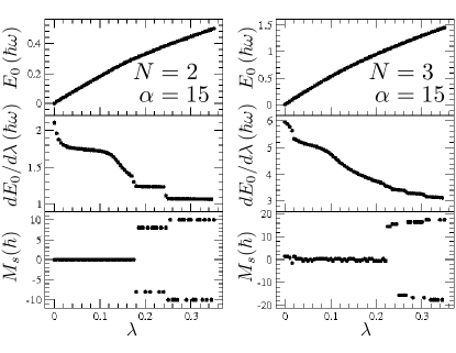
Figure 7: Same as Fig. 6 but for $\alpha=15$.

The results of Sec. III show that the critical interaction strength $\lambda_{c}$ vanishes for $\alpha\to\infty$. We therefore expect $\lambda_{c}$ to decrease with increasing $\alpha$. To study this point, exact diagonalization results for $\alpha=15$ are shown in Fig. 7. All qualitative features observed for $\alpha=10$ are recovered, and the critical value $\lambda_{c}$ is indeed found to decrease: For $N=2$, we now find $\lambda_{c}\approx 0.17$ (instead of $\lambda_{c}\approx 0.25$ for $\alpha=10$), while for $N=3$, we obtain $\lambda_{c}\approx 0.22$ (instead of $\lambda_{c}\approx 0.31$). This confirms that with increasing spin-orbit coupling strength, the orbital ferromagnetic state is reached already for weaker interactions.

IV.2 Hartree-Fock calculations

Finally, let us turn to numerical results for larger $N$, where exact diagonalization becomes computationally too expensive. We have carried out an unrestricted Hartree-Fock analysis following the textbook formulation giul , in order to find the energy and the total angular momentum of the $N$-electron ground state. We note that HF calculations are known to provide a reasonable description for $\alpha=0$ landman ; reusch1 ; reusch2 . We find that a diagonal HF density matrix is sufficient, with variational parameters $n_{J}=\langle c_{J}^{\dagger}c_{J}\rangle$ for half-integer $J$ subject to the normalization condition $\sum_{J}n_{J}=N$. Up to a constant, the resulting HF Hamiltonian is given by

$$H_{\rm HF}=\sum_{J}\left(E_{J}+2\sum_{J^{\prime}}\left[V_{J,J^{\prime}}^{(0)}-V_{J,J^{\prime}}^{(J^{\prime}-J)}\right]n_{J^{\prime}}\right)c_{J}^{\dagger}c_{J}.$$ (48)

The self-consistent HF ground state is numerically found by iteration, starting from randomly chosen initial distributions. The converged $\{n_{J}\}$ distribution yields the magnetization, $M_{s}$, and the ground-state energy. For $\lambda$ approaching the (HF value of the) critical interaction parameter, $\lambda_{c}(\alpha,N)$, the energy shows similar non-analytic features as found from exact diagonalization, see Sec. IV.1. For $\lambda>\lambda_{c}$, a large ground-state magnetization is observed, again corresponding to orbital ferromagnetism.

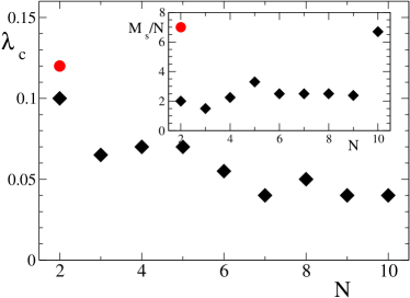
Figure 8: Hartree-Fock results (black diamonds) for the critical interaction strength $\lambda_{c}$ vs particle number $N$ for $\alpha=30$ (main panel). The red circle shows the corresponding exact diagonalization result for $N=2$. Inset: Magnetization $M_{s}$ (in units of $\hbar N$) found for $\lambda\gtrsim\lambda_{c}$, vs particle number $N$.

Our HF results for $\lambda_{c}$ and $M_{s}$ are shown in Fig. 8. We consider the Rashba spin-orbit coupling $\alpha=30$, and up to $N=10$ electrons in the dot. Unfortunately, we cannot address larger $N$, for otherwise our single-band approximation is not justified anymore. For $N=2$, the corresponding exact diagonalization values are also given. The HF value for $\lambda_{c}$ is only slightly smaller than the exact one, which suggests that HF theory is at least qualitatively useful. That the HF prediction is below the exact one for $N=2$ can be rationalized by noting that HF theory generally tends to favor ordered phases such as orbital ferromagnetism, resulting in a smaller value for $\lambda_{c}$. The magnetization for $\lambda>\lambda_{c}$, however, is a more difficult quantity to predict due to the shallow minima of the free energy curves in Fig. 5. Indeed, the inset of Fig. 8 shows that the HF value of the magnetization (which appears to scale as $M_{s}\sim N$) is significantly smaller than the exact one. With increasing $N$, the HF predictions for $\lambda_{c}$ indicate that the transition to the orbital ferromagnet persists. Moreover, this transition can even be reached at weaker interactions.

V Discussion

In this work, we have studied the interacting $N$-electron problem for a parabolic 2D quantum dot (with $N\leq 10$) in the limit of strong Rashba spin-orbit coupling, $\alpha\gg 1$. This regime is characterized by an almost flat single-particle spectrum, where we find that already weak-to-intermediate Coulomb interactions (our single-band approximation permits us to study the regime $\lambda\lesssim 1$ only) are sufficient to induce molecular orbital ferromagnetism. This state is observed for $\lambda>\lambda_{c}(\alpha,N)$, where our $N=2$ solution in Sec. II shows that the critical strength $\lambda_{c}\to 0$ for $\alpha\to\infty$. For finite (but large) $\alpha$, however, $\lambda_{c}$ will be finite. The orbital ferromagnet has a giant total angular momentum, accompanied by a circulating charge current.

Coming back to our discussion in Sec. III.3, we now address issues concerning the experimental observation of the predicted orbital ferromagnetism for a single quantum dot. The transition to this state could be induced in practice by varying the electrostatic confinement potential and/or the gate-controlled Rashba spin-orbit coupling in order to reach the regime defined by $\alpha\gg 1$ and $\lambda>\lambda_{c}$. By allowing for an eccentricity of the dot confinement potential, which also can be achieved with appropriate gate voltages, quantum tunneling processes connecting the free energy minima with opposite magnetization, $M_{s}=\pm M_{\rm min}$, are expected to become relevant, see Sec. III.3. The corresponding timescale for such processes can be estimated as follows. We first note that the free energy barrier between both minima, $B\hbar\omega$, corresponds to a number $B\approx 0.1\ldots 0.15$, see Fig. 5. We next employ a paradigmatic effective low-energy model to include the effects of imperfections breaking the ideal rotational symmetry,

$$H_{\rm eff}=\left[\frac{\epsilon}{2}\phi^{2}+B\frac{(M_{s}^{2}-M_{\rm min}^{2})^{2}}{M_{\rm min}^{4}}\right]\hbar\omega.$$ (49)

The first term describes the dot eccentricity, with a small dimensionless parameter $\epsilon$, where the polar angle $\phi$ is conjugate to the magnetization $M_{s}$. The second term approximates the double-well potential in Fig. 5. The two lowest eigenenergies for $H_{\rm eff}$ are known exactly alexal . From the result, we find the level splitting

$$\delta E=\sqrt{\frac{2}{\pi}}64B\hbar\omega\exp\left(-\frac{4\sqrt{2B}}{3\sqrt{\epsilon}}M_{\rm min}\right).$$ (50)

The resulting timescale for tunneling processes, $\tau$, is thereby estimated as

$$\omega\tau=\frac{\hbar\omega}{\delta E}\approx 0.2e^{5.96M_{\rm min}}.$$ (51)

where, for simplicity, we have put $B=0.1$ and $\epsilon=0.01$. For the value $M_{\rm min}\approx 18$ observed in Fig. 5, we get the estimate $\omega\tau\approx 10^{45}$. This astronomically long tunneling time strongly suggests that on experimentally accessible timescales, the orbital ferromagnet described in this paper will be indistinguishable from a true equilibrium state.

It is also useful to contrast the behavior reported here to the well-known persistent currents in normal-metal quantum rings buttiker ; gogolinring ; tapashring ; hauslerring ; tanring , where a circulating equilibrium electric current flows and can be experimentally detected, see Ref. pcexp and references therein. First, a persistent current flows already in noninteracting quantum rings but requires a nonzero flux threading the ring, while orbital ferromagnetism in a 2D dot is generated by the interplay of Coulomb interactions and strong spin-orbit coupling. Second, the total angular momentum (magnetization) predicted here for a 2D Rashba dot can be very large. Therefore, the circulating currents in our case should exceed the persistent currents observed in quantum rings by far. Despite of these differences, the persistent current analogy also suggests ways to observe our predictions experimentally. Another possibility is to study the response to a weak magnetic field applied perpendicular to the 2D plane. The low-field susceptibility is then expected to be singular, just as in an ordinary ferromagnet. At elevated temperatures approaching the free energy barrier height discussed above, the orbital magnetization in our system will be thermally suppressed and ultimately disappear. The relevant temperature scale for this crossover is $T_{c}\approx B\hbar\omega/k_{B}$. For typical quantum dots kouwenhoven , $T_{c}\approx 1$ to 10 K.

To conclude, we hope that our prediction of orbital ferromagnetism in Rashba dots will stimulate further theoretical and experimental work. For instance, it remains an open question to address the transition from the orbital ferromagnet to a Wigner molecule with increasing interaction strength for large Rashba coupling. In order to achieve this description, one needs to go beyond the single-band approximation employed in this work.

Appendix A On ultra-strong Rashba couplings

In this Appendix, we address an alternative calculation of the interaction matrix elements $V_{J_{1},J_{2}}^{(m)}$ for $\alpha\to\infty$. Instead of taking this limit as $k_{0}\to\infty$ with finite $l_{T}$, see Sec. II.3, we here formally assume a fixed spin-orbit momentum $k_{0}$ but large $l_{T}$. The $\alpha\to\infty$ limit taken in this manner is subtle since (i) the resulting expressions require infrared regularization with $l_{T}$ setting the effective system size, and (ii) the single-band approximation requires a finite confinement frequency in order to be justified. However, it is also beneficial since one can proceed directly in momentum space and thereby obtain an intuitive understanding of the parity effect.

We start by noting that the states (8) describe a Gaussian distribution of the probability density in momentum space around $k=k_{0}$, where $1/l_{T}$ sets the amplitude of zero-point fluctuations of $k$ around $k_{0}$. For $l_{T}\to\infty$, this density becomes $\left|\psi_{J}({\bf k})\right|^{2}\simeq(2\pi/k_{0})\ \delta(k-k_{0})$. The states (8) thus have the limiting behavior

$$\psi_{J}({\bf k})\simeq\sqrt{\frac{2\pi^{3/2}}{k_{0}l_{T}}}e^{i(J-1/2)\phi}\delta(k-k_{0})\left(\begin{array}[]{c}1\\ -ie^{i\phi}\end{array}\right),$$ (52)

describing localization on a ring in momentum space. The interaction Hamiltonian is

$$H_{I}=\frac{1}{2}\int\frac{d^{2}{\bf q}}{(2\pi)^{2}}\,\frac{2\pi e^{2}}{\varepsilon_{0}q}:\rho(-{\bf q})\rho({\bf q}):,$$ (53)

where $::$ denotes normal ordering and

$$\rho({\bf q})=\int\frac{d^{2}{\bf k}}{(2\pi)^{2}}\,\Psi_{{\bf k}+{\bf q}}^{\dagger}\Psi_{{\bf k}},\quad\Psi_{\bf k}=\sum_{J}\psi_{J}({\bf k})c_{J}.$$ (54)

Writing

$${\bf k}=k\left(\begin{array}[]{c}\cos\phi\\ \sin\phi\end{array}\right),\quad{\bf q}=q\left(\begin{array}[]{c}\cos\vartheta\\ \sin\vartheta\end{array}\right),\quad{\bf k}^{\prime}={\bf k}+{\bf q},$$ (55)

it is now crucial to take into account the constraints $k=k^{\prime}=k_{0}$ coming from the $\delta$-functions in $\psi_{J}({\bf k})$. In effect, all momenta for incoming, ${\bf k}_{1,2}$, and outgoing, ${\bf k}^{\prime}_{1,2}$, electrons must be located on a ring of radius $k_{0}$ in momentum space. This severe phase-space restriction is only met by two types of interaction processes as explained next.

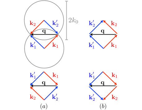
Figure 9: Coulomb two-particle scattering processes, ${\bf k}_{1,2}\to{\bf k}_{1,2}^{\prime}={\bf k}_{1,2}\pm{\bf q}$, for given exchanged momentum, ${\bf q}$, in the $\alpha\to\infty$ limit, where all particle momenta are constrained to a ring of radius $k_{0}$. For ${\bf q}\neq 0$, only four interaction processes are possible, which can be grouped into two classes: (a) BCS-like scattering of a pair of opposite-momentum states, ${\bf k}_{1}=-{\bf k}_{2}$, into another pair with ${\bf k}_{1}^{\prime}=-{\bf k}_{2}^{\prime}$, and (b) exchange-type scattering processes, $({\bf k}_{1},{\bf k}_{2})\to({\bf k}_{1}^{\prime}={\bf k}_{2},{\bf k}_{2}^{\prime}={\bf k}_{1})$.

Shifting the integration variable $\phi\to\phi+\vartheta$, some algebra yields (integer $m$) mathfoot

$$V_{J_{1},J_{2}}^{(m)}=\frac{e^{2}}{4\varepsilon_{0}l_{T}^{2}}\int_{0}^{2k_{0}}dq\int_{0}^{2\pi}\frac{d\phi_{1}d\phi_{2}}{2\pi}$$ (56)

$$\times~{}~{}\delta(k_{1}^{\prime}-k_{0})\ \delta(k_{2}^{\prime}-k_{0})e^{im(\phi_{2}-\phi_{1})}\sum_{\sigma_{1},\sigma_{2}=\pm}$$

$$\times~{}~{}\left(1+\frac{q}{k_{0}}e^{i\phi_{1}}\right)^{J_{1}+m+\sigma_{1}/2}\left(1-\frac{q}{k_{0}}e^{i\phi_{2}}\right)^{J_{2}-m+\sigma_{2}/2},$$

where the $\delta$-function implies the constraint

$$k_{1}^{\prime}(\phi_{1})=\sqrt{k_{0}^{2}+q^{2}+2k_{0}q\cos\phi_{1}}=k_{0},$$ (57)

and similarly for $k_{2}^{\prime}$. This leads to the condition $\cos\phi_{1}=-\cos\phi_{2}=-q/2k_{0}$, which is met by two types of scattering processes only, namely (a) for $\phi_{2}=\pi+\phi_{1}$ (BCS-like pairing), and (b) for $\phi_{2}=\pi-\phi_{1}$ (exchange-type process), see Fig. 9. Such spin-orbit-induced constraints on interaction processes were also recently pointed out in Ref. scring . Parametrizing $q=2k_{0}\cos\varphi$ in Eq. (56), we obtain

$$V_{J_{1},J_{2}}^{(m)}=(-1)^{J_{1}+J_{2}+m-1}\frac{e^{2}}{2\pi\varepsilon_{0}k_{0}l^{2}_{T}}\int_{0}^{\pi/2}d\varphi$$ (58)

$$\times~{}~{}\sin\varphi\frac{-\cos[2(J_{1}+J_{2})\varphi]+\cos[2(J_{1}-J_{2}+m)\varphi]}{\cos^{2}\varphi},$$

where the first (second) term in the numerator results from BCS-like (exchange-type) processes. Importantly, the above integral is infrared divergent for $q=2k_{0}\cos\varphi\to 0$. To regularize this singularity, we employ $l_{T}$ as effective system size and require $ql_{T}>1$. After some algebra, we find the ($J_{1},J_{2}$)-independent result $V_{J_{1},J_{2}}^{(m)}\simeq\lambda\hbar\omega\delta_{m,\textrm{even}}$, which recovers the parity effect in Sec. II.3, including the $(J_{1},J_{2})$-independence of the matrix elements. In contrast to Eq. (25), however, the even-$m$ Coulomb matrix elements found here are also independent of $m$. This indicates that the limits $k_{0}\to\infty$ and $l_{T}\to\infty$ do not commute.

References

- (1) Yu.V. Nazarov and Ya.M. Blanter, Quantum Transport: Introduction to Nanoscience (Cambridge University Press, Cambrige, UK, 2009).
- (2) L.P. Kouwenhoven, D.G. Austing, and S. Tarucha, Few-electron quantum dots, Rep. Prog. Phys. 64, 701 (2001).
- (3) S.M. Reimann and M. Manninen, Electronic structure of quantum dots, Rev. Mod. Phys. 74, 1283 (2002).
- (4) C. Yannouleas and U. Landman, Symmetry breaking and quantum correlations in finite systems: Studies of quantum dots and ultracold Bose gases and related nuclear and chemical methods, Rep. Prog. Phys. 70, 2067 (2007).
- (5) R. Egger, W. Häusler, C.H. Mak, and H. Grabert, Crossover from Fermi Liquid to Wigner Molecule Behavior in Quantum Dots, Phys. Rev. Lett. 82, 3320 (1999).
- (6) K. Jauregui, W. Häusler, and B. Kramer, Wigner Molecules in Nanostructures, EPL 24, 581 (1993).
- (7) F. Bolton and U. Rössler, Classical model of a Wigner crystal in a quantum dot, Superlatt. Microstruct. 13, 139 (1993).
- (8) V.M. Bedanov and F.M. Peeters, Ordering and phase transitions of charged particles in a classical finite two-dimensional system, Phys. Rev. B 49, 2667 (1994).
- (9) R. Winkler, Spin-orbit coupling effects in two-dimensional electron and hole systems (Springer Verlag Berlin, 2003).
- (10) O. Voskoboynikov, C.P. Lee, and O. Tretyak, Spin-orbit splitting in semiconductor quantum dots with a parabolic confinement potential, Phys. Rev. B 63, 165306 (2001).
- (11) P. Pietiläinen and T. Chakraborty, Energy levels and magneto-optical transitions in parabolic quantum dots with spin-orbit coupling, Phys. Rev. B 73, 155315 (2006).
- (12) M. Governale, Quantum Dots with Rashba Spin-Orbit Coupling, Phys. Rev. Lett. 89, 206802 (2002).
- (13) A. Emperador, E. Lipparini, and F. Pederiva, Role of spin-orbit interaction in the chemical potential of quantum dots in a magnetic field, Phys. Rev. B 70, 125302 (2004).
- (14) S. Weiss and R. Egger, Path-integral Monte Carlo simulations for interacting few-electron quantum dots with spin-orbit coupling, Phys. Rev. B 72, 245301 (2005).
- (15) A. Ambrosetti, F. Pederiva, and E. Lipparini, Quantum Monte Carlo study of circular quantum dots in presence of Rashba interaction, Phys. Rev. B 83, 155301 (2011).
- (16) C.F. Destefani, S.E. Ulloa, and G.E. Marques, Spin-orbit coupling and intrinsic spin mixing in quantum dots, Phys. Rev. B 69, 125302 (2004).
- (17) C.F. Destefani, S.E. Ulloa, and G.E. Marques, Spin-orbit and electronic interactions in narrow-gap quantum dots, Phys. Rev. B 70, 205315 (2004).
- (18) T. Chakraborty and P. Pietiläinen, Electron correlations in a quantum dot with Bychkov-Rashba coupling, Phys. Rev. B 71, 113305 (2005).
- (19) A. Cavalli, F. Malet, J.C. Cremon, and S.M. Reimann, Spin-orbit-enhanced Wigner localization in quantum dots, Phys. Rev. B 84, 235117 (2011).
- (20) E. Berg, M.S. Rudner, and S.A. Kivelson, Electronic liquid crystalline phases in a spin-orbit coupled two-dimensional electron gas, Phys. Rev. B 85, 035116 (2012).
- (21) P.G. Silvestrov and O. Entin-Wohlmann, Wigner crystal of a two-dimensional electron gas with a strong spin-orbit interaction, Phys. Rev. B 89, 155103 (2014).
- (22) M. Kohda, T. Bergsten, and J. Nitta, Manipulating Spin-Orbit Interaction in Semiconductors, J. Phys. Soc. Jpn. 77, 031008 (2008).
- (23) L. Meier, G. Salis, I. Shorubalko, E. Gini, S. Schön, and K. Ensslin, Measurement of Rashba and Dresselhaus spin-orbit magnetic fields, Nat. Phys. 3, 650 (2007).
- (24) C.R. Ast, J. Henk, A. Ernst, L. Moreschini, M.C. Falub, D. Pacilé, P. Bruno, K. Kern, and M. Grioni, Giant Spin Splitting through Surface Alloying, Phys. Rev. Lett. 98, 186807 (2007).
- (25) C.R. Ast, D. Pacilé, L. Moreschini, M.C. Falub, M. Papagno, K. Kern, and M. Grioni, Spin-orbit split two-dimensional electron gas with tunable Rashba and Fermi energy, Phys. Rev. B 77, 081407(R) (2008).
- (26) I. Gierz, T. Suzuki, E. Frantzeskakis, S. Pons, S. Ostanin, A. Ernst, J. Henk, M. Grioni, K. Kern, and C.R. Ast, Silicon Surface with Giant Spin Splitting, Phys. Rev. Lett. 103, 046803 (2009).
- (27) K. Yaji, Y. Ohtsubo, S. Hatta, H. Okuyama, K. Miyamoto, T. Okuda, A. Kimura, H. Namatame, M. Taniguchi, and T. Aruga, Large Rashba spin splitting of a metallic surface-state band on a semiconductor surface, Nat. Commun. 1, 17 (2010).
- (28) Y. Kanai, R.S. Deacon, S. Takahashi, A. Oiwa, K. Yoshida, K. Shibata, K. Hirakawa, Y. Tokura, and S. Tarucha, Electrically tuned spin-orbit interaction in an InAs self-assembled quantum dot, Nat. Nanotech. 6, 511 (2011).
- (29) H. Murakawa, M.S. Bahramy, M. Tokunaga, Y. Kohama, C. Bell, Y. Kaneko, N. Nagaosa, H.Y. Hwang, and Y. Tokura, Detection of Berry’s Phase in a Bulk Rashba Semiconductor, Science 342, 1490 (2013).
- (30) M.Z. Hasan and C.L. Kane, Colloquium: Topological insulators, Rev. Mod. Phys. 82, 3045 (2010).
- (31) X.L. Qi and S.C. Zhang, Topological insulators and superconductors, Rev. Mod. Phys. 83, 1057 (2011).
- (32) Y. Li, X. Zhou, and C. Wu, Two- and three-dimensional topological insulators with isotropic and parity-breaking Landau levels, Phys. Rev. B 85, 125122 (2012).
- (33) Y. Li, S.C. Zhang, and C. Wu, Topological Insulators with SU(2) Landau Levels, Phys. Rev. Lett. 111, 186803 (2013).
- (34) E. Rashba, Quantum nanostructures in strongly spin-orbit coupled two-dimensional systems, Phys. Rev. B 86, 125319 (2012).
- (35) S.K. Ghosh, J.P. Vyasanakere, and V.B. Shenoy, Trapped fermions in a synthetic non-Abelian gauge field, Phys. Rev. A 84, 053629 (2011).
- (36) C. Echeverría-Arrondo and E.Ya. Sherman, Position and spin control by dynamical ultrastrong spin-orbit coupling, Phys. Rev. B 88, 155328 (2013).
- (37) W. Witczak-Krempa, G. Chen, Y.B. Kim, and L. Balents, Correlated Quantum Phenomena in the Strong Spin-Orbit Regime, Ann. Rev. Cond. Matt. Phys. 5, 57 (2014).
- (38) C. Wu, I. Mondragon Shem, and X.-F. Zhou, Unconventional Bose-Einstein condensations from spin-orbit coupling, Chin. Phys. Lett. 28, 097102 (2011).
- (39) T.A. Sedrakyan, A. Kamenev, and L.I. Glazman, Composite fermion state of spin-orbit-coupled bosons, Phys. Rev. B 86, 063639 (2012).
- (40) H. Hu, B. Ramachandhran, H. Pu, and X.J. Liu, Spin-Orbit Coupled Weakly Interacting Bose-Einstein Condensates in Harmonic Traps, Phys. Rev. Lett. 108, 010402 (2012).
- (41) X.Q. Xu and J.H. Han, Emergence of Chiral Magnetism in Spinor Bose-Einstein Condensates with Rashba Coupling, Phys. Rev. Lett. 108, 185301 (2012).
- (42) X. Zhou, Y. Li, Z. Cai, and C. Wu, Unconventional states of bosons with synthetic spin-orbit coupling, J. Phys. B: At. Mol. Opt. Phys. 46, 134001 (2013).
- (43) C. Xu and J.E. Moore, Stability of the quantum spin Hall effect: Effects of interactions, disorder, and topology, Phys. Rev. B 73, 045322 (2006).
- (44) C. Wu, B.A. Bernevig, and S.C. Zhang, Helical Liquid and the Edge of Quantum Spin Hall Systems, Phys. Rev. Lett. 96, 106401 (2006).
- (45) Similar effects were reported for by: O. Steffens, M. Suhrke, and U. Rössler, Spontaneously broken time-reversal symmetry in quantum dots, Europhys. Lett. 44, 222 (1998), but were not reproduced by later numerically exact calculations reimann ; landman .
- (46) A. Hernando, P. Crespo, and M.A. García, Origin of Orbital Ferromagnetism and Giant Magnetic Anisotropy at the Nanoscale, Phys. Rev. Lett. 96, 057206 (2006).
- (47) The angular part of this state represents the low-energy eigenspinor of an effective Hamiltonian, (in arbitrary energy units) with , which describes a particle on a ring in momentum space with Rashba spin-orbit coupling.
- (48) E.G. Mishchenko and O.A. Starykh, Equilibrium currents in chiral systems with non-zero Chern number, preprint arXiv:1404.7535.
- (49) J. van Bree, A.Yu. Silov, P.M. Konraad, and M.E. Flatté, Spin-orbit-induced circulating currents in a semiconductor nanostructure, Phys. Rev. Lett. 112, 187201 (2014).
- (50) R. Egger, A. De Martino, E. Stockmeyer, and H. Siedentop, Multiparticle equations for interacting Dirac fermions in magnetically confined graphene quantum dots, J. Phys. A: Math. Theor. 43, 215202 (2010).
- (51) The direct numerical integration of Eq. (19), without performing the -integration leading to Eq. (22), is unstable because of the highly oscillatory integrand. Fortunately, Eq. (22) does not suffer from such a problem.
- (52) Empirically, numerical results for with are well approximated by
- (53) E. Tsitsishvili, G.S. Lozano, and A.O. Gogolin, Rashba coupling in quantum dots: An exact solution, Phys. Rev. B 70, 115316 (2004).
- (54) G.F. Giuliani and G. Vignale, Quantum Theory of the Electron Liquid (Cambridge University Press, Cambridge UK, 2005).
- (55) In fact, the second line of Eq. (II.4) is a general consequence of TRS for interaction potentials in the angular momentum representation for polar and spherical coordinates in 2D and 3D, respectively. The factor indicates that it is possible to change the sign of a two-body interaction potential, see also: P.W. Anderson, The Resonating Valence Bond State in La2CoO4 and Superconductivity, Science 235, 1196 (1987).
- (56) B. Reusch, W. Häusler, and H. Grabert, Wigner molecules in quantum dots, Phys. Rev. B 63, 113313 (2001).
- (57) B. Reusch and H. Grabert, Unrestricted Hartree-Fock for quantum dots, Phys. Rev. B 68, 045309 (2003).
- (58) A. Altland and B. Simons, Condensed Matter Field Theory, 2nd edition (Cambridge University Press, Cambridge, UK, 2010).
- (59) M. Büttiker, Y. Imry, and M.Ya. Azbel, Quantum oscillations in one-dimensional normal-metal rings, Phys. Rev. A 30, 1982 (1984).
- (60) A.O. Gogolin and N.V. Prokof’ev, Simple formula for the persistent current in disordered one-dimensional rings: Parity and interaction effects, Phys. Rev. B 50, 4921 (1994).
- (61) T. Chakraborty and P. Pietiläinen, Electron-electron interaction and the persistent current in a quantum ring, Phys. Rev. B 50, 8460 (1994).
- (62) W. Häusler, Influence of spin on the persistent current of strongly interacting electrons, Physica B 222, 43 (1996).
- (63) W.-C. Tan and J.C. Inkson, Magnetization, persistent currents, and their relation in quantum rings and dots, Phys. Rev. B 60, 5626 (1999).
- (64) A.C. Bleszynski-Jayich, W.E. Shanks, B. Peaudecerf, E. Ginossar, F. von Oppen, L. Glazman, and J.G.E. Harris, Persistent Currents in Normal Metal Rings, Science 326, 272 (2009).
- (65) The integration in Eq. (56) is evaluated over all momentum-conserving scattering processes not equivalent under a rotation in the plane, which can be identified with the moduli space of equilateral tetragons. This indicates a connection between the space defined by the scattering processes encountered here and the moduli space of polygons [M. Kapovich, J.L. Millson, On the moduli space of polygons in the Euclidean plane, J. Diff. Geom. 42, 430 (1995); M. Farber and D. Schütz, Homology of planar polygon spaces, Geom. Dedicata 125, 75 (2007).]
- (66) X. Cui and W. Yi, Universal Borromean Binding in Spin-Orbit Coupled Ultracold Fermi Gases, preprint arXiv:1403.0649.