The cusped hyperbolic census is complete

Abstract.

From its creation in 1989 through subsequent extensions, the widely-used “SnapPea census” now aims to represent all cusped finite-volume hyperbolic 3-manifolds that can be obtained from $\leq 8$ ideal tetrahedra. Its construction, however, has relied on inexact computations and some unproven (though reasonable) assumptions, and so its completeness was never guaranteed. For the first time, we prove here that the census meets its aim: we rigorously certify that every ideal 3-manifold triangulation with $\leq 8$ tetrahedra is either (i) homeomorphic to one of the census manifolds, or (ii) non-hyperbolic.

In addition, we extend the census to 9 tetrahedra, and likewise prove this to be complete. We also present the first list of all minimal triangulations of all census manifolds, including non-geometric as well as geometric triangulations.

1. Introduction

Over its quarter-century history, the “SnapPea census” of cusped finite-volume hyperbolic 3-manifolds has been an invaluable resource for low-dimensional topologists. In its modern form it contains 21 918 cusped 3-manifolds, believed to represent all cusped finite-volume hyperbolic 3-manifolds that can be built from $n\leq 8$ ideal tetrahedra. The original census was created in 1989 by Hildebrand and Weeks for $n\leq 5$ [21], and was later expanded by Callahan, Hildebrand and Weeks for $n=6,7$ and Thistlethwaite for $n=8$ [17, 33]. Portions of the census are now shipped with topological software packages such as SnapPy [18] and Regina [13].

Despite its long history, however, questions of accuracy remain unresolved. The key issues are that (i) those manifolds included in the census are only those for which the software SnapPea [35] identifies a geometric triangulation—one that decomposes the manifold into positive-volume ideal hyperbolic tetrahedra; and that (ii) SnapPea uses floating point arithmetic to test whether a triangulation is geometric. In theory, this allows for several types of error:

1. SnapPea might incorrectly identify a non-geometric triangulation as geometric, due to numerical approximation errors;

2. SnapPea might incorrectly identify a geometric triangulation as non-geometric, due to either approximation errors or numerical instability (where successive approximations to a geometric structure fail to converge);

3. SnapPea might fail to identify a manifold as hyperbolic because all of its triangulations with $\leq n$ tetrahedra are non-geometric.

Issue (1) could lead to false positives. This possibility can now be eliminated using the techniques of Moser [29] and Hoffman et al. [22], who use numerical methods to show that SnapPea’s approximate geometric structure is indeed an approximation to an exact geometric structure. In particular, Moser has shown that the $n\leq 7$-tetrahedron census contains no false positives, and Hoffman et al. have shown that the orientable $n\leq 8$-tetrahedron census contains no false positives.

Issues (2) and (3) could lead to false negatives. Numerical methods alone cannot solve this: even if we could prove conclusively that a triangulation is non-geometric (which the numerical methods above cannot), issue (3) means that we could still fail to identify a manifold as hyperbolic because all of its $\leq n$-tetrahedron triangulations are non-geometric. Indeed, it is still not known whether there might exist cusped hyperbolic 3-manifolds with no geometric triangulations at all.

Our main result here is to resolve issues (2) and (3), and thus—after 25 years—rigorously prove that the SnapPea census has no false negatives. Specifically:

Theorem 1.1.

Every ideal 3-manifold triangulation with $n\leq 8$ tetrahedra is either (i) homeomorphic to one of the manifolds in the Callahan-Hildebrand-Thistlethwaite-Weeks census tables, or (ii) certified to represent a non-hyperbolic manifold.

The proof, which is computationally intensive and algorithmically non-trivial, involves two major stages. The first is to enumerate all ideal 3-manifold triangulations with $\leq 8$ tetrahedra, under several combinatorial constraints that we prove in Section 3. The second is to certify that every one of the resulting manifolds either matches one of the Callahan-Hildebrand-Thistlethwaite-Weeks census manifolds or is non-hyperbolic. All computations are exact, thus avoiding numerical errors. We discuss details of these two stages in Sections 4 and 5 respectively.

By combining Theorem 1.1 with the “no false positives” results of Moser [29] and Hoffman et al. [22], and by running the latter authors’ software HIKMOT over the non-orientable 8-tetrahedron census (which neither paper [22, 29] examines), we can finally show that the SnapPea census meets its original aim:

Corollary 1.2.

The Callahan-Hildebrand-Thistlethwaite-Weeks census tables exactly represent all cusped finite-volume hyperbolic 3-manifolds that can be constructed from $n\leq 8$ ideal tetrahedra, with no intruders (false positives) and no omissions (false negatives).

Table 1. Summary of census data

	Manifolds			Minimal triangulations
Tetrahedra	Orbl	Non-orbl	Total	Orbl	Non-orbl	Total
1	0	1	1	0	1	1
2	2	2	4	2	3	5
3	9	7	16	10	11	21
4	56	26	82	75	60	135
5	234	78	312	360	179	539
6	962	258	1 220	1 736	801	2 537
7	3 552	887	4 439	7 413	3 202	10 615
8	12 846	2 998	15 844	30 450	12 777	43 227
9	44 250	9 788	54 038	122 136	49 896	172 032
Total	61 911	14 045	75 956	162 182	66 930	229 112

In addition, we use our techniques to extend the census beyond its current limits, up to $n\leq 9$ tetrahedra. This involves enumerating and processing more than $1.5$ million ideal triangulations in total, yielding a final list of 75 956 census manifolds. Table 1 summarises the new census data, and Section 6 describes how the final computations tie together our various theoretical results. This 9-tetrahedron census is likewise rigorously guarded against both false positives (using HIKMOT) and false negatives (using the techniques in this paper), and so we obtain:

Theorem 1.3.

The new census data outlined in Table 1 exactly represents all cusped finite-volume hyperbolic 3-manifolds that can be constructed from $n\leq 9$ ideal tetrahedra, with no intruders and no omissions.

In Section 7 we resolve the issue of duplicates. That is, we prove that no manifold appears more than once in the final census tables. This is a real possibility—indeed, the original $n\leq 7$-tetrahedron census contained a duplicate pair that was not caught until 14 years after that census was published [12]. In this paper we use standard group-theoretical techniques to show:

Theorem 1.4.

No two of the $75\,956$ manifolds from Table 1 are homeomorphic.

Again this result relies on exact computation; in particular, inexact floating-point invariants such as hyperbolic volume and shortest geodesic are not used. A consequence of this result is that all $229\,112$ triangulations in our census are proven to be minimal, and so we have:

Corollary 1.5.

The $229\,112$ triangulations from Table 1 are precisely all minimal ideal triangulations of all cusped finite-volume hyperbolic 3-manifolds with $n\leq 9$ tetrahedra.

This gives us the first comprehensive database of all minimal triangulations of all census manifolds, including both geometric and non-geometric triangulations. One immediate application would be in studying the conjecture that every cusped hyperbolic 3-manifold has a geometric triangulation.

As a final note: In the late 1980s, Adams and Sherman studied the minimum number of ideal tetrahedra required to build a $k$-cusped hyperbolic 3-manifold [1]. One of their results was the following:

Theorem 1.6 (Adams and Sherman [1]).

The smallest number of ideal tetrahedra required to build a 5-cusped finite-volume hyperbolic manifold is $\sigma_{10}=10$.

The proof was never given in full, since the detailed argument that no such manifold exists for $n=9$ tetrahedra remains in an unpublished thesis of Sherman [31]. The results of this paper yield an alternative rigorous computer proof.

The full database of all $75\,956$ census manifolds and all $229\,112$ minimal triangulations can be downloaded from the website http://www.maths.uq.edu.au/~bab/code/, and will be included in the coming release of Regina 4.96.

Most computations from this paper are performed using the software package Regina [5, 13]; some computations also use HIKMOT [22], Magma [3] and SnapPy [18], and these are noted where they occur.

The author thanks the residents at ICERM during the 2013 fall semester, and Saul Schleimer and Stephan Tillmann in particular, for many stimulating discussions during the development of this work.

2. Preliminaries

We begin in Sections 2.1–2.3 with essential facts about triangulations, hyperbolic manifolds and normal surfaces. Following this, Sections 2.4 and 2.5 outline two specialised techniques that play an important role in this paper: barrier surfaces, and crushing a normal surface. Both were developed by Jaco and Rubinstein to support their theory of 0-efficiency [24]; here we present only what is required for this paper, and we refer the reader to Jaco and Rubinstein’s original paper for further details.

All 3-manifolds in this paper are connected unless otherwise noted. If $M$ is a compact 3-manifold with boundary, we let $M^{\circ}$ denote its non-compact interior. We explicitly note that there are no restrictions on orientability in this paper (i.e., 3-manifolds may be either orientable or non-orientable).

2.1. Triangulations

A generalised triangulation $\mathcal{T}$ is a collection of $n$ abstract tetrahedra, some or all of whose triangular faces are affinely identified or “glued together” in pairs. The result need not be a simplicial complex; in particular, we allow two faces of the same tetrahedron to be identified, and we allow two tetrahedra to be glued together along multiple pairs of faces. Generalised triangulations may be disconnected (or even empty if $n=0$). Each tetrahedron face that is not identified with some other face is called a boundary triangle of $\mathcal{T}$.

These face identifications induce identifications between the edges of tetrahedra, and each resulting class of identified edges is called a single edge of the triangulation $\mathcal{T}$. We define a vertex of the triangulation $\mathcal{T}$ similarly. An invalid edge is an edge of $\mathcal{T}$ that (as a result of the face identifications) is identified with itself in reverse. It is common to find one-vertex triangulations, in which all $4n$ tetrahedron vertices are identified to a single point in $\mathcal{T}$.

We interpret $\mathcal{T}$ as a topological space using the identification topology. If $v$ is a vertex of $\mathcal{T}$, then the link of $v$ is the frontier of a small regular neighbourhood of $v$ in $\mathcal{T}$. If the link of $v$ is a disc then we call $v$ a boundary vertex, and if the link of $v$ is a sphere then we call $v$ an internal vertex. If the link of $v$ is some other closed surface, then we call $v$ an ideal vertex.

If $M$ is a compact 3-manifold (with or without boundary) and $\mathcal{T}$ is homeomorphic to $M$, then we say that $\mathcal{T}$ is a triangulation of $M$. In this case, $\mathcal{T}$ must have no invalid edges, and every vertex link must be a disc or sphere. Note that $\partial M$ is formed from the boundary triangles of $\mathcal{T}$.

If $M$ is a compact 3-manifold with boundary, and if $\mathcal{T}$ becomes homeomorphic to the non-compact interior $M^{\circ}$ once its ideal vertices are removed, then we say that $\mathcal{T}$ is an ideal triangulation of $M^{\circ}$. In this case, $\mathcal{T}$ must have no invalid edges and no boundary triangles, and at least one vertex must be ideal (though there may be internal vertices also). We say that $\mathcal{T}$ is a minimal ideal triangulation of $M^{\circ}$ if there is no ideal triangulation of $M^{\circ}$ with fewer tetrahedra.

Given an ideal triangulation $\mathcal{T}$ of $M^{\circ}$ as described above, we can build a triangulation of the corresponding compact manifold $M$ by truncating the ideal vertices of $\mathcal{T}$. This is a messy but straightforward procedure, in which we cut out a small neighbourhood of every ideal vertex from every tetrahedron of $\mathcal{T}$, and then retriangulate the resulting truncated tetrahedra.

Pachner moves [30] (also known as bistellar flips) are local combinatorial operations on triangulations: for any triangulation $\mathcal{T}$ (either ideal or not), applying a Pachner move will result in a new triangulation of the same manifold. The most important Pachner moves for this paper are the 2-3 move, in which two distinct tetrahedra joined along a common triangle are replaced by three distinct tetrahedra surrounding a common edge, and the 3-2 move, which is the inverse operation.

2.2. Hyperbolic manifolds

Let $M$ be a compact 3-manifold with boundary whose interior $M^{\circ}$ is a cusped finite-volume hyperbolic 3-manifold.

Then each boundary component of $M$ must be a torus or Klein bottle. Moreover, M cannot contain any properly embedded surfaces that are:

• essential spheres, i.e., spheres that do not bound balls;

• projective planes of any type;

• essential compression discs, i.e., discs in $M$ whose boundaries do not bound discs in $\partial M$;

• essential tori, i.e., tori that are $\pi_{1}$-injective and not homotopic into $\partial M$;

• essential annuli, i.e., annuli that are $\pi_{1}$-injective and not properly homotopic into $\partial M$.

More strongly, any properly embedded torus or annulus in $M$ that is $\pi_{1}$-injective must be boundary-parallel, i.e., properly isotopic into $\partial M$. See [2, 25] for detailed discussions on such results that cover both orientable and non-orientable manifolds.

A geometric triangulation of $M^{\circ}$ is an ideal triangulation of $M^{\circ}$ where, in the context of a complete hyperbolic structure on $M^{\circ}$, all vertices are ideal, all edges are geodesics, all triangular faces are portions of geodesic planes, and every tetrahedron is positively oriented (i.e., has positive hyperbolic volume). The software SnapPea [35] (and its successor SnapPy [18]) can be used to test whether a given triangulation $\mathcal{T}$ is geometric and, if so, use $\mathcal{T}$ to describe the complete hyperbolic structure on the underlying manifold (all subject to floating point approximations).

Any cusped finite-volume hyperbolic 3-manifold has a canonical Epstein-Penner cell decomposition [19]: two such 3-manifolds are homeomorphic if and only if their Epstein-Penner decompositions are combinatorially isomorphic. Given a triangulation $\mathcal{T}$ that SnapPea believes is geometric, SnapPea can attempt to compute the Epstein-Penner decomposition for the underlying manifold [36]. Although numerical errors might cause SnapPea to obtain the wrong cell decomposition [12], the underlying algorithm is based on Pachner moves, and so it is guaranteed that whatever cell decomposition it does compute will represent the same manifold as the original triangulation $\mathcal{T}$.

2.3. Normal surfaces

Let $\mathcal{T}$ be a triangulation of a 3-manifold ($\mathcal{T}$ may be ideal or non-ideal). A normal surface in $\mathcal{T}$ is a properly embedded surface $S$ that meets each tetrahedron of $\mathcal{T}$ in a (possibly empty) collection of curvilinear triangles and/or quadrilaterals, as illustrated in Figure 1. We explicitly allow normal surfaces to be disconnected, or even empty. We do, however, insist in this paper that a normal surface contains finitely many triangles and quadrilaterals (i.e., we do not allow the non-compact spun-normal surfaces that can appear in ideal triangulations [34]). Two normal surfaces are normally isotopic if they are related by an ambient isotopy of $\mathcal{T}$ that preserves each simplex of $\mathcal{T}$.

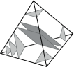
Figure 1. Normal triangles and quadrilaterals in a tetrahedron

For any vertex $v$ of the triangulation $\mathcal{T}$, the link of $v$ can be expressed as a normal surface containing only triangles (i.e., no quadrilaterals). If we say that a normal surface $S$ is the link of $v$, then we mean more precisely that $S$ is of this form. Note that, as a normal surface, the link of $v$ is unique up to normal isotopy. More generally, we say that a normal surface $S$ is vertex linking if it contains only triangles, or equivalently if $S$ is a (possibly empty) union of vertex links.

If $\mathcal{T}$ contains $n$ tetrahedra, then a normal surface in $\mathcal{T}$ can be specified by a non-negative vector in $\mathbb{Z}^{7n}$ (called standard coordinates), or by a non-negative vector in $\mathbb{Z}^{3n}$ (called quadrilateral coordinates). The vector in standard coordinates defines the surface up to normal isotopy, and the vector in quadrilateral coordinates defines the surface up to normal isotopy and addition / subtraction of vertex links. In each coordinate system we identify a finite “basis” of normal surfaces from which all others can be generated; essentially these correspond to extreme rays of a polyhedral cone [23]. The basis surfaces in each coordinate system are called standard vertex normal surfaces and quadrilateral vertex normal surfaces respectively.

For compact manifolds, the quadrilateral vertex normal surfaces are a strict subset of the standard vertex normal surfaces, are typically much faster to compute, and in many settings contain representatives of those surfaces that are “topologically interesting”. In ideal triangulations, the quadrilateral vertex normal surfaces can be much slower to compute, there may be many more of them, and they often contain non-compact spun-normal surfaces with infinitely many triangles, which we explicitly disallow in this paper. See [7] for further details on the combinatorial and computational relationships between the two systems.

2.4. Barrier surfaces

Let $M$ be a compact 3-manifold with boundary, and let $\mathcal{T}$ be an ideal triangulation of the non-compact interior $M^{\circ}$. Given any embedded closed surface $S\subset M^{\circ}$, there is a well-known normalisation process that converts $S$ into a normal surface $N\subset\mathcal{T}$.

The normal surface $N$ is obtained from $S$ by a series of isotopies, compressions, and deletion of trivial sphere components. The compressions may or may not be trivial (i.e., we might compress along curves that are trivial in the surface). Any sphere components that are deleted must be trivial (i.e., must bound a ball in $M^{\circ}$). The resulting normal surface $N$ might be disconnected, and might even be empty. See [24, Section 3.1] for a more detailed summary of the normalisation process.

Normalisation can, in some cases, make widespread changes to the original surface $S$. The barrier surface technology of Jaco and Rubinstein allows us to limit the scope of these changes, and thus retain more precise control over the relationship between $S$ and $N$. Here we outline just those parts of the theory that we need here; for the full theory the reader is referred to [24, Section 3.2].

Let $B$ be an embedded closed surface in $\mathcal{T}$, and let $C$ be some connected component of the complement $M^{\circ}\backslash B$. We say that $B$ is a barrier surface for $C$ if any embedded closed surface in $C$ can be normalised entirely within $C$. In other words, when we normalise any closed surface $S\subset C$, the normalisation process never isotopes the surface past the “barrier” $B$, and never compresses along a disc that cuts through $B$.

Often the component $C$ of $M^{\circ}\backslash B$ is clear from context (e.g., because it contains the surface $S$ that we are attempting to normalise). In this case we simply say that $B$ is a barrier surface. Amongst other examples, Jaco and Rubinstein show that all of the following are barrier surfaces [24, Theorem 3.2]:

• The boundary $B$ of a small regular neighbourhood of a subcomplex $\mathcal{K}$ of $\mathcal{T}$. Here the component $C$ of $M^{\circ}\backslash B$ must be some component not meeting the subcomplex $\mathcal{K}$. We often abuse terminology here and simply refer to $\mathcal{K}$ itself as a “barrier to normalisation”. Important examples are where $\mathcal{K}$ is a vertex of $\mathcal{T}$, or a single edge of $\mathcal{T}$.

• The boundary $B$ of a small regular neighbourhood of a normal surface $F\subset\mathcal{T}$. Likewise, the component $C$ of $M^{\circ}\backslash B$ must be some component not meeting the normal surface $F$, and we often simply refer to $F$ itself as a “barrier to normalisation”.

• A combination of the two cases above. Specifically, let $F\subset\mathcal{T}$ be a normal surface, let $\mathcal{T}^{\prime}$ be the cell decomposition induced by splitting $\mathcal{T}$ along $F$ (so $\mathcal{T}$ may contain truncated tetrahedra, triangular or quadrilateral prisms, and/or other non-tetrahedron pieces), and let $\mathcal{K}$ be a subcomplex of $\mathcal{T}^{\prime}$. Then the boundary $B$ of a small regular neighbourhood of $F\cup\mathcal{K}$ is a barrier surface. Once more the component $C$ of $M^{\circ}\backslash B$ must not meet $F\cup\mathcal{K}$, and we often refer to $F\cup\mathcal{K}$ itself as a “barrier to normalisation”.

  An example of such a barrier in this paper appears in the proof of Theorem 3.6, where $F$ is a normal sphere and $\mathcal{K}$ is a fragment of an edge of $\mathcal{T}$ that joins $F$ to a vertex of $\mathcal{T}$. A more complex example appears in the proof of Lemma 3.3, where the subcomplex $\mathcal{K}$ is an annulus or Möbius band embedded in the 2-skeleton of $\mathcal{T}$ whose boundary runs along the normal surface $F$.

2.5. Crushing normal surfaces

Many topological algorithms require us to cut a triangulation open along a normal surface. The problem with this operation is that it can be extremely expensive: the number of tetrahedra in the triangulation may grow exponentially as a result.

Jaco and Rubinstein introduce an alternative operation, called crushing [24, Section 4]. This has the advantage that the number of tetrahedra never increases (and indeed, strictly decreases if the surface is non-trivial). The disadvantage, however, is that the crushing operation can have unintended topological side-effects. Here we give a very brief outline of the operation and its effects in our setting; see [24] for full details or [10] for a simplified treatment.

Let $M$ be a compact 3-manifold with boundary, let $\mathcal{T}$ be an ideal triangulation of the non-compact interior $M^{\circ}$, and let $S$ be a two-sided normal surface in $\mathcal{T}$. To crush $S$ in $\mathcal{T}$, we perform the following steps:

Figure 2. Cutting along $S$ and collapsing the resulting boundaries

Figure 3. Different types of cells obtained after collapsing

1. We cut $\mathcal{T}$ open along the surface $S$ and collapse the two resulting boundary components to points (Figure 2). This splits each tetrahedron of $\mathcal{T}$ into a collection of cells, each of which is either a tetrahedron, a three-sided football, a four-sided football, or a triangular purse (Figure 3).

   

   

   

   Figure 4. Flattening non-tetrahedron cells

   

   (a) Dangling edges and 2-faces are removed

   

   (b) Pinched tetrahedra fall apart

   Figure 5. Cleaning up after crushing

2. We simultaneously flatten all footballs to edges and all triangular purses to triangular faces (Figure 4). Any “dangling” edges or 2-faces that do not belong to any tetrahedra are simply removed (Figure 5(a)), and any tetrahedra that are “pinched” along edges or vertices simply fall apart (Figure 5(b)).

The result will be a new generalised triangulation (possibly disconnected or possibly even empty), and the topological type of this triangulation is unclear:

• The topological effect of step (1) is simple to analyse. If $S$ is a sphere, then step (1) effectively cuts along $S$ and fills the two new boundary spheres with balls. Otherwise step (1) cuts along $S$ and converts the two new boundary components to ideal vertices, effectively producing an “ideal cell decomposition” of the non-compact manifold $M^{\circ}\backslash S$.

• Step (2) is more problematic. In general, flattening footballs and triangular purses can further change the topology, and might even introduce invalid edges. Although the “damage” can be contained in some special cases (such as crushing discs or spheres in compact manifolds [10, 24]), in general one must be very careful about drawing any conclusions about the topology of the final triangulation.

(a) Flattening a triangular pillow

(b) Flattening a bigonal pillow

(c) Flattening a bigon

Figure 6. The three atomic operations

To help understand the potential effect of step (2), we can use the crushing lemma [10]. The crushing lemma shows that, instead of simultaneously flattening all footballs and purses in step (2), we can replace this with a sequence of zero or more of the following “atomic operations”, all illustrated in Figure 6: (i) flattening triangular pillows to triangular faces; (ii) flattening bigonal pillows to bigon faces; and (iii) flattening bigon faces to edges. As before, we remove dangling edges or 2-faces and allow pinched tetrahedra to fall apart, as seen in Figure 5. The result is that we can analyse the topological effect of step (2) inductively, simply by studying the possible effect of each individual atomic move.

A final observation is that each tetrahedron of the original triangulation $\mathcal{T}$ gives rise to at most one tetrahedron in the final triangulation after crushing, and so the total number of tetrahedra does not increase. More precisely, the tetrahedra of $\mathcal{T}$ that “survive” through to the final triangulation are precisely those tetrahedra that meet the normal surface $S$ only in triangles (i.e., no quadrilaterals). In particular, if $S$ is not vertex linking (i.e., $S$ contains at least one quadrilateral piece), then the final triangulation will contain strictly fewer tetrahedra than $\mathcal{T}$.

3. Minimal triangulations of cusped hyperbolic manifolds

Here we prove a series of simple combinatorial conditions that must be satisfied by any minimal ideal triangulation of a cusped finite-volume hyperbolic 3-manifold: there can be no internal vertices (Theorem 3.5), no normal 2-spheres (Theorem 3.6), only limited normal tori or Klein bottles (Theorem 3.7), and no low-degree edges (Theorem 3.8).

Orientable variants of the first two results (no internal vertices or normal 2-spheres) were proven by Jaco and Rubinstein [24]; here we extend these to the non-orientable setting.

The fourth result (no low-degree edges) is claimed by Hildebrand and Weeks but without proof [21]. Although this is easily shown for geometric triangulations (the focus of the Hildebrand-Weeks census), significant complications arise in the general case that are not resolved in the literature. We give a full proof here.

Recall from Section 2 that, if $M^{\circ}$ is a cusped finite-volume hyperbolic 3-manifold, then any properly embedded annulus in the compact manifold $M$ that is $\pi_{1}$-injective must be boundary-parallel. We begin by recasting this fact into a more convenient form.

Observation 3.1.

Let $M$ be a compact 3-manifold with boundary whose interior $M^{\circ}$ is a cusped finite-volume hyperbolic 3-manifold. Then:

• any properly embedded annulus in $M$ must be two-sided, and must either be boundary-parallel or have boundary curves that are both trivial in $\partial M$;

• any properly embedded Möbius band in $M$ must be two-sided and boundary-parallel.

Proof.

First we note that any boundary-parallel surface must be two-sided. Now suppose that $S\subset M$ is a properly embedded annulus or Möbius band that is not boundary-parallel.

If $S$ is an annulus, then we know from Section 2.2 that $S$ cannot be $\pi_{1}$-injective. Therefore the two curves of $\partial S$ are trivial in $M$, and since $M$ has no essential compression discs they must be trivial in $\partial M$ as well. Moreover, it follows from this that $\partial S$ must be two-sided in $\partial M$, and thus $S$ is two-sided in $M$.

If $S$ is a one-sided Möbius band, let $T$ be the double of $S$ (i.e., the frontier of a regular neighbourhood of $S$ in $M$). Then $T$ is a two-sided annulus, and by the argument above either (i) $T$ is boundary-parallel, or (ii) the curves of $\partial T$ are trivial in $\partial M$. Case (i) implies that $M$ is a twisted $I$-bundle over the Möbius band (i.e., a solid torus), contradicting our assumptions on $M$. In case (ii), each boundary curve of $\partial T$ is parallel to $\partial S$ in $\partial M$; therefore $\partial S$ bounds a disc $D\subset\partial M$ and $M$ contains an embedded projective plane $D\cup S$, again a contradiction.

If $S$ is a two-sided Möbius band, then $M$ must be non-orientable. Here we apply our earlier results to the orientable double cover $\tilde{M}$ of $M$, where $S$ lifts to a two-sided annulus $\tilde{S}$. Either (i) $\tilde{S}$ is boundary-parallel in $\tilde{M}$, in which case $S$ is boundary-parallel in $M$; or (ii) the curves of $\partial\tilde{S}$ are trivial in $\partial\tilde{M}$, in which case $\partial S$ bounds a disc in $\partial M$ and we obtain an embedded projective plane as before. ∎

For the next result we require the notion of an outermost normal surface:

Definition 3.2.

Let $\mathcal{T}$ be an ideal 3-manifold triangulation, let $v$ be an ideal vertex of $\mathcal{T}$, and $S$ be a normal surface in $\mathcal{T}$ that is isotopic to the boundary of a small regular neighbourhood of $v$. We refer to such a surface as boundary-parallel to $v$.

We say that $S$ is outermost with respect to $v$ if, for any normal surface $S^{\prime}$ that is isotopic to $S$ and disjoint from $S$, either $S^{\prime}$ lies inside the collar between $S$ and a small neighbourhood of $v$, or else $S^{\prime}$ is normally isotopic to $S$.

Essentially, being outermost means that the only isotopic normal surfaces strictly further away from $v$ are “copies” of the same normal surface, formed from the same combination of triangles and/or quadrilaterals.

The following lemma is our main helper tool for proving properties of minimal triangulations. Note that Jaco and Rubinstein use a related technique in the orientable setting; see in particular [24, Theorem 7.4].

Lemma 3.3.

Let $M$ be a compact 3-manifold with boundary whose interior $M^{\circ}$ is a cusped finite-volume hyperbolic 3-manifold. Let $\mathcal{T}$ be an ideal triangulation of $M^{\circ}$, and let $v$ be an ideal vertex of $\mathcal{T}$. If $S$ is a normal surface in $\mathcal{T}$ that is boundary-parallel onto $v$ and outermost with respect to $v$, then if we crush $S$ as described in Section 2.5, some component of the resulting triangulation will also be an ideal triangulation of $M^{\circ}$.

Proof.

Recall from Section 2.5 that, by the crushing lemma, the full crushing process can be realised via the following steps:

1. cutting $\mathcal{T}$ open along $S$ and then collapsing both copies of $S$ on the boundary to points, which gives a cell decomposition formed from tetrahedra, three-sided footballs, 4-sided footballs and/or triangular purses;

2. performing a sequence of atomic operations, each of which either flattens a triangular pillow to a triangle, flattens a bigonal pillow to a bigon, or flattens a bigon to an edge.

After step (1) (cutting along $S$ and collapsing the boundaries), we obtain a cell decomposition with two components: one represents the non-compact manifold $M^{\circ}$, and one represents the non-compact product $S\times(0,1)$. These are “ideal cell decompositions” in the same sense as an ideal triangulation—if we remove the vertices whose links are non-spheres, then the underlying topological spaces are homeomorphic to $M^{\circ}$ and $S\times(0,1)$ respectively.

At this stage we throw away the $S\times(0,1)$ component, and focus solely on the ideal cell decomposition of $M^{\circ}$.

What remains is to inductively show that, if we apply any individual atomic operation of step (2) to an ideal cell decomposition of $M^{\circ}$, we obtain another ideal cell decomposition of $M^{\circ}$ (possibly after throwing away more unwanted components). We consider each type of operation in turn; the reader may wish to refer back to Figure 6 for illustrations of these operations.

• Flattening a triangular pillow:

  If the two triangular faces of the pillow are not identified in the cell decomposition then this operation does not change the topology.

  If the two faces are identified then the pillow forms an entire connected component, and therefore represents the entire ideal cell decomposition of $M^{\circ}$. Here we obtain a contradiction: by enumerating all six ways in which the upper face can be identified to the lower, we see that the underlying manifold must instead be $S^{3}$ or $L(3,1)$, or else the cell decomposition must have invalid edges.

• Flattening a bigonal pillow:

  As before, if the two bigon faces of the pillow are not identified in the cell decomposition then this operation does not change the topology.

  If the two bigon faces are identified then again the pillow must form the entire ideal cell decomposition of $M^{\circ}$, and again we obtain a contradiction. There are four ways in which the upper face can be identified to the lower, and these yield $S^{3}$, $\mathbb{R}P^{3}$, $\mathbb{R}P^{2}\times(0,1)$, or a cell decomposition with invalid edges.

• Flattening a bigon:

  Once again, if the two edges of the bigon are not identified in the cell decomposition then this operation does not change the topology. If the edges are identified, however, then more delicate arguments are required.

  

  (a) Non-orientable

  

  (b) Orientable

  Figure 7. Identifying the two edges of a bigon

  Suppose the edges are identified so the bigon becomes a non-orientable embedded surface, as in Figure 7(a). In this case, both vertices of the bigon must be identified as a single vertex. If this is an ideal vertex of the cell decomposition then by Observation 3.1 the bigon represents a boundary-parallel Möbius band in $M$; we postpone this case for the moment. If this vertex is internal to $M^{\circ}$ then the bigon becomes an embedded projective plane, which is impossible.

  Otherwise the edges must be identified to give an orientable embedded surface, as in Figure 7(b). Here there are several cases to consider:

  • Both vertices of the bigon cannot be internal. This is because each bigon was formed in step (1) above by collapsing a copy of the surface $S$ on the boundary to a point, and so each bigon meets the ideal vertex that represents the corresponding boundary component of $M$.

    

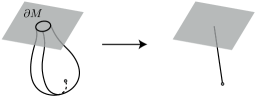
    Figure 8. Flattening a bigon that represents a disc in $M$

  • If one vertex of the bigon is internal and one is ideal, then the bigon represents a properly embedded disc in $M$. Since $M$ has no essential compression discs or essential spheres, the boundary of this disc must be trivial in $\partial M$, and so the disc and a portion of $\partial M$ must together bound a ball. Flattening the bigon has the topological effect of collapsing this ball to an edge as illustrated in Figure 8, and the result is a new ideal cell decomposition of $M^{\circ}$. The portion of the original cell decomposition that was inside the ball splits off into a separate component of the new cell decomposition, and we simply throw this component away.

    

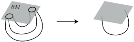
    Figure 9. Flattening a bigon that represents an annulus in $M$

  • If both vertices of the bigon are ideal, then the bigon represents a properly embedded annulus in $M$. By Observation 3.1, there are two possibilities. The annulus might be boundary-parallel in $M$; we postpone this case for the moment. Otherwise the annulus is two-sided with trivial boundary curves in $\partial M$, and again flattening the bigon has the effect of collapsing a ball to an edge as shown in Figure 9. As before, we throw away the interior of the ball, and what remains is a new ideal cell decomposition of $M^{\circ}$. Note that this argument holds even if the two ideal vertices of the bigon are identified.

The only cases not handled above are those in which a bigon of the cell decomposition represents a boundary-parallel annulus or Möbius band in $M$. To finish we show that, because our original normal surface $S$ was outermost, such cases can never occur.

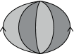
(a) Bigons in $C_{0}$

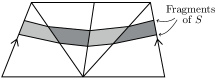
(b) Trapezoids in $\mathcal{T}$

(c) Expanding $S$ to $S^{\prime\prime}$

Figure 10. Resolving boundary-parallel annuli and Möbius bands

Let $C_{0}$ denote the ideal cell decomposition obtained immediately after cutting $\mathcal{T}$ along $S$ and collapsing the boundary components (i.e., before any atomic operations are performed). Suppose that, at some stage of the crushing process, we have a cell decomposition $C_{i}$ in which some bigon represents a boundary-parallel annulus or Möbius band. It follows that in $C_{0}$ there is a chain of one or more bigons representing this boundary-parallel annulus or Möbius band, as illustrated in Figure 10(a) (so all but one of these bigons were flattened between stages $C_{0}$ and $C_{i}$). Choose the smallest such chain of bigons, so that the corresponding annulus or Möbius band is properly embedded in $M$.

In the original triangulation $\mathcal{T}$, this chain of bigons corresponds to a chain of trapezoids, as shown in Figure 10(b): each trapezoid lives within a face of $\mathcal{T}$, and is bounded by two edge fragments of $\mathcal{T}$ and two fragments of the normal surface $S$. The union of these trapezoids forms an embedded annulus or Möbius band $Z\subset\mathcal{T}$ whose boundary $\partial Z$ runs along $S$, and which is parallel into some embedded annulus or Möbius band $Z^{\prime}\subset S$.

Let $S^{\prime}=(S\backslash Z^{\prime})\cup Z$; that is, we replace the annulus or Möbius band from within $S$ with the parallel union of trapezoids. Note that $S^{\prime}$ is isotopic to $S$. Let $S^{\prime\prime}$ be an embedded surface parallel to $S^{\prime}$ but slightly further away from the ideal vertex $v$, as illustrated in Figure 10(c). Then $S^{\prime\prime}$ is also isotopic to $S$, disjoint from $S$, and disjoint from the union of trapezoids $Z$. Moreover, both $S$ and $S^{\prime}$ lie inside the collar between $S^{\prime\prime}$ and a small neighbourhood of $v$.

We now normalise this surface $S^{\prime\prime}$; let $N$ denote the resulting normal surface in $\mathcal{T}$. Since $S^{\prime\prime}$ is boundary-parallel and $M$ has no essential compression discs, the normalised surface $N$ is again isotopic to $S$. Since $S$ and $Z$ together form a barrier to normalisation (Section 2.4), it follows that $N$ is disjoint from both $S$ and $Z$, and that $S$ still lies inside the collar between $N$ and a small neighbourhood of $v$ (i.e., the normalisation process does not “cross” through $S$). Finally, because $N$ is disjoint from the union of trapezoids $Z$, it must be a different normal surface; i.e., $N$ is not normally isotopic to the original surface $S$. This contradicts our assumption that $S$ was outermost, and the proof is complete. ∎

Corollary 3.4.

Let $M$ be a compact 3-manifold with boundary whose interior $M^{\circ}$ is a cusped finite-volume hyperbolic 3-manifold, and let $\mathcal{T}$ be a minimal ideal triangulation of $M^{\circ}$. Then the only boundary-parallel normal surfaces in $\mathcal{T}$ are vertex linking (i.e., they consist only of triangles).

Proof.

Suppose $\mathcal{T}$ has some non-vertex-linking, boundary-parallel normal surface $S$. Without loss of generality we may assume that $S$ is connected, i.e., parallel onto a single boundary component of $M$; let $v$ be the corresponding ideal vertex of $\mathcal{T}$.

There must exist a normal surface $S^{\prime}$ that is isotopic to $S$ and outermost with respect to $v$, since by a standard Kneser-type finiteness argument [26] there cannot be infinitely many disjoint normal surfaces in $\mathcal{T}$ with no pair normally isotopic. Moreover, this outermost surface $S^{\prime}$ must also be non-vertex-linking, since the original non-vertex-linking surface $S$ cannot be placed inside the collar between the vertex link of $v$ and a small neighbourhood of $v$.

It follows from Lemma 3.3 that crushing $S^{\prime}$ gives a new ideal triangulation $\mathcal{T}^{\prime}$ of $M^{\circ}$. Because $S^{\prime}$ is non-vertex linking, $\mathcal{T}^{\prime}$ must contain strictly fewer tetrahedra than $\mathcal{T}$, contradicting the minimality of $\mathcal{T}$. ∎

We can now use the results above to prove some combinatorial properties of minimal triangulations of hyperbolic manifolds.

Theorem 3.5.

Let $\mathcal{T}$ be a minimal ideal triangulation of a cusped finite-volume hyperbolic 3-manifold. Then $\mathcal{T}$ contains no internal vertices.

Proof.

Let $M$ denote the corresponding compact 3-manifold with boundary. If $\mathcal{T}$ has an internal vertex, then $\mathcal{T}$ has an edge $e$ joining some internal vertex $u$ to some ideal vertex $v$. Let $S$ be an embedded surface that bounds a small regular neighbourhood of $e$. Then $S$ is boundary-parallel onto $v$.

We now normalise $S$; let $N$ denote the corresponding normal surface in $\mathcal{T}$. Since $S$ is boundary-parallel and $M$ has no essential compression discs, $N$ must be isotopic to $S$ and therefore also boundary-parallel onto $v$. Since the edge $e$ acts as a barrier to normalisation (Section 2.4), $S$ cannot normalise to the vertex link of $v$, and so $N$ is a non-vertex-linking boundary-parallel normal surface in contradiction to Corollary 3.4. ∎

Theorem 3.6.

Let $\mathcal{T}$ be a minimal ideal triangulation of a cusped finite-volume hyperbolic 3-manifold. Then $\mathcal{T}$ contains no normal 2-spheres.

Proof.

This is essentially a variant of the proof of Theorem 3.5. Again let $M$ denote the corresponding compact 3-manifold with boundary.

If $S$ is a normal 2-sphere in $\mathcal{T}$, then $S$ must bound a ball $B$. Moreover, since every vertex of $\mathcal{T}$ is ideal (Theorem 3.5), every vertex of $\mathcal{T}$ lies outside this ball.

Let $e$ be any edge of $\mathcal{T}$ that meets $S$, let $v$ be the ideal vertex at some end of $e$, and let $\alpha\subset e$ denote the segment of $e$ that runs from $v$ along to the first point at which $e$ meets $S$.

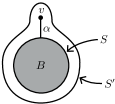
Figure 11. Extending a normal 2-sphere to a boundary-parallel surface

Let $S^{\prime}$ denote the boundary of a small regular neighbourhood of $B\cup\alpha$ in $\mathcal{T}$, as illustrated in Figure 11. Then $S^{\prime}$ is boundary-parallel onto $v$.

As before, we normalise $S^{\prime}$; let $N$ denote the corresponding normal surface in $\mathcal{T}$. Again the normalisation $N$ must also be boundary-parallel onto $v$. This time the normal surface $S$ and the arc $\alpha$ together act as a barrier to normalisation, and so once again $S^{\prime}$ cannot normalise to the vertex link of $v$. Therefore $N$ is a non-vertex-linking boundary-parallel normal surface, in contradiction to Corollary 3.4. ∎

Theorem 3.7.

Let $\mathcal{T}$ be a minimal ideal triangulation of a cusped finite-volume hyperbolic 3-manifold $M^{\circ}$. Then any non-vertex-linking normal torus or Klein bottle in $\mathcal{T}$ must bound a solid torus ($B^{2}\times S^{1}$) or solid Klein bottle ($B^{2}\stackrel{{\scriptstyle\smash{\raisebox{-2.84526pt}[0.0pt][0.0pt]{$\scriptstyle\sim$}}}}{{\times}}S^{1}$) respectively.

Proof.

Let $S$ be a non-vertex-linking normal torus or Klein bottle in $\mathcal{T}$. We take cases according to whether $S$ is a torus or Klein bottle, and whether it is two-sided or one-sided.

Suppose $S$ is a two-sided torus. By Corollary 3.4, $S$ is not boundary-parallel; since $M^{\circ}$ contains no essential tori, it follows that $S$ is not $\pi_{1}$-injective (see Section 2.2). Therefore $S$ has a compression disc $D$; that is, an embedded disc $D\subset M^{\circ}$ for which $D\cap S=\partial D$ and $\partial D$ is a non-trivial curve in $S$.

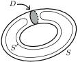
Figure 12. A compression disc for the torus $S$ and the sphere $S^{\prime}$

Let $S^{\prime}$ denote the sphere on the boundary of a regular neighbourhood of $S\cup D$, as illustrated in Figure 12. This sphere $S^{\prime}$ must bound a ball in $M^{\circ}$. If $S^{\prime}$ bounds a ball away from $S\cup D$, then the normal torus $S$ bounds a solid torus. Otherwise we can normalise $S^{\prime}$ to a normal sphere in $M^{\circ}$, since the normal torus $S$ acts a barrier to normalisation, and since the sphere $S^{\prime}$ is essential in $M^{\circ}\backslash S$. This contradicts Theorem 3.6.

Next, suppose that $S$ is a two-sided Klein bottle. Again Corollary 3.4 shows that $S$ cannot be boundary-parallel. It follows that, in the orientable double cover of $M^{\circ}$, $S$ lifts to a two-sided torus that cannot be $\pi_{1}$-injective, and so $S$ is not $\pi_{1}$-injective in $M^{\circ}$. We therefore obtain a compression disc $D\subset M^{\circ}$ for the two-sided Klein bottle $S$ as before.

As in the previous case, let $S^{\prime}$ denote the sphere on the boundary of a regular neighbourhood of $S\cup D$. Since a ball cannot contain an embedded Klein bottle, $S^{\prime}$ must bound a ball away from $S\cup D$, and therefore the normal Klein bottle $S$ bounds a solid Klein bottle.

Finally, suppose that $S$ is one-sided. Let $2S$ denote the double of $S$. Then $2S$ is a non-vertex-linking two-sided normal torus or Klein bottle, and by the arguments above $2S$ bounds a solid torus or Klein bottle in $M^{\circ}$. This is impossible, since $2S$ has the ideal vertices of $\mathcal{T}$ on one side and a twisted $I$-bundle over the torus or Klein bottle on the other. ∎

Theorem 3.8.

Let $\mathcal{T}$ be a minimal ideal triangulation of a cusped finite-volume hyperbolic 3-manifold. Then $\mathcal{T}$ has no edges of degree 1 or 2, and $\mathcal{T}$ has no edges of degree 3 that are contained in three distinct tetrahedra.

Proof.

We recall from Theorem 3.5 that every vertex of $\mathcal{T}$ is ideal. Let $n$ denote the number of tetrahedra in $\mathcal{T}$.

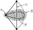
(a) Near a degree 1 edge

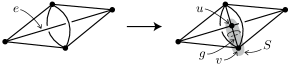
(b) Near a degree 2 edge

Figure 13. Building boundary-parallel surfaces from low-degree edges

Suppose $\mathcal{T}$ has an edge $e$ of degree 1. Then there is some tetrahedron $\Delta$ with two faces folded together around $e$, as illustrated in Figure 13(a). Let $g$ denote the edge of $\Delta$ that encircles $e$, and let $v$ denote the ideal vertex that meets $g$. Form an embedded surface $S$ that is boundary-parallel onto $v$ and that encloses the edge $g$, as shown in the illustration. Since $g$ acts a barrier to normalisation, $S$ must normalise to a surface that is boundary-parallel onto $v$ but not the vertex link of $v$, contradicting Corollary 3.4.

Suppose instead that $\mathcal{T}$ has an edge $e$ of degree 2. Then there are two tetrahedra joined together along two faces on either side of $e$, as illustrated in the left portion of Figure 13(b). We subdivide $e$ with a new internal vertex $u$, and subdivide these two original tetrahedra into four as shown in the right portion of Figure 13(b), so the resulting triangulation contains $n+2$ tetrahedra in total. Let $g$ denote one of the edges contained in all four new tetrahedra, as shown in the diagram. Let $v$ denote the ideal vertex that meets $g$, and let $S$ denote the boundary of a small regular neighbourhood of $g$. We observe that: (i) $S$ is boundary-parallel onto the ideal vertex $v$; (ii) $S$ is in fact a normal surface; and (iii) $S$ contains a quadrilateral in each of the four new tetrahedra.

Let $S^{\prime}$ be an outermost normal surface that is boundary-parallel onto $v$ and that contains $S$ in the collar between $S^{\prime}$ and $v$. As in the proof of Corollary 3.4, a standard Kneser-type finiteness argument [26] shows that such a surface $S^{\prime}$ exists (if $S$ is already outermost then $S^{\prime}$ will just be normally isotopic to $S$). It follows from Lemma 3.3 that crushing $S$ yields a new ideal triangulation $\mathcal{T}^{\prime}$ of the original manifold. Moreover, by observation (iii) above, all four of the new tetrahedra will be destroyed by the crushing process, and so $\mathcal{T}^{\prime}$ will contain at most $n-2$ tetrahedra, contradicting the minimality of $\mathcal{T}$.

Finally, suppose $\mathcal{T}$ has an edge of degree 3 contained in three distinct tetrahedra. Here we can perform a 3-2 Pachner move to reduce the number of tetrahedra, again contradicting the minimality of $\mathcal{T}$. ∎

4. Generating candidate triangulations

In this section we describe the algorithmic process of generating all candidate ideal 3-manifold triangulations with $n$ tetrahedra, for each $n=1,\ldots,9$. Here we use our combinatorial constraints on vertex links and low-degree edges (Theorems 3.5 and 3.8) as an integral part of the enumeration algorithm.

The algorithm extends earlier census algorithms in a way that is mathematically straightforward (though more intricate to code), and so we give only a brief outline of the process here. The full source code can be viewed in Regina’s online code repository [13], and will be included in the coming release of Regina 4.96.

Table 2. Generation of candidate triangulations

Tetrahedra	Triangulations
	Results of	Including low-
	Theorem 4.1	degree edges
1	1	1
2	7	18
3	31	246
4	224	3 503
5	1 075	51 652
6	6 348	810 473
7	35 312	13 090 995
8	218 476	216 484 558
9	1 313 052	3 625 523 250
Total	1 574 526	3 855 964 696

In summary, the results are:

Theorem 4.1.

Consider ideal 3-manifold triangulations in which every vertex link is a torus or Klein bottle, there are no edges of degree 1 or 2, and there are no edges of degree 3 that belong to three distinct tetrahedra. Up to relabelling, there are precisely $1\,574\,526$ such triangulations with $n\leq 9$ tetrahedra. Moreover, every minimal ideal triangulation of a cusped finite-volume hyperbolic 3-manifold with $n\leq 9$ tetrahedra belongs to this set.

Proof.

We obtain this count of $1\,574\,526$ triangulations by explicitly generating them, as outlined below in Algorithm 4.2. The middle column of Table 2 breaks this figure down by number of tetrahedra, and Section 6 lists the computational running times. It is immediate from Theorems 3.5 and 3.8 that every minimal triangulation of a cusped finite-volume hyperbolic 3-manifold belongs to this set. ∎

In brief, the enumeration algorithm operates as follows.

Algorithm 4.2.

To enumerate all generalised triangulations with $n$ tetrahedra:

1. Enumerate all connected 4-valent multigraphs on $n$ nodes (here loops and multiple edges are allowed). These will become the dual 1-skeleta, or face pairing graphs, of our triangulations—their nodes represent tetrahedra, and their arcs represent identifications between tetrahedron faces.

2. For each such multigraph $\Gamma$, recursively try all possible ways of identifying the corresponding pairs of tetrahedron faces. Note that, for each arc of $\Gamma$, there are six ways in which the corresponding pair of faces could be identified (corresponding to the six symmetries of the triangle).

To ensure that each triangulation appears only once up to relabelling, we only keep those triangulations that are “canonical”. Essentially this means that, when the pairwise face identifications are expressed as a sequence of integers, this sequence is lexicographically minimal under all possible relabellings.

To ensure that we only obtain ideal 3-manifold triangulations in which every vertex link is a torus or Klein bottle, that there are no edges of degree 1 or 2, and that there are no edges of degree 3 that belong to three distinct tetrahedra, we adapt step (2) as follows. Consider each branch of the recursion, where we have a “partially-constructed” triangulation where only some of the face identifications have been selected. We prune this branch and backtrack immediately if we can show that, no matter how we complete our triangulation, we must obtain either:

• a non-canonical triangulation;

• an invalid edge;

• an edge of degree $\leq 2$, or an edge of degree 3 that meets three distinct tetrahedra;

• a vertex link with non-zero Euler characteristic.

These pruning tests are run extremely often (the recursion tree has $6^{2n}$ branches for each multigraph $\Gamma$), and so it is imperative that they be extremely fast—a naïve implementation could ultimately slow the enumeration down even whilst reducing the size of the underlying search tree. We address this as follows:

• We construct the automorphism group of the multigraph $\Gamma$ (i.e., the group of relabellings that leave $\Gamma$ unchanged), and use this to detect situations in which any completion of our partial triangulation must be non-canonical. See [4] for details. Automorphisms have a long history of use in related combinatorial algorithms from graph theory [28].

• To detect invalid edges and low-degree edges, we track equivalence classes of tetrahedron edges (according to how they are identified within the partial triangulation), along with associated orientation information. We maintain these equivalence classes using a modification of the union-find data structure that allows not only for fast merging of equivalence classes (which union-find excels at) but also fast backtracking (which we need for our recursion). Details appear in [6].

• To detect vertex links with non-zero Euler characteristic, we likewise track equivalence classes of tetrahedron vertices, along with genus-related information. Specifically, each equivalence class represents a single vertex in the partial triangulation, and we require at all times that the link of such a vertex must be (i) a sphere with one or more punctures; (ii) a projective plane with one or more punctures; or (iii) a torus or Klein bottle with zero or more punctures.

  The paper [8] describes fast data structures based on union-find and skip lists for maintaining equivalence classes of vertices and ensuring that every vertex link is a sphere with zero or more punctures (a condition tailored for the setting of closed 3-manifolds, not ideal triangulations). It is straightforward to adapt this to our setting: for each equivalence class we now maintain the pair $(\chi,p)$, where the corresponding vertex link is a closed surface of Euler characteristic $\chi$ with $p$ punctures. Conditions (i), (ii) and (iii) simply translate to $\chi\geq 0$, with $p>0$ if $\chi>0$. The same fast data structures described in [8] can be used to update the pairs $(\chi,p)$ as we merge equivalence classes and as we backtrack.

We note that the overall framework of enumerating graphs and then gluings (i.e., the separation of steps (1) and (2) above) is common to most 3-manifold census papers in the literature. See [21, 27] for some early examples. With regard to pruning, Callahan et al. also maintain genus-related data for partially-constructed vertex links, though they give no further information on their underlying data structures [17].

The final column of Table 2 highlights the practical importance of our combinatorial results from Section 3. If we remove the constraints on low-degree edges, there are over $3.8$ billion ideal 3-manifold triangulations with $n\leq 9$ tetrahedra in which every vertex link is a torus or Klein bottle—this is several orders of magnitude more triangulations to process. Moreover, by using the low-degree edge constraint to prune the search tree (as described above), we cut the enumeration time from over 1.2 CPU years to roughly 1.4 CPU months. This highlights why such constraints should be embedded directly into the enumeration algorithm where practical, instead of using them to discard unwanted triangulations after they have been built.

5. Certifying non-hyperbolicity

We now describe the suite of algorithmic tests with which we prove Theorem 1.1 and Theorem 1.3. Our overall strategy is, for each of the $1\,574\,526$ distinct triangulations obtained in Theorem 4.1, to run a suite of tests that attempt to quickly certify one of the following: (i) that the triangulation is non-minimal and/or the underlying manifold is non-hyperbolic; or (ii) that the underlying manifold is hyperbolic and is contained in the census.

The bulk of the computational work, and the main focus of this section, is on case (i). It is important to note that we do not need to distinguish between non-minimality and non-hyperbolicity, since either allows us to discard a triangulation—even if a non-minimal triangulation represents a hyperbolic manifold, we will have processed this same manifold before. This observation simplifies some of our tests significantly.

Our suite of tests does not guarantee to certify one of the two outcomes above for every triangulation. However:

• These tests are rigorous: any results they do produce are based on exact computations, and give conclusive certificates of (i) or (ii) accordingly.

• These tests are fast: we are able to process all $1\,574\,526$ triangulations in under $16$ hours of CPU time, or $<0.04$ seconds per triangulation on average.

• These tests are effective: amongst all $1\,574\,526$ triangulations, there are just $396$ for which they do not conclusively prove (i) or (ii) above.

In the remainder of this section we describe this suite of tests in detail, with proofs of correctness where necessary. Later, in Section 6, we describe the way in which we combine these tests, give detailed running times, and wrap up the proofs of our main results (Theorem 1.1, Corollary 1.2 and Theorem 1.3). There we also explain how we handle the 396 remaining triangulations that these tests do not resolve.

We emphasise that theoretical algorithms are already known for certifying non-hyperbolicity, and indeed our tests draw upon these earlier results. The value of the tests in this paper is that they are not only correct but also fast and effective, and therefore well-suited for bulk processing with millions of triangulations as outlined above.

5.1. Local moves

Our first tests are the most elementary: we try to simplify the triangulation—that is, retriangulate the underlying manifold using fewer tetrahedra—in order to prove non-minimality. There is a trade-off here between speed and power, and so we use two different approaches: a polynomial-time greedy test, and a super-exponential-time exhaustive test. Both are based on well-known techniques.

The paper [11] describes a greedy algorithm that attempts to simplify a given 3-manifold triangulation. It is based on local modifications to the triangulation, including the standard Pachner moves (or bistellar flips) plus a variety of more complex moves. Most of these moves have been known for a long time, and have been used by many authors in a variety of settings.

The algorithm is greedy in the sense that it will never increase the number of tetrahedra at any step (i.e., it does not attempt to climb out of “wells” around local minima). As a result, it can prove triangulations to be non-minimal (and it is extremely effective at this), but it can never prove a triangulation to be minimal.

Test 5.1 (Greedy non-minimality test).

Let $\mathcal{T}$ be an ideal 3-manifold triangulation with $n$ tetrahedra. Run the greedy simplification algorithm of [11] over $\mathcal{T}$. If this results in a triangulation with fewer than $n$ tetrahedra then $\mathcal{T}$ is non-minimal.

This test is one of the fastest in our suite, with a small polynomial running time of $O(n^{4}\log n)$. See [11, Theorem 2.6] for a detailed time complexity analysis.

For triangulations where greedy methods fail, one can take a more exhaustive approach. The paper [9] describes an algorithm to enumerate all triangulations that can be reached from a given triangulation $\mathcal{T}$ by performing any sequence of 2-3 and 3-2 Pachner moves without ever exceeding a given upper limit on the number of tetrahedra. The algorithm is based on a breadth-first search, and uses isomorphism signatures to avoid revisiting the same triangulations; these are polynomial-time computable hashes that uniquely identify a triangulation up to relabelling.

Test 5.2 (Exhaustive non-minimality test).

Let $\mathcal{T}$ be an ideal 3-manifold triangulation with $n$ tetrahedra, and let $h\in\mathbb{N}$. Compute all triangulations that can be obtained from $\mathcal{T}$ by performing 2-3 and 3-2 Pachner moves without ever exceeding $n+h$ tetrahedra. If any such triangulation has fewer than $n$ tetrahedra then $\mathcal{T}$ is non-minimal.

This exhaustive test is much slower, with a super-exponential running time of $\exp(O(n\log n))$ for fixed $h$. This is still not a severe problem (in our setting, it just means that the running time is measured in seconds as opposed to microseconds). However, it does mean that we cannot run this exhaustive test over all $1\,574\,526$ triangulations; instead we must reserve it for difficult cases where simpler tests have failed.

Like the greedy test, this exhaustive test can identify non-minimal triangulations but (for any reasonable $h$) cannot prove minimality. However, it is extremely effective at simplifying triangulations that the greedy algorithm cannot, even for $h$ very small. By default we run this test with $h=2$, which in the related setting of closed manifolds is a natural threshold, and which is enough to simplify all $\sim 31$ million distinct triangulations of the 3-sphere for $n\leq 9$ [9].

5.2. Normal surfaces

As seen in Section 4, some of our combinatorial results from Section 3 can be embedded directly into the enumeration algorithm (e.g., no low-degree edges and no internal vertices). Others cannot (e.g., the constraints involving normal surfaces), and so we use these here instead as tests for non-minimality.

The following tests follow directly from Theorems 3.6 and 3.7, plus the fact that a cusped finite-volume hyperbolic 3-manifold cannot contain an embedded projective plane.

Test 5.3 (Spheres and projective planes).

Let $\mathcal{T}$ be an ideal 3-manifold triangulation. Enumerate all standard vertex normal surfaces in $\mathcal{T}$. If any of these surfaces has positive Euler characteristic, then $\mathcal{T}$ is either non-minimal or does not represent a cusped finite-volume hyperbolic 3-manifold.

Test 5.4 (Tori and Klein bottles).

Let $\mathcal{T}$ be an ideal 3-manifold triangulation. Enumerate all standard vertex normal surfaces in $\mathcal{T}$, and test whether any such surface is a torus or Klein bottle $S$ for which:

• $S$ is one-sided; or

• $S$ is two-sided, and if we cut $\mathcal{T}$ open along $S$ then no component of the resulting triangulation is a solid torus or solid Klein bottle.

If such a surface is found, then $\mathcal{T}$ is either non-minimal or does not represent a cusped finite-volume hyperbolic 3-manifold.

Test 5.4 requires us to algorithmically recognise the solid torus and solid Klein bottle. For the solid torus we use a standard crushing-based algorithm, which we describe in more detail later (Algorithm 5.8). For the solid Klein bottle we run solid torus recognition over the orientable double cover.

Regarding running times: Test 5.3 runs in time $O(7^{n}\times\mathrm{poly}(n))$—the bottleneck here is simply enumerating all standard vertex normal surfaces. See [15] for the full time complexity analysis. Test 5.4 may require doubly-exponential time in theory, since cutting along $S$ could introduce exponentially many tetrahedra. In practice however, vertex normal surfaces typically have very few normal discs [16] and so the resulting triangulations remain manageably small.

We emphasise again how our tests become simpler because we do not need to distinguish between non-minimality and non-hyperbolicity. It is enough just to find normal spheres, tori or Klein bottles as described above—there is no need to test whether these surfaces are essential (which, for tori and Klein bottles in particular, would be a more expensive process).

The tests above only examine vertex normal surfaces, not arbitrary normal surfaces. This is to make the tests fast enough for our bulk-processing requirements. For Test 5.3, this restriction does not reduce the power of the test at all—a simple linearity argument shows that $\mathcal{T}$ contains a standard vertex normal surface of positive Euler characteristic if and only if it contains any normal surface of positive Euler characteristic. For Test 5.4 we may lose some opportunities to prove non-minimality or non-hyperbolicity, but as we see later in Section 6, this does not hurt us significantly in practice.

We use standard vertex normal surfaces instead of quadrilateral vertex normal surfaces because this ensures that the vertex surfaces are closed. In ideal triangulations, quadrilateral vertex surfaces typically include non-compact spun-normal surfaces [34], which we wish to avoid here.

5.3. Seifert fibred spaces

Some Seifert fibred spaces contain no essential tori or Klein bottles at all—examples include Seifert fibred spaces over the disc, annulus or pair of pants with at most two, one and zero exceptional fibres respectively. Given an ideal triangulation of such a space that is both minimal and sufficiently “nice” (i.e., with no “unnecessary” normal spheres, tori or Klein bottles), all of the tests seen thus far will be inconclusive. The following tests aim to resolve such cases.

Our focus now is purely on certifying non-hyperbolicity (as opposed to non-minimality), and so we allow ourselves to alter the triangulation where this is more convenient. In particular, we truncate ideal vertices to obtain real boundary triangles, and for non-orientable manifolds we work in the orientable double cover.

Our first test in this section is extremely opportunistic, but also extremely fast and surprisingly effective. This uses the combinatorial recognition routines built into Regina. In essence, we examine the combinatorics of the triangulation to see if it uses a standard combinatorial construction for Seifert fibred spaces, and if it does, we simply “read off” the Seifert fibred space parameters to identify the underlying 3-manifold.

In brief, the standard construction involves (i) starting with a minimal triangulation of a punctured surface $F$; (ii) expanding each triangle of the surface into a 3-tetrahedron triangular prism, giving a triangulation of $F\times I$; (iii) gluing the two ends of each prism together, which converts this into $F\times S^{1}$; and then (iv) attaching layered solid tori to some of the remaining torus boundary components to provide the exceptional fibres.

The reason combinatorial recognition is effective is because, after we simplify a triangulation of a Seifert fibred space using the greedy algorithm from Test 5.1, the result is often found to be a standard construction of this type. See [11] for further discussion of Regina’s combinatorial recognition facilities.

Test 5.5 (Combinatorial recognition).

Let $\mathcal{T}$ be an ideal 3-manifold triangulation. Truncate the ideal vertices of $\mathcal{T}$, and switch to the orientable double cover if $\mathcal{T}$ is non-orientable. Simplify the resulting triangulation using the greedy algorithm of Test 5.1. If the result is a standard construction of a Seifert fibred space as outlined above, then $\mathcal{T}$ does not represent a cusped finite-volume hyperbolic 3-manifold.

The test above is fast because every step (truncation, double cover, greedy simplification and combinatorial recognition) runs in small polynomial time [11].

The next test is significantly more expensive, but it can succeed where combinatorial recognition fails. Here we explicitly search for a normal annulus that:

• for a Seifert fibred space $M$ over the disc with $\leq 2$ exceptional fibres, splits $M$ into a pair of solid tori;

• for a Seifert fibred space $M$ over the annulus with $\leq 1$ exceptional fibre, splits $M$ open into a single solid torus;

• for a Seifert fibred space $M$ over the pair of pants with no exceptional fibres, splits $M$ into a pair of products $\mathrm{Torus}\times I$.

As with our earlier normal surface tests, we restrict our search to vertex normal surfaces. This time we work with quadrilateral vertex surfaces, since for manifolds with boundary triangles there are typically far more standard vertex surfaces than quadrilateral vertex surfaces, and the “important” surfaces typically appear in both sets. As before, this restriction is primarily designed to keep the test fast—it may cause us to lose opportunities to recognise Seifert fibred spaces, but we see in Section 6 that this does not hurt us in practice.

Test 5.6 (Annuli and Möbius bands).

Let $\mathcal{T}$ be an ideal 3-manifold triangulation. Truncate the ideal vertices of $\mathcal{T}$, and switch to the orientable double cover if $\mathcal{T}$ is non-orientable. Simplify the resulting triangulation using the greedy algorithm of Test 5.1, and denote the resulting triangulation by $\mathcal{T}^{\prime}$.

Now enumerate all quadrilateral vertex normal surfaces in $\mathcal{T}^{\prime}$. If such a surface $S$ satisfies any of the following conditions, then the original triangulation $\mathcal{T}$ does not represent a cusped finite-volume hyperbolic 3-manifold:

1. $S$ is a Möbius band;

2. $S$ is an annulus, $\mathcal{T}^{\prime}$ has precisely one boundary component, and if we cut $\mathcal{T}^{\prime}$ open along $S$ then we obtain two solid tori;

3. $S$ is an annulus, $\mathcal{T}^{\prime}$ has precisely two boundary components, and if we cut $\mathcal{T}^{\prime}$ open along $S$ then we obtain one solid torus (and nothing else);

4. $S$ is an annulus, $\mathcal{T}^{\prime}$ has precisely three boundary components, and if we cut $\mathcal{T}^{\prime}$ open along $S$ then we obtain two triangulations of the product $\mathrm{Torus}\times I$.

We give a proof of correctness shortly, but first some implementation details:

• Like Test 5.4 before, this test requires us to recognise the solid torus. This we do using the standard crushing-based algorithm outlined below (Algorithm 5.8), and the result is guaranteed to be conclusive.

• This test also requires us to recognise $\mathrm{Torus}\times I$. This we do using combinatorial recognition, as outlined earlier in Test 5.5. The result might be inconclusive (i.e., we cannot tell whether a triangulation represents $\mathrm{Torus}\times I$ or not), but in such a case we simply abandon the current annulus $S$ and move on to the next vertex normal surface. Again we are making a trade-off: using combinatorial recognition to test for $\mathrm{Torus}\times I$ keeps the test fast but may come with an opportunity cost, yet again we see in Section 6 that this trade-off does not appear to hurt us in practice.

Proof for Test 5.6.

Let $M^{\circ}$ denote the underlying non-compact manifold for $\mathcal{T}$, and suppose that $M^{\circ}$ is a cusped finite-volume hyperbolic 3-manifold. Let $M^{\prime}$ denote the compact orientable manifold represented by $\mathcal{T}^{\prime}$, and suppose that the normal annulus or Möbius band $S\subset M^{\prime}$ satisfies one of the conditions (1)–(4) above.

By Observation 3.1, the orientable manifold $M^{\prime}$ cannot contain a properly embedded Möbius band at all; that is, condition (1) is impossible. Therefore $S$ must be an annulus. If $S$ is boundary-parallel then we must be in case (2) and $M^{\prime}$ itself must also be a solid torus, contradicting hyperbolicity.

Therefore $S$ is not boundary-parallel, and so (by Observation 3.1 again) $S$ is an annulus whose boundary curves are trivial in $\partial M^{\prime}$. Taking cases (2)–(4) separately:

• Case 2: Suppose $M^{\prime}$ has one boundary component and $S$ separates $M^{\prime}$ into a pair of solid tori. The only way to arrange this is for the two trivial curves of $\partial S$ to sit one inside the other on $\partial M^{\prime}$, as shown in Figure 14(a). In this case $M^{\prime}$ is obtained by attaching the two solid tori along an annulus that is trivial on one torus boundary but non-trivial on the other; this makes $M^{\prime}$ a connected sum of the solid torus with one of $S^{3}$, $S^{2}\times S^{1}$ or a lens space, any of which contradicts hyperbolicity.

• Case 3: Suppose $M^{\prime}$ has two boundary components and $S$ cuts $M^{\prime}$ open into a single solid torus $T$. This is impossible, since if $\partial S$ consists of trivial curves on $\partial M^{\prime}$ then cutting $M^{\prime}$ open along $S$ will always leave at least two boundary components.

  

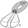
  (a) One boundary component

  

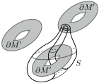
  (b) Three boundary components

  Figure 14. Resolving cases (2) and (4) of Test 5.6

• Case 4: Suppose $M^{\prime}$ has three boundary components and $S$ splits $M^{\prime}$ into a pair of $\mathrm{Torus}\times I$ pieces. The only way to arrange this is for the two trivial curves of $\partial S$ to sit one inside the other on some component of $\partial M^{\prime}$, as shown in Figure 14(b). Now $M^{\prime}$ is now obtained by attaching the two $\mathrm{Torus}\times I$ pieces along an annulus that is trivial on one $\mathrm{Torus}\times I$ boundary but non-trivial on the other; this makes $M^{\prime}$ a connected sum of the solid torus with $\mathrm{Torus}\times I$, contradicting hyperbolicity once more. ∎

Our final test for non-hyperbolicity is a special case, but one for which we have an algorithm that is always conclusive and (despite requiring theoretical exponential time) fast in practice:

Test 5.7 (Solid torus recognition).

Let $\mathcal{T}$ be an ideal 3-manifold triangulation. Truncate the ideal vertices of $\mathcal{T}$, and switch to the orientable double cover if $\mathcal{T}$ is non-orientable. If the resulting triangulation represents the solid torus, then $\mathcal{T}$ does not represent a cusped finite-volume hyperbolic 3-manifold.

Solid torus recognition features repeatedly throughout this suite of tests (see Tests 5.4, 5.6 and 5.7), and so we outline the algorithm below. This algorithm does not appear in the literature, but it is a straightforward assembly of well-known components: the overall crushing framework is due to Jaco and Rubinstein [24], and the branch-and-bound search for normal discs and spheres is due to the author and Ozlen [14].

Algorithm 5.8.

Let $\mathcal{T}$ be a 3-manifold triangulation with boundary triangles (i.e., not an ideal triangulation). To test whether or not $\mathcal{T}$ represents the solid torus:

• Check that $\mathcal{T}$ is orientable with $H_{1}=\mathbb{Z}$ and a single torus boundary component. If not, then $\mathcal{T}$ is not the solid torus.

• Repeatedly search for non-vertex-linking normal surfaces of positive Euler characteristic, and crush them as described in Section 2.5. Then $\mathcal{T}$ represents the solid torus if and only if, after crushing, the resulting triangulation is a (possibly empty) disjoint union of 3-spheres and/or 3-balls.

The bottleneck of this algorithm is the search for non-vertex-linking normal surfaces of positive Euler characteristic (although 3-sphere and 3-ball recognition are non-trivial, they too reduce to this same bottleneck). For this step we use the branch-and-bound framework described in [14]: essentially we work through a hierarchy of linear programs that, in many experiments, is seen to prune the exponential search tree down to linear size.

Proof for Algorithm 5.8.

The arguments are standard, and so we merely sketch the proof here.

The algorithm terminates because each crushing operation reduces the total number of tetrahedra. Correctness follows from two observations: (i) that any solid torus must contain a normal meridional disc [20]; and (ii) when crushing a disc or sphere in an orientable and non-ideal triangulation, the only possible topological side-effects (beyond cutting along and collapsing the original disc or sphere) are cutting along additional discs or spheres, filling boundary spheres with balls, and/or deleting entire $B^{3}$, $S^{3}$, $\mathbb{R}P^{3}$ or $L_{3,1}$ components [24].

It follows that repeatedly crushing spheres and discs in the solid torus must leave us with a disjoint union of 3-spheres and/or 3-balls, but if we start with some different manifold with torus boundary and $\mathbb{Z}$ homology then we must have some different topological component left over. ∎

5.4. Hyperbolic manifolds

This concludes our suite of non-hyperbolicity and non-minimality tests; all that remains is to certify that the remaining manifolds are hyperbolic and (for $n\leq 8$ tetrahedra) to locate them in the Callahan-Hildebrand-Thistlethwaite-Weeks census. For this we call upon pre-existing software: we ask SnapPea to find hyperbolic structures and HIKMOT to rigorously verify them.

To account for the fact that we may encounter non-geometric triangulations of hyperbolic manifolds, we call upon SnapPea’s built-in “randomisation” routine, which randomly performs a sequence of local moves (e.g., Pachner moves) to obtain a different triangulation of the same manifold (hopefully one that is geometric).

Our hyperbolicity test is simple: we identify all of those triangulations that we suspect to be hyperbolic (using SnapPea), group these into classes of triangulations that represent the same manifold (using their Epstein-Penner decompositions), and use HIKMOT to rigorously certify that at least one triangulation in each class is geometric. The details are as follows.

Test 5.9 (Hyperbolicity test with $r$ randomisations).

Let $\mathcal{T}$ be an ideal 3-manifold triangulation, and let $r\in\mathbb{N}$. We ask SnapPea to find a complete hyperbolic structure on $\mathcal{T}$. If this fails, we make up to $r$ additional attempts in which we ask SnapPea to randomise the triangulation and try again.

If at any attempt SnapPea does find a complete hyperbolic structure then we stop, ask SnapPea to compute the corresponding Epstein-Penner decomposition $\mathcal{D}$, and ask HIKMOT to attempt to rigorously verify that the corresponding triangulation is geometric. We then record the original input triangulation $\mathcal{T}$, the Epstein-Penner decomposition $\mathcal{D}$, and whether HIKMOT’s verification was successful. If all attempts to find a complete hyperbolic structure fail, then we declare the test inconclusive for $\mathcal{T}$.

For each Epstein-Penner decomposition $\mathcal{D}$ that we record, let $\mathcal{T}_{1},\ldots,\mathcal{T}_{k}$ be the (possibly many) input triangulations from which it was obtained. If HIKMOT’s verification succeeded for any of these $\mathcal{T}_{i}$, then we declare that all of these $\mathcal{T}_{i}$ represent a hyperbolic manifold. Otherwise the test is inconclusive for all of $\mathcal{T}_{1},\ldots,\mathcal{T}_{k}$.

We recall that SnapPea’s complete hyperbolic structures are merely approximations computed using inexact floating-point arithmetic, and that its Epstein-Penner decompositions may or may not be correct. Nevertheless, we can prove that our declarations of hyperbolicity are rigorous:

Proof.

Consider some class $\mathcal{T}_{1},\ldots,\mathcal{T}_{k}$ for which SnapPea computes a common Epstein-Penner decomposition $\mathcal{D}$, and for which HIKMOT certifies some $\mathcal{T}_{i}$ to be geometric. Although SnapPea might not have computed the Epstein-Penner decompositions correctly, it nevertheless computes these decompositions using Pachner moves [36], and so we can still guarantee that $\mathcal{T}_{1},\ldots,\mathcal{T}_{k}$ represent the same manifold. It follows that, since HIKMOT has certified hyperbolicity for one of the $\mathcal{T}_{i}$, then all of the $\mathcal{T}_{i}$ represent this same hyperbolic manifold. ∎

Note that SnapPea itself has a mechanism to automatically randomise triangulations (up to $64$ times) when attempting to find a complete hyperbolic structure. We disable this feature here, and instead allow a much smaller number of retriangulations (by default, $r=8$). This is to keep the test reasonably fast for triangulations that represent non-hyperbolic manifolds (the vast majority of cases), for which SnapPea will fail on all $r$ retriangulations and the test will always be inconclusive.

6. Building and processing the census

Here we briefly outline how we organise the computations, deal with the handful of unresolved cases, and finalise the proof of our main results (Theorem 1.1, Corollary 1.2 and Theorem 1.3).

Table 3. Running the tests of Section 5 over all enumerated triangulations

# Tetrahedra	1	2	3	4	5	6	7	8	9
Test 5.1: Greedy non-
minimality test	$-$	$-$	$-$	25	268	2 224	16 622	130 951	902 439
Test 5.9: Hyperbolicity
(no randomisations)	1	5	21	136	548	2 647	11 341	48 437	204 139
Test 5.3: Spheres and
projective planes	$-$	$-$	$-$	$-$	$-$	$-$	17	203	1 430
Test 5.9: Hyperbolicity
($r=8$ randomisations)	$-$	$-$	$-$	$-$	4	52	360	1 974	11 608
Test 5.4: Tori and Klein
bottles	$-$	2	10	63	253	1 379	6 666	35 338	186 104
Test 5.5: Combinatorial
recognition	$-$	$-$	$-$	$-$	$-$	6	10	75	417
Test 5.2: Exhaustive non-
minimality ($h=2$)	$-$	$-$	$-$	$-$	2	40	293	1 427	6 195
Test 5.6: Annuli and
Möbius bands	$-$	$-$	$-$	$-$	$-$	$-$	$-$	32	366
Test 5.7: Solid torus
recognition	$-$	$-$	$-$	$-$	$-$	$-$	$-$	$-$	$-$
Unresolved	$-$	$-$	$-$	$-$	$-$	$-$	3	39	354
Total	1	7	31	224	1 075	6 348	35 312	218 476	1 313 052

For each of the $1\,574\,526$ triangulations that we enumerate in Theorem 4.1, we run the tests of Section 5 in the order shown in Table 3. This table also shows how many cases each test resolves. Once a triangulation is certified as either (i) non-minimal and/or non-hyperbolic or (ii) hyperbolic, then we do not run any further tests on it (i.e., we expect the numbers towards the bottom of Table 3 to be small, since very few cases remain by that stage).

As a rough guide, the tests are ordered so that (i) faster tests are placed before slower tests; and (ii) tests that are likely to resolve many cases are placed earlier. For example, the polynomial-time greedy non-minimality test is placed well before the super-exponential-time exhaustive non-minimality test, and tests that require building a truncated orientable double cover (which could increase the number of tetrahedra significantly) are placed towards the end. Solid torus recognition is placed last, since in practice one finds that most triangulations of the solid torus are easy to simplify, and are therefore caught by the polynomial-time greedy non-minimality and/or combinatorial recognition tests.

As seen in Table 3, the full suite of tests leaves just $396$ of the $1\,574\,526$ triangulations unresolved. For these $396$ cases:

• 4 were cases that crashed SnapPea during the initial run. Rerunning them (with a different random seed) shows them to be hyperbolic (Test 5.9).

• The remaining cases are resolved by an exhaustive search through different triangulations of the same manifold. As in Test 5.2, we try all possible combinations of 2-3 and 3-2 Pachner moves without exceeding $h$ additional tetrahedra. For $h=3$, this certifies 175 as hyperbolic (by producing a new triangulation that we had already certified as such), and 166 as non-minimal (by producing a new triangulation with fewer tetrahedra). Of the 51 leftover cases, rerunning with $h=4$ certifies 1 as hyperbolic and the final 50 as non-minimal.

The overall result is that $281\,453$ of the original $1\,574\,526$ triangulations are certified to represent cusped finite-volume hyperbolic 3-manifolds, and all others are certified as non-minimal and/or non-hyperbolic. At this stage we partition our triangulations into classes that represent the same manifold:

• Test 5.9 records the Epstein-Penner decomposition computed by SnapPea for each triangulation. Although these Epstein-Penner decompositions might be incorrect, it is guaranteed that triangulations that produce the same cell decomposition represent the same manifold, and so we can group them together as such. This produces exactly $76\,000$ manifold classes.

• From each triangulation we run yet another exhaustive search through 2-3 and 3-2 Pachner moves (without exceeding $h=2$ additional tetrahedra) in order to identify classes that should be merged—this is necessary because SnapPea does indeed compute some Epstein-Penner decompositions incorrectly. This reduces our $76\,000$ manifold classes down to the final list of $75\,956$.

• We discard any triangulation that does not use the fewest tetrahedra in its class (since these are clearly non-minimal). This cuts our list of $281\,453$ hyperbolic triangulations down to the final list of $229\,112$ triangulations.

We emphasise that there is still no guarantee that our $75\,956$ manifold classes represent distinct manifolds, and therefore that our $229\,112$ triangulations are indeed minimal. This we resolve later in Section 7 using algebraic invariants.

This concludes the proof of Theorem 1.3 (that our new 9-tetrahedron census has no intruders and no omissions). To finish the proofs of Theorem 1.1 and Corollary 1.2 (that the older Callahan-Hildebrand-Thistlethwaite-Weeks census has no intruders and no omissions), we simply verify that (i) each manifold class with an $n\leq 8$-tetrahedron triangulation includes a representative from the Callahan-Hildebrand-Thistlethwaite-Weeks census; and that (ii) each manifold from this census is contained in at least one such class.

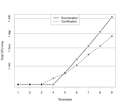
Figure 15. Running times

Figure 15 plots the total running times for both the enumeration of our $1\,574\,526$ triangulations as described in Section 4, and the certification of triangulations as non-minimal, non-hyperbolic and/or hyperbolic using the tests of Section 5. As seen in the plot, the certification time—though significant—is a mere fraction of the time required for enumeration.

This backs up our claim that the tests are fast—the bottleneck for producing a rigorous and verified cusped hyperbolic census is not the verification, but just the raw generation of candidate triangulations. Looking forward, it therefore seems entirely feasible for future extensions of the cusped hyperbolic census to be made rigorous in this way.

7. Preventing duplicates

To finish, we describe how we prove Theorem 1.4—that no two manifolds in the census are homeomorphic. For this we use algebraic invariants, which can be computed and compared exactly.

Notation.

Let $G$ be any group. We let $G^{\mathrm{ab}}$ denote the abelianisation of $G$. For any finite index $i\in\mathbb{N}$, we let $S_{i}(G)$ denote a set containing one arbitrary representative of each conjugacy class of index $i$ subgroups of $G$. Finally, we let $S_{i}^{\mathrm{ab}}(G)$ denote the multiset of abelianisations $\{s^{\mathrm{ab}}\,|\,s\in S_{i}(G)\}$; here multiset means that we record multiple occurrences of the same abelian group.

Although $S_{i}(G)$ is not well-defined (since we have a choice of representatives), the multiset of abelianisations $S_{i}^{\mathrm{ab}}(G)$ is. If $G$ is given as a finite presentation then $S_{i}^{\mathrm{ab}}(G)$ is a computable invariant of $G$, though this computation is only feasible for small indices $i$ since the running time can grow exponentially (or worse) with $i$ [32].

Lemma 7.1.

Amongst all cusped finite-volume hyperbolic 3-manifolds that can be triangulated with $n\leq 9$ ideal tetrahedra, any two distinct manifolds differ in at least one of the following invariants:

• orientability;

• the first homology $H_{1}=\pi_{1}^{\mathrm{ab}}$;

• for each index $2\leq i\leq 11$, the multiset of abelianisations $S_{i}^{\mathrm{ab}}(\pi_{1})$.

Here $\pi_{1}$ denotes, as usual, the fundamental group of a 3-manifold.

Proof.

By Theorem 1.3, our $75\,956$ census manifolds together contain all cusped finite-volume hyperbolic 3-manifolds that can be triangulated with $n\leq 9$ ideal tetrahedra (though we do not yet know whether these manifolds are distinct). We therefore prove Lemma 7.1 simply by computing the invariants above for all $75\,956$ census manifolds and observing that they partition the manifolds into $75\,956$ distinct homeomorphism classes. ∎

Theorem 1.4 now follows immediately from the computations in the proof above.

For the computations themselves we use Magma [3], which is fast and robust enough to compute hundreds of thousands of such invariants within a reasonable running time. (Other software packages such as SnapPy and GAP can also compute these invariants, but they are infeasibly slow for some problematic cases.)

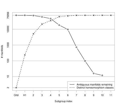
Figure 16. Proving that all $75\,956$ census manifolds are distinct

Of course we do not need to compute all such invariants for all $75\,956$ manifolds. We compute $H_{1}$, $S_{2}^{\mathrm{ab}}(\pi_{1})$, …, $S_{11}^{\mathrm{ab}}(\pi_{1})$ in 11 distinct stages (these are ordered by increasing difficulty), and after each stage we put aside those census manifolds that have been successfully distinguished from all others. Those manifolds that remain (i.e., whose invariants so far coincide with at least one other manifold) we call ambiguous manifolds, and we keep these for further processing. Figure 16 plots how many ambiguous manifolds remain after computing $S_{i}^{\mathrm{ab}}(\pi_{1})$ for each subgroup index $i$. Note that the vertical axis uses a logarithmic scale.

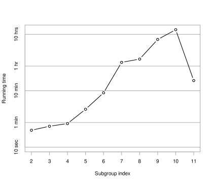
Figure 17. Running times for computing low-index subgroups

Figure 17 plots the running time required to compute $S_{i}^{\mathrm{ab}}(\pi_{1})$ for each $i$, again on a logarithmic scale (measured on a single 3.47GHz Intel Xeon CPU). This running time was only for ambiguous manifolds, as explained above; in particular, the peak time of $14$ hours for index $i=10$ was for just $16$ manifolds that remained at that late stage of processing. We are perhaps fortunate that $i=11$ was sufficient to distinguish all of the census manifolds, and that we were not required to increase the index any further.

We note that these final $16$ manifolds are difficult to distinguish even with the help of inexact floating-point invariants. They come in eight ambiguous pairs of non-orientable manifolds, where both manifolds in each pair have the same hyperbolic volume and shortest geodesic, and indeed homeomorphic orientable double covers. Examining a larger section of the length spectrum does, however, reveal enough information to distinguish them (subject to numerical error). For reference, these final eight pairs appear in the census tables as:

$$\small\begin{array}[]{llll}(\mathtt{y296},\ \mathtt{y297})&(\mathtt{n8\_0534},\ \mathtt{n8\_0535})&(\mathtt{n9\_1033},\ \mathtt{n9\_1034})&(\mathtt{n9\_1091},\ \mathtt{n9\_1092})\\ (\mathtt{n9\_1183},\ \mathtt{n9\_1184})&(\mathtt{n9\_1200},\ \mathtt{n9\_1201})&(\mathtt{n9\_2015},\ \mathtt{n9\_2016})&(\mathtt{n9\_2121},\ \mathtt{n9\_2122}).\end{array}$$

References

- [1] Colin Adams and William Sherman, Minimum ideal triangulations of hyperbolic -manifolds, Discrete Comput. Geom. 6 (1991), no. 2, 135–153.
- [2] Francis Bonahon, Geometric structures on 3-manifolds, Handbook of Geometric Topology, North-Holland, Amsterdam, 2002, pp. 93–164.
- [3] Wieb Bosma, John Cannon, and Catherine Playoust, The Magma algebra system. I. The user language, J. Symbolic Comput. 24 (1997), no. 3-4, 235–265, Computational algebra and number theory (London, 1993).
- [4] Benjamin A. Burton, Minimal triangulations and normal surfaces, Ph.D. thesis, University of Melbourne, 2003, available from http://regina.sourceforge.net/.
- [5] by same author, Introducing Regina, the 3-manifold topology software, Experiment. Math. 13 (2004), no. 3, 267–272.
- [6] by same author, Enumeration of non-orientable 3-manifolds using face-pairing graphs and union-find, Discrete Comput. Geom. 38 (2007), no. 3, 527–571.
- [7] by same author, Converting between quadrilateral and standard solution sets in normal surface theory, Algebr. Geom. Topol. 9 (2009), no. 4, 2121–2174.
- [8] by same author, Detecting genus in vertex links for the fast enumeration of 3-manifold triangulations, ISSAC 2011: Proceedings of the 36th International Symposium on Symbolic and Algebraic Computation, ACM, 2011, pp. 59–66.
- [9] by same author, The Pachner graph and the simplification of 3-sphere triangulations, SCG ’11: Proceedings of the Twenty-Seventh Annual Symposium on Computational Geometry, ACM, 2011, pp. 153–162.
- [10] by same author, A new approach to crushing 3-manifold triangulations, To appear in Discrete & Computational Geometry, arXiv:1212.1441, 2012.
- [11] by same author, Computational topology with Regina: Algorithms, heuristics and implementations, Geometry and Topology Down Under (Craig D. Hodgson, William H. Jaco, Martin G. Scharlemann, and Stephan Tillmann, eds.), Contemporary Mathematics, no. 597, Amer. Math. Soc., Providence, RI, 2013.
- [12] by same author, A duplicate pair in the SnapPea census, To appear in Experimental Mathematics, arXiv:1311.7615, November 2013.
- [13] Benjamin A. Burton, Ryan Budney, William Pettersson, et al., Regina: Software for 3-manifold topology and normal surface theory, http://regina.sourceforge.net/, 1999–2014.
- [14] Benjamin A. Burton and Melih Ozlen, A fast branching algorithm for unknot recognition with experimental polynomial-time behaviour, Preprint, arXiv:1211.1079, November 2012.
- [15] by same author, A tree traversal algorithm for decision problems in knot theory and 3-manifold topology, Algorithmica 65 (2013), no. 4, 772–801.
- [16] Benjamin A. Burton, João Paixão, and Jonathan Spreer, Computational topology and normal surfaces: Theoretical and experimental complexity bounds, ALENEX 2013: Proceedings of the Meeting on Algorithm Engineering & Experiments, SIAM, 2013, pp. 78–87.
- [17] Patrick J. Callahan, Martin V. Hildebrand, and Jeffrey R. Weeks, A census of cusped hyperbolic 3-manifolds, Math. Comp. 68 (1999), no. 225, 321–332.
- [18] Marc Culler, Nathan M. Dunfield, and Jeffrey R. Weeks, SnapPy, a computer program for studying the geometry and topology of 3-manifolds, http://snappy.computop.org/, 1991–2013.
- [19] D. B. A. Epstein and R. C. Penner, Euclidean decompositions of noncompact hyperbolic manifolds, J. Differential Geom. 27 (1988), no. 1, 67–80.
- [20] Wolfgang Haken, Theorie der Normalflächen, Acta Math. 105 (1961), 245–375.
- [21] Martin V. Hildebrand and Jeffrey R. Weeks, A computer generated census of cusped hyperbolic 3-manifolds, Computers and Mathematics (Cambridge, MA, 1989), Springer, New York, 1989, pp. 53–59.
- [22] Neil Hoffman, Kazuhiro Ichihara, Masahide Kashiwagi, Hidetoshi Masai, Shin’ichi Oishi, and Akitoshi Takayasu, Verified computations for hyperbolic 3-manifolds, Preprint, arXiv:1310.3410, October 2013.
- [23] William Jaco and Ulrich Oertel, An algorithm to decide if a -manifold is a Haken manifold, Topology 23 (1984), no. 2, 195–209.
- [24] William Jaco and J. Hyam Rubinstein, 0-efficient triangulations of 3-manifolds, J. Differential Geom. 65 (2003), no. 1, 61–168.
- [25] Michael Kapovich, Hyperbolic manifolds and discrete groups, Modern Birkhäuser Classics, Birkhäuser, Boston, MA, 2009, Reprint of the 2001 edition.
- [26] Hellmuth Kneser, Geschlossene Flächen in dreidimensionalen Mannigfaltigkeiten, Jahresbericht der Deut. Math. Verein. 38 (1929), 248–260.
- [27] Sergei V. Matveev, Tables of 3-manifolds up to complexity 6, Max-Planck-Institut für Mathematik Preprint Series (1998), no. 67, available from http://www.mpim-bonn.mpg.de/html/preprints/preprints.html.
- [28] Brendan D. McKay, Practical graph isomorphism, Proceedings of the Tenth Manitoba Conference on Numerical Mathematics and Computing, Vol. I (Winnipeg, Man., 1980), vol. 30, 1981, pp. 45–87.
- [29] Harriet Moser, Proving a manifold to be hyperbolic once it has been approximated to be so, Algebr. Geom. Topol. 9 (2009), no. 1, 103–133.
- [30] Udo Pachner, P.L. homeomorphic manifolds are equivalent by elementary shellings, European J. Combin. 12 (1991), no. 2, 129–145.
- [31] William Sherman, Hyperbolic manifolds from ideal tetrahedra, Undergraduate thesis, Williams College, 1988.
- [32] Charles C. Sims, Computation with finitely presented groups, Encyclopedia of Mathematics and its Applications, vol. 48, Cambridge University Press, Cambridge, 1994.
- [33] Morwen Thistlethwaite, Cusped hyperbolic manifolds with 8 tetrahedra, http://www.math.utk.edu/~morwen/8tet/, October 2010.
- [34] Stephan Tillmann, Normal surfaces in topologically finite 3-manifolds, Enseign. Math. (2) 54 (2008), 329–380.
- [35] Jeffrey R. Weeks, SnapPea: Hyperbolic 3-manifold software, http://www.geometrygames.org/SnapPea/, 1991–2000.
- [36] by same author, Convex hulls and isometries of cusped hyperbolic -manifolds, Topology Appl. 52 (1993), no. 2, 127–149.