Continuum AB percolation and AB random geometric graphs

Abstract

Consider a bipartite random geometric graph on the union of two independent homogeneous Poisson point processes in $d$-space, with distance parameter $r$ and intensities $\lambda,\mu$. We show for $d\geq 2$ that if $\lambda$ is supercritical for the one-type random geometric graph with distance parameter $2r$, there exists $\mu$ such that $(\lambda,\mu)$ is supercritical (this was previously known for $d=2$). For $d=2$ we also consider the restriction of this graph to points in the unit square. Taking $\mu=\tau{\lambda}$ for fixed $\tau$, we give a strong law of large numbers as ${\lambda}\to\infty$, for the connectivity threshold of this graph.

1 Introduction and statement of results

The continuum AB percolation model, introduced by Iyer and Yogeshwaran [3], goes as follows. Particles of two types A and B are scattered randomly in Euclidean space as two independent Poisson processes, and edges are added between particles of opposite type that are sufficiently close together. This provides a continuum analogue to lattice AB percolation which is discussed in e.g. [2]. Motivation for considering continuum AB percolation is discussed in detail in [3]; the main motivation comes from wireless communications networks with two types of transmitter.

Another type of continuum percolation model with two types of particle is the secrecy random graph [9] in which the type B particles (representing eavesdroppers) inhibit percolation; each type A particle may send a message to every other type A particle lying closer than its nearest neighbour of type B. See also [7]. Such models are not considered here but are complementary to ours.

To describe continuum AB percolation more precisely, we make some definitions. Let $d\in\mathbb{N}$. Given any two locally finite sets ${\cal X},{\cal Y}\subset\mathbb{R}^{d}$, and given $r>0$, let $G({\cal X},{\cal Y},r)$ be the bipartite graph with vertex sets ${\cal X}$ and ${\cal Y}$, and with an undirected edge $\{X,Y\}$ included for each $X\in{\cal X}$ and $Y\in{\cal Y}$ with $\|X-Y\|\leq r$, where $\|\cdot\|$ is the Euclidean norm in $\mathbb{R}^{d}$ (our parameter $r$ would be denoted by $2r$ in the notation of [3].) Also, let $G({\cal X},r)$ be the graph with vertex set ${\cal X}$ and with an undirected edge $\{X,X^{\prime}\}$ included for each $X,X^{\prime}\in{\cal X}$ with $\|X-X^{\prime}\|\leq r$.

For $\lambda,\mu>0$ let ${\cal P}_{\lambda}$, ${\cal Q}_{\mu}$ be independent homogeneous Poisson point processes in $\mathbb{R}^{d}$ of intensity $\lambda,\mu$ respectively, where we view each point process as a random subset of $\mathbb{R}^{d}$. Our first results are concerned with the bipartite graph $G({\cal P}_{\lambda},{\cal Q}_{\mu},r)$.

Let ${\cal I}$ be the class of graphs having at least one infinite component. By a version of the Kolmogorov zero-one law, given parameters $r,\lambda,\mu$ (and $d$), we have ${\mathbb{P}}[G({\cal P}_{\lambda},{\cal Q}_{\mu},r)\in{\cal I}]\in\{0,1\}$. Provided $r,\lambda,$ and $\mu$ are sufficiently big, we have ${\mathbb{P}}[G({\cal P}_{\lambda},{\cal Q}_{\mu},r)\in{\cal I}]=1$; see [3], or the discussion below. Set

$$\mu_{c}(r,\lambda):=\inf\{\mu:{\mathbb{P}}[G({\cal P}_{\lambda},{\cal Q}_{\mu},r)\in{\cal I}]=1\},$$

with the infimum of the empty set interpreted as $+\infty$. Also, for the more standard one-type continuum percolation graph $G({\cal P}_{\lambda},r)$, define

$$\lambda_{c}(2r):=\inf\{\lambda:{\mathbb{P}}[G({\cal P}_{\lambda},2r)\in{\cal I}]=1\},$$

which is well known to be finite for $d\geq 2$ [2, 5], but is not known analytically. By scaling (see Proposition 2.11 of [5]) $\lambda_{c}(2r)=r^{-d}\lambda_{c}(2)$, and explicit bounds for $\lambda_{c}(2)$ are provided in [5]. Simulation studies indicate that $1-e^{-\pi\lambda_{c}(2)}\approx 0.67635$ for $d=2$ [8] and $1-e^{-(4\pi/3)\lambda_{c}(2)}\approx 0.28957$ for $d=3$ [4].

Obviously if $G({\cal P}_{\lambda},{\cal Q}_{\mu},r)\in{\cal I}$ then also $G({\cal P}_{\lambda},2r)\in{\cal I}$, and therefore a necessary condition for $\mu_{c}(r,\lambda)$ to be finite is that $\lambda\geq\lambda_{c}(2r)$. In other words, for any $r>0$ we have

$$\lambda_{c}^{AB}(r):=\inf\{\lambda:\mu_{c}(r,\lambda)<\infty\}\geq\lambda_{c}(2r).$$ (1.1)

For $d=2$ only, Iyer and Yogeshwaran [3] show that the inequality in $(\ref{eq1})$ is in fact an equality. For general $d\geq 2$, they also provide an explicit finite upper bound, here denoted ${\tilde{\lambda}}_{c}^{AB}$, for $\lambda_{c}^{AB}(r)$, and establish explicit upper bounds on $\mu_{c}(r,\lambda)$ for $\lambda>{\tilde{\lambda}}_{c}^{AB}(r)$. Note that even for $d=2$, their explicit upper bounds for $\mu_{c}(r,\lambda)$ are given only when $\lambda>{\tilde{\lambda}}_{c}^{AB}(r)$, with ${\tilde{\lambda}}_{c}^{AB}(r)>\lambda_{c}(2r)$ for all $d\geq 2$; for the case with $d=2$ and $\lambda_{c}(2r)<\lambda\leq{\tilde{\lambda}}^{AB}_{c}(r)$ their proof that $\mu_{c}(r,\lambda)<\infty$ does not provide an explicit upper bound on $\mu_{c}(r,\lambda)$.

In our first result, proved in Section 2, we establish for all dimensions (and all $r>0$) that the inequality in $(\ref{eq1})$ is an equality, and provide explicit asymptotic upper bounds on $\mu_{c}(r,\lambda)$ as $\lambda$ approaches $\lambda_{c}(2r)$ from above. Let $\pi_{d}$ denote the volume of the unit radius ball in $d$ dimensions.

Theorem 1.1.

Let $d\geq 2$ and $r>0$. Then (i) $\lambda_{c}^{AB}(r)=\lambda_{c}(2r)$, and (ii) writing $\lambda_{c}=\lambda_{c}(2r)$ we have

$$\limsup_{\delta\downarrow 0}\left(\frac{\mu_{c}(r,\lambda_{c}+\delta)}{\delta^{-2d}|\log\delta|}\right)\leq\left(\frac{4\lambda_{c}^{2}}{r}\right)^{d}d^{3d}(d+1)\pi_{d}.$$ (1.2)

In Section 2 we provide the proof, which is based on the classic elementary continnum percolation techniques of discretisation, coupling and scaling. We shall also indicate how, for any given $\lambda>\lambda_{c}(2r)$, one can compute an explicit upper bound for $\mu_{c}(r,\lambda)$; see eqn $(\ref{0918})$.

It would be interesting to try to find complementary lower bounds for $\mu_{c}(r,\lambda)$. An analogous problem in the lattice is mixed bond-site percolation, which similarly has two parameters. For that model, similar questions have been studied by Chayes and Schonman [1], but it is not clear to what extent their methods can be adapted to the continuum.

Our second result concerns full connectivity for the AB random geometric graph, i.e. the restriction of the AB percolation model to points in a bounded region of $\mathbb{R}^{d}$. For ${\lambda}>0$ let ${\cal P}_{\lambda}^{F}:={\cal P}_{\lambda}\cap[0,1]^{d}$ and ${\cal Q}_{\lambda}^{F}:={\cal Q}_{\lambda}\cap[0,1]^{d}$ (these are finite Poisson processes of intensity $\lambda$; hence the superscript $F$). Given also $\tau>0$ and $r>0$, let ${\cal G}^{1}({\lambda},\tau,r)$ be the graph on vertex set ${\cal P}_{\lambda}^{F}$, with an edge between each pair of vertices sharing at least one common neighbour in $G({\cal P}_{\lambda}^{F},{\cal Q}_{\tau{\lambda}}^{F},r)$.

Let ${\cal G}^{2}({\lambda},\tau,r)$ be the graph on vertex set ${\cal Q}_{\tau{\lambda}}^{F}$, with an edge between each pair of vertices sharing at least one common neighbour in $G({\cal P}_{\lambda}^{F},{\cal Q}_{\tau{\lambda}}^{F},r)$. Then $G({\cal P}_{\lambda}^{F},{\cal Q}_{\tau{\lambda}}^{F},r)$ is connected, if and only if both ${\cal G}^{1}({\lambda},\tau,r)$ and ${\cal G}^{2}({\lambda},\tau,r)$ are connected.

Let ${\cal K}$ be the class of connected graphs, and let

$$\rho_{n}(\tau)=\min\{r:{\cal G}^{1}(n,\tau,r)\in{\cal K}\}$$

which is a random variable determined by the configuration of $({\cal P}_{n},{\cal Q}_{\tau n})$. It is a connectivity threshold for the AB random geometric graph. Let us assume ${\cal P}_{\lambda}^{F}$ and ${\cal Q}_{\mu}^{F}$, are coupled for all ${\lambda},\mu>0$ as follows. Let $(X_{1},Y_{1},X_{2},Y_{2},\ldots)$ be a sequence of independent uniform random $d$-vectors uniformly distributed over $[0,1]^{d}$. Independently, let $(N_{t},t\geq 0)$ and $(N^{\prime}_{t},t\geq 0)$ be independent Poisson counting processes of rate 1. Let ${\cal P}_{\lambda}^{F}=\{X_{1},\ldots,X_{N_{\lambda}}\}$ and ${\cal Q}_{\mu}^{F}=\{Y_{1},\ldots,Y_{N^{\prime}_{\mu}}\}$.

In Section 3 we prove the following result, with $\stackrel{{\scriptstyle{{\rm a.s.}}}}{{\longrightarrow}}$ denoting almost sure convergence as $n\to\infty$ (with $n\in\mathbb{N}$).

Theorem 1.2.

Assume $d=2$. Let $\tau>0$. Then

$$n\pi(\rho_{n}(\tau))^{2}/\log n\stackrel{{\scriptstyle{{\rm a.s.}}}}{{\longrightarrow}}\max(1/\tau,1/4).$$ (1.3)

Remarks.

1. The restriction to $d=2$ arises because boundary effects become more important in higher dimensions (and $d=1$ is a different case). It should be possible to adapt the proof to obtain a similar result to $(\ref{0815e})$ in the unit torus in arbitrary dimensions $d\geq 2$, namely $n\pi_{d}(\rho_{n}(\tau))^{d}/\log n\stackrel{{\scriptstyle{{\rm a.s.}}}}{{\longrightarrow}}\max(1/\tau,2^{-d}),$ although we have not checked the details.

2. Iyer and Yogeshwaran [3, Theorem 3.1] give almost sure lower and upper bounds for $\rho_{n}(\tau)$ in the torus. The extension of our result mentioned in the previous remark would show that the lower bound of [3] is sharp for $\tau\leq 2^{d}$, and improve on their upper bound.

Notation. Given a countable set ${\cal X}$, we write $|{\cal X}|$ for the number of elements of ${\cal X}$ and if also ${\cal X}\subset\mathbb{R}^{d}$, given $A\subset\mathbb{R}^{d}$ we write ${\cal X}(A)$ for $|{\cal X}\cap A|$. Also, for $a>0$ we write $aA$ for $\{ay:y\in A\}$. Let $\oplus$ denote Minkowski addition of sets (see e.g. [6]).

2 Percolation: proof of Theorem 1.1

Fix $r>0$ and let $\lambda>\lambda_{c}(2r)$. We first prove that $\mu_{c}(r,\lambda)<\infty$; combined with $(\ref{eq1})$ this shows that that $\lambda_{c}^{AB}(r)=\lambda_{c}(2r)$, which is part (i) of the theorem. Later we shall quantify the estimates in our argument, thereby establishing part (ii).

Choose $s<r$ and $\nu<\lambda$ such that ${\mathbb{P}}[G({\cal P}_{\nu},2s)\in{\cal I}]=1$. This is possible because decreasing the radius slightly is equivalent to decreasing the Poisson intensity slightly, by scaling (see [5]; also the first equality of $(\ref{scaleq})$ below). Set $t=(r+s)/2$, and let $\varepsilon>0$ be chosen small enough so that any cube of side $\varepsilon$ has Euclidean diameter at most $t-s$. For $a>0$ let $p_{a}:=1-\exp(-\varepsilon^{d}a)$, the probability that a given cube of side $\varepsilon$ contains at least one point of ${\cal P}_{a}$.

Consider Bernoulli site percolation on the graph $(\varepsilon\mathbb{Z}^{d},\sim)$ where for $u,v\in\varepsilon\mathbb{Z}^{d}$ we put $u\sim v$ if and only if there exists $w\in\varepsilon\mathbb{Z}^{d}$ with $\|w-u\|\leq t$ and $\|w-v\|\leq t$. Given $p>0$ suppose each site $u\in\varepsilon\mathbb{Z}^{d}$ is independently occupied with probability $p$. Let $D_{1}$ be the event that there is an infinite path of occupied sites in the graph, and let ${\mathbb{P}}_{p}[D_{1}]$ be the probability that this event occurs.

Divide $\mathbb{R}^{d}$ into cubes $Q_{u},u\in\varepsilon\mathbb{Z}^{d}$, defined by $Q_{u}:=\{u\}\oplus[0,\varepsilon)^{d}$. For $x\in\mathbb{R}^{d}$ let $z_{x}\in\varepsilon\mathbb{Z}^{d}$ be such that $x\in Q_{z_{x}}$. The Poisson process ${\cal P}_{\nu}$ may be coupled to a realization of the site percolation process with parameter $p_{\nu}$, by deeming each $z\in\varepsilon\mathbb{Z}^{d}$ to be occupied if and only if ${\cal P}_{\nu}(Q_{z})\geq 1$. By the choice of $\varepsilon$, for $X,Y\in{\cal P}_{\nu}$, if $\|X-Y\|\leq 2s$ then $\|z_{X}-z_{(X+Y)/2}\|\leq t$ and $\|z_{Y}-z_{(X+Y)/2}\|\leq t$, and hence $z_{X}\sim z_{Y}$. Therefore, with this coupling, if $G({\cal P}_{\nu},2s)\in{\cal I}$ then there is an infinite path of occupied sites in $(\varepsilon\mathbb{Z}^{d},\sim)$. Since we chose $\nu,s$ so that ${\mathbb{P}}[G({\cal P}_{\nu},2s)\in{\cal I}]=1$, we have ${\mathbb{P}}_{p_{\nu}}[D_{1}]=1$.

Now consider a form of lattice AB percolation on $\varepsilon\mathbb{Z}^{d}$ with parameter pair $(p,q)\in[0,1]^{2}$ (not necessarily the same as any of the lattice AB percolation models in the literature). Let $(V_{u},u\in\varepsilon\mathbb{Z}^{d})$ be a family of independent Bernoulli random variables with parameter $p$, and let $(W_{u},u\in\varepsilon\mathbb{Z}^{d})$ be a family of independent Bernoulli random variables with parameter $q$. Let $D_{2}$ be the event that there is an infinite sequence $u_{1},u_{2},\ldots,$ of distinct elements of $\varepsilon\mathbb{Z}^{d}$, and an infinite sequence $v_{1},v_{2},\ldots,$ of elements of $\varepsilon\mathbb{Z}^{d}$, such that for each $i\in\mathbb{N}$ we have $V_{u_{i}}W_{v_{i}}=1$ and $\max(\|u_{i}-v_{i}\|,\|v_{i}-u_{i+1}\|)\leq t$. Let $\tilde{{\mathbb{P}}}_{p,q}[D_{2}]$ be the probability that event $D_{2}$ occurs, given the parameter pair $(p,q)$.

Since ${\mathbb{P}}_{p_{\nu}}[D_{1}]=1$, clearly $\tilde{{\mathbb{P}}}_{p_{\nu},1}[D_{2}]=1$. Increasing $p$ slightly and decreasing $q$ slightly, we shall show that there exists $q<1$ such that

$$\tilde{{\mathbb{P}}}_{p_{\lambda},q}[D_{2}]=1.$$ (2.1)

This is enough to demonstrate that $\mu_{c}(r,\lambda)<\infty$. Indeed, suppose such a $q$ exists and choose $\mu$ such that $p_{\mu}=q$. Then for $u\in\varepsilon\mathbb{Z}^{d}$ set $V_{u}=1$ if and only if ${\cal P}_{\lambda}(Q_{u})\geq 1$ and $W_{u}=1$ if and only if ${\cal Q}_{\mu}(Q_{u})\geq 1$. Suppose $D_{2}$ occurs and let $u_{1},v_{1},u_{2},v_{2},\ldots$ be as in the definition of event $D_{2}$. Then for each $i\in\mathbb{N}$ we have $V_{u_{i}}=1$ so we can pick a point $X_{i}\in{\cal P}_{\lambda}\cap Q_{u_{i}}$, and $W_{v_{i}}=1$ so we can pick a point $Y_{i}\in{\cal Q}_{\mu}\cap Q_{v_{i}}$. Then by the choice of $\varepsilon$, for each $i\in\mathbb{N}$ we have

$$\max(\|X_{i}-Y_{i}\|,\|Y_{i}-X_{i+1}\|)\leq t+(t-s)=r,$$

and hence $G({\cal P}_{\lambda},{\cal Q}_{\mu},r)\in{\cal I}$. Hence, by $(\ref{eq3})$ we have ${\mathbb{P}}[G({\cal P}_{\lambda},{\cal Q}_{\mu},r)\in{\cal I}]=1$. Therefore $\mu_{c}(r,\lambda)\leq\mu<\infty$ as asserted.

To complete the proof of part (i), it remains to prove that $(\ref{eq3})$ holds for some $q<1$. Let $(T_{u},u\in\varepsilon\mathbb{Z}^{d})$ be independent Bernoulli variables with parameter $p_{\lambda}$. For each ordered pair $(u,v)\in(\varepsilon\mathbb{Z}^{d})^{2}$ with $0<\|u-v\|\leq t$, let $U_{u,v}$ be independent Bernoulli random variables with parameter $(p_{\nu}/p_{\lambda})^{1/\Delta}$, where we set

$$\Delta:=|\{u\in\varepsilon\mathbb{Z}^{d}:0<\|u\|\leq t\}|.$$ (2.2)

Assume the variables $U_{u,v}$ and $T_{u}$ are all mutually independent. Then for $u,v\in\varepsilon\mathbb{Z}^{d}$ define the Bernoulli variables

$$V_{u}:=T_{u}\prod_{v\in\varepsilon\mathbb{Z}^{d}:0<\|v-u\|\leq t}U_{u,v};$$ (2.3)

$$W_{v}:=1-\prod_{u\in\varepsilon\mathbb{Z}^{d}:0<\|v-u\|\leq t}\left(1-U_{u,v}\right).$$ (2.4)

Then $(V_{u})_{u\in\varepsilon\mathbb{Z}^{d}}$ are a family of independent Bernoulli variables with parameter $p_{\nu}$. Also, $(W_{v})_{v\in\varepsilon\mathbb{Z}^{d}}$ are a family of independent Bernoulli variables with parameter

$$q:=1-(1-(p_{\nu}/p_{\lambda})^{1/\Delta})^{\Delta}<1,$$ (2.5)

and are independent of $(T_{u},u\in\varepsilon\mathbb{Z}^{d})$.

Since ${\mathbb{P}}_{p_{\nu}}[D_{1}]=1$, with probability 1 there exists an infinite sequence $u_{1},u_{2},\ldots$ of distinct elements of $\varepsilon\mathbb{Z}^{d}$ with $u_{i}\sim u_{i+1}$ for all $i\in\mathbb{N}$, and with $V_{u_{i}}=1$ for each $i\in\mathbb{N}$. By definition of the relation $\sim$, we can choose sequence $v_{1},v_{2},\ldots$ of elements of $\varepsilon\mathbb{Z}^{d}$ such that for each $i\in\mathbb{N}$ we have $\max(\|v_{i}-u_{i}\|,\|v_{i}-u_{i+1}\|)\leq t$. Then for each $i$, since $V_{u_{i}}=1$ we have $U_{u_{i},v_{i}}=1$, and therefore $W_{v_{i}}=1$; also $T_{u_{i}}=1$. Hence, $(\ref{eq3})$ holds as required, establishing that $\mu_{c}(r,\lambda)<\infty$. This completes the proof of part (i).

For part (ii), we need to quantify the preceding argument. First note that the value of $\mu$ associated with $q$ given by $(\ref{eq4})$ (i.e. with $p_{\mu}=q$) has $\exp(-\mu\varepsilon^{d})=(1-(p_{\nu}/p_{\lambda})^{1/\Delta})^{\Delta},$ so that since $\varepsilon^{d}\Delta\leq\pi_{d}r^{d}$ by $(\ref{Deltadef})$, we have

$$\mu_{c}(r,\lambda)\leq\mu=\varepsilon^{-d}\Delta\log\left(\frac{1}{1-(p_{\nu}/p_{\lambda})^{1/\Delta}}\right)$$

$$\leq\varepsilon^{-2d}\pi_{d}r^{d}\log\left(\frac{1}{1-(p_{\nu}/p_{\lambda})^{(\varepsilon/r)^{d}/\pi_{d}}}\right).$$ (2.6)

From now on set $\lambda_{c}:=\lambda_{c}(2r)$, and set $\lambda=\lambda_{c}+\delta$ for some $\delta>0$. We need to choose $s<r$ and $\nu<\lambda$ such that ${\mathbb{P}}[G({\cal P}_{\nu},2s)\in{\cal I}]=1$. Choose $\alpha,\beta>0$ with $\alpha+\beta<1$, and also let $\alpha^{\prime}\in(0,\alpha)$ and $\beta^{\prime}\in(0,\beta)$. Set

$$s:=r(1+\alpha\delta/\lambda_{c})^{-1/d};~{}~{}~{}~{}~{}\nu:=\lambda_{c}+(1-\beta)\delta.$$

By scaling (see Proposition 2.11 of [5]) and our choice of $s$, we have

$$\lambda_{c}(2s)=(r/s)^{d}\lambda_{c}(2r)=\lambda_{c}+\alpha\delta,$$ (2.7)

and hence $\nu>\lambda_{c}(2s)$ so ${\mathbb{P}}[G({\cal P}_{\nu},2s)\in{\cal I}]=1$, as required.

Our choice of $\varepsilon$ in the discretization needs to satisfy

$$\varepsilon\leq\frac{r-s}{2\sqrt{d}}=\frac{r}{2\sqrt{d}}\left[1-\left(1+\frac{\alpha\delta}{\lambda_{c}}\right)^{-1/d}\right],$$ (2.8)

and the right hand side of $(\ref{eq6})$ is asymptotic to $\alpha r\delta/(2d^{3/2}\lambda_{c})$ as $\delta\to 0$. Hence, taking $\varepsilon=\alpha^{\prime}r\delta/(2d^{3/2}\lambda_{c})$, we have $(\ref{eq6})$ provided $\delta\leq\delta_{1}$, for some fixed $\delta_{1}>0$. Also,

$$\frac{p_{\nu}}{p_{\lambda}}\leq\frac{\varepsilon^{d}\nu}{\varepsilon^{d}\lambda\exp(-\varepsilon^{d}\lambda)}=\left(\frac{\lambda_{c}+(1-\beta)\delta}{\lambda_{c}+\delta}\right)\exp(\varepsilon^{d}\lambda)$$ (2.9)

and so by Taylor expansion, there is some $\delta_{2}>0$ such that provided $0<\delta\leq\delta_{2}$, taking $\varepsilon=\alpha^{\prime}r\delta/(2d^{3/2}\lambda_{c})$ we have

$$\left(\frac{p_{\nu}}{p_{\lambda}}\right)^{(\varepsilon/r)^{d}/\pi_{d}}\leq 1-\beta^{\prime}\delta\varepsilon^{d}/(\pi_{d}r^{d}{\lambda}_{c})=1-\frac{\beta^{\prime}\delta^{d+1}}{\pi_{d}{\lambda}_{c}(2d^{3/2}\lambda_{c}/\alpha^{\prime})^{d}}.$$

Therefore by $(\ref{eq5})$, for $0<\delta\leq\min(\delta_{1},\delta_{2})$ we have

$$\mu_{c}(r,\lambda)\leq\left(\frac{2d^{3/2}\lambda_{c}}{r\delta\alpha^{\prime}}\right)^{2d}\pi_{d}r^{d}\log[\pi_{d}{\lambda}_{c}(2d^{3/2}\lambda_{c}/\alpha^{\prime})^{d}(1/\beta^{\prime})\delta^{-d-1}]$$

and since we can take $\alpha^{\prime}$ arbitrarily close to 1, $(\ref{eq2})$ follows, completing the proof.

For a given value of $\lambda$ with $\lambda=\lambda_{c}(2r)+\delta$ for some $\delta>0$, an explicit upper bound for $\mu_{c}(r,\lambda)$ could be computed as follows. Choose $\alpha,\beta>0$ with $\alpha+\beta<1$, and let $\varepsilon$ be given by the right hand side of $(\ref{eq6})$. Then a numerical upper bound for $\mu_{c}(r,\lambda)$ can be obtained by computing the right hand side of $(\ref{eq5})$. To make this bound as small as possible (given $\alpha$), we make $\nu$ as small as we can, i.e. make $\beta$ approach $1-\alpha$ and $\nu$ approach $\lambda_{c}+\alpha\delta$. Taking this limit and then optimizing further over $\alpha$ gives us the upper bound

$$\mu_{c}(r,\lambda)\leq\inf_{\alpha\in(0,1)}\varepsilon(\alpha)^{-2d}\pi_{d}r^{d}\log\left(\frac{1}{1-(p_{\lambda_{c}+\alpha\delta}/p_{\lambda})^{(\varepsilon(\alpha)/r)^{d}/\pi_{d}}}\right),$$ (2.10)

with $\varepsilon=\varepsilon(\alpha)$ given by the right side of $(\ref{eq6})$.

3 Connectivity: proof of Theorem 1.2

Throughout this section we assume $d=2$. All asymptotics are as $n\to\infty$. Given $a,b\in\mathbb{R}$ we shall sometimes write $a\vee b$ for $\max(a,b)$ and $a\wedge b$ for $\min(a,b)$. Fix $\tau>0$. Given $\tau$ and $r_{n}$, let $\delta_{n}$ denote the minimum degree of ${\cal G}^{1}(n,\tau,r_{n})$.

Lemma 3.1.

Let $\alpha\in(0,1/\tau)$. If $n\pi r_{n}^{2}/\log n=\alpha$, $n\geq 2$, then almost surely, $\delta_{n}=0$ for all but finitely many $n$.

Proof. See [3, Proposition 5.1].

Lemma 3.2.

Let $\alpha\in(0,1/4)$. If $n\pi r_{n}^{2}/\log n=\alpha,n\geq 2$, then almost surely, $\delta_{n}=0$ for all but finitely many $n$.

Proof. By [6, Theorem 7.8], for this choice of $r_{n}$, almost surely the minimum degree of the (one-type) geometric graph $G({\cal P}_{n}^{F},2r_{n})$ is zero for all but finitely many $n$, and therefore so is the minimum degree of ${\cal G}^{1}(n,\tau,r_{n})$.     

Corollary 3.1.

Let $d=2$. Given $\varepsilon>0$ we have almost surely that $n\pi(\rho_{n}(\tau))^{2}/\log n>(1-\varepsilon)\max(1/4,1/\tau)$ for all but finitely many $n$.

Proof. Assume $\varepsilon<1$. For $n\geq 2$, set $r_{n}=((1-\varepsilon)(1/4\vee 1/\tau)\log n/(n\pi))^{1/2}$, so $n\pi r_{n}^{2}/\log n=(1-\varepsilon)(1/4\vee 1/\tau)$. Let $\delta_{n}$ be the minimum degree of ${\cal G}^{1}(n,\tau,r_{n})$. If the minimum degree of a graph of order greater than 1 is zero, then it is not connected; hence

$$\{n\pi(\rho_{n}(\tau))^{2}/\log n\leq(1-\varepsilon)(\frac{1}{4}\vee\frac{1}{\tau})\}=\{{\cal G}^{1}(n,\tau,r_{n})\in{\cal K}\}$$

$$\subset\{\delta_{n}>0\}\cup\{{\cal P}_{n}^{F}([0,1]^{2})\leq 1\},$$

which occurs only finitely often almost surely, by Lemmas 3.1 and 3.2.     

To complete the proof of Theorem 1.2, it suffices to prove the following:

Theorem 3.1.

Suppose for some fixed $\alpha$ that $(r_{n})_{n\in\mathbb{N}}$ is such that for all $n\geq 2$,

$$n\pi r_{n}^{2}/\log n=\alpha>\max(1/\tau,1/4).$$ (3.1)

Then almost surely ${\cal G}^{1}(n,\tau,r_{n})\in{\cal K}$ for all but finitely many $n$.

The proof of this requires a series of lemmas. It proceeds by discretization of space. Assume $\alpha$ and $r_{n}$ are given, satisfying $(\ref{0818a})$. Let $\varepsilon_{0}\in(0,1/99)$ be chosen in such a way that for $\varepsilon=\varepsilon_{0}$ we have

$$\alpha\tau(1-12\varepsilon)>1+\varepsilon;$$ (3.2)

$$\alpha(4-12\varepsilon(3+\tau))>1+\varepsilon.$$ (3.3)

Given $n$, partition $[0,1]^{2}$ into squares of side $\varepsilon_{n}r_{n}$ with $\varepsilon_{n}$ chosen so that $\varepsilon_{0}\leq\varepsilon_{n}<1/99$ and $1/(\varepsilon_{n}r_{n})\in\mathbb{N}$, and $\varepsilon=\varepsilon_{n}$ satisfies $(\ref{epscond})$ and $(\ref{epscond2})$; this is possible for all large enough $n$, say for $n\geq n_{0}$. In the sequel we assume $n\geq n_{0}$ and often write just $\varepsilon$ for $\varepsilon_{n}$.

Let ${\cal L}_{n}$ be the set of centres of the squares in this partition (a finite lattice). Then $|{\cal L}_{n}|=\Theta(n/\log n)$. List the squares as $Q_{i},1\leq i\leq|{\cal L}_{n}|$, and the corresponding centres of squares (i.e., the elements of ${\cal L}_{n}$) as $q_{i},1\leq i\leq|{\cal L}_{n}|$.

Given a set ${\cal X}\subset[0,1]^{2}$, define the projection of ${\cal X}$ onto ${\cal L}_{n}$ to be the set of $q_{i}\in{\cal L}_{n}$ such that ${\cal X}\cap Q_{i}\neq\emptyset$. Given also ${\cal Y}\subset[0,1]^{2}$, define the projection of $({\cal X},{\cal Y})$ onto ${\cal L}_{n}$ to be the pair $({\cal X}^{\prime},{\cal Y}^{\prime})$, where ${\cal X}^{\prime}$ is the projection of ${\cal X}$ onto ${\cal L}_{n}$ and ${\cal Y}^{\prime}$ is the projection of ${\cal Y}$ onto ${\cal L}_{n}$. We refer to $|{\cal X}^{\prime}|+|{\cal Y}^{\prime}|$ (respectively $|{\cal X}^{\prime}|$, $|{\cal Y}^{\prime}|$) as the order of the projection of $({\cal X},{\cal Y})$ (respectively of ${\cal X}$, of ${\cal Y}$) onto ${\cal L}_{n}$.

Lemma 3.3.

Let $n\in\mathbb{N}$. Suppose ${\cal X}$ and ${\cal Y}$ are finite subsets of $[0,1]^{2}$, such that $G({\cal X},{\cal Y},r_{n})$ is connected. Let $({\cal X}^{\prime},{\cal Y}^{\prime})$ be the projection of $({\cal X},{\cal Y})$ onto ${\cal L}_{n}$. Then the bipartite geometric graph $G({\cal X}^{\prime},{\cal Y}^{\prime},r_{n}(1+2\varepsilon_{n}))$ is connected.

Proof. If $q_{i},q_{j}\in{\cal L}_{n}$ and $X\in{\cal X}$ and $Y\in{\cal Y}$, with $\|X-Y\|\leq r_{n}$, then by the triangle inequality we have

$$\|q_{i}-q_{j}\|\leq\|X-q_{i}\|+\|X-Y\|+\|Y-q_{j}\|\leq r_{n}(1+2\varepsilon)$$

and therefore since $G({\cal X},{\cal Y},r_{n})$ is connected, so is $G({\cal X}^{\prime},{\cal Y}^{\prime},r_{n}(1+2\varepsilon))$.     

Given $n,m\in\mathbb{N}$, let ${\cal A}_{n,m}$ denote the set of pairs $(\sigma_{1},\sigma_{2})$ with each $\sigma_{j}\subset{\cal L}_{n}$, with $|\sigma_{1}|+|\sigma_{2}|=m$ and $|\sigma_{1}|\geq 1$, such that $G(\sigma_{1},\sigma_{2},r_{n}(1+2\varepsilon_{n}))$ is connected; these may be viewed as ‘bipartite lattice animals’.

Let ${\cal A}_{n,m}^{2}$ be the set of $(\sigma_{1},\sigma_{2})\in{\cal A}_{n,m}$ such that all elements of $\sigma_{1}\cup\sigma_{2}$ are distant at least $2r_{n}$ from the boundary of $[0,1]^{2}$.

Let ${\cal A}_{n,m}^{1}$ be the set of $(\sigma_{1},\sigma_{2})\in{\cal A}_{n,m}$ such that $\sigma_{1}\cup\sigma_{2}$ is distant less than $2r_{n}$ from just one edge of $[0,1]^{2}$.

Let ${\cal A}_{n,m}^{0}:={\cal A}_{n,m}\setminus({\cal A}_{n,m}^{2}\cup{\cal A}_{n,m}^{1})$, the set of $(\sigma_{1},\sigma_{2})\in{\cal A}_{n,m}$ such that $\sigma_{1}\cup\sigma_{2}$ is distant less than $2r_{n}$ from two edges of $[0,1]^{2}$ (i.e. near a corner of $[0,1]^{2}$).

Lemma 3.4.

Given $m\in\mathbb{N}$, there is constant $C=C(m)$ such that for all $n\geq n_{0}$ we have

$$|{\cal A}_{n,m}|\leq C(n/\log n),~{}~{}~{}~{}|{\cal A}_{n,m}^{1}|\leq C(n/\log n)^{1/2},~{}~{}~{}~{}|{\cal A}_{n,m}^{0}|\leq C.$$

Proof. Fix $m$. Consider how many ways there are to choose $\sigma\in{\cal A}_{n,m}$.

There are at most $|{\cal L}_{n}|$ choices, and hence $O(n/\log n)$ choices, for the first element of $\sigma_{1}$ in the lexicographic ordering. Having chosen the first element of $\sigma_{1}$, there are a bounded number of ways to choose the rest of $\sigma$.

Consider how many ways there are to choose $\sigma\in{\cal A}_{n,m}^{1}$. In this case there are $O(r_{n}^{-1})=O((n/\log n)^{1/2})$ ways to choose the first element of $\sigma_{1}$ (distant at most $2r_{n}$ from the boundary of $[0,1]^{2}$), and then a bounded number of ways to choose the rest of $\sigma$.

Finally consider how many ways there are to choose $\sigma\in{\cal A}_{n,m}^{0}$. In this case there are $O(1)$ ways to choose the first element of $\sigma_{1}$, and then a bounded number of ways to choose the rest of $\sigma$.     

For $n\in\mathbb{N}$ set $\nu(n):=n^{\lceil 4/\varepsilon_{0}\rceil}$. Note that $\nu(n+1)\sim\nu(n)$ and $r_{\nu(n+1)}\sim r_{\nu(n)}$ as $n\to\infty$, and that $r_{n}$ is monotone decreasing in $n$, $n\geq 3$.

Given $n\in\mathbb{N}$ with $\nu(n)\geq n_{0}$, and given $\sigma_{1}\subset{\cal L}_{\nu(n)}$ and $\sigma_{2}\subset{\cal L}_{\nu(n)}$, let $E_{(\sigma_{1},\sigma_{2})}$ be the event that there exists some $n^{\prime}\in\mathbb{N}\cap[\nu(n),\nu(n+1))$ such that there is a component $(U,V)$ of $G({\cal P}_{n^{\prime}}^{F},{\cal Q}_{\tau n^{\prime}}^{F},r_{n^{\prime}})$ such that $(\sigma_{1},\sigma_{2})$ is the projection of $(U,V)$ onto ${\cal L}_{\nu(n)}$.

For $x\in\mathbb{R}^{2}$ and $r>0$ let $B(x,r):=\{y\in\mathbb{R}^{2}:\|y-x\|\leq r\}$. Also let $B_{+}(r)$ be the right half of $B((0,0),r)$, and let $B_{-}(r)$ be the left half of $B((0,0),r)$. Let $v_{2}(\cdot)$ denote Lebesgue measure, defined on Borel subsets of $\mathbb{R}^{2}$.

Lemma 3.5.

There exists $n_{1}\in\mathbb{N}$ such that for all $m\in\mathbb{N}$ and $n\geq n_{1}$ we have

$$\sup_{\sigma\in{\cal A}_{\nu(n),m}^{2}}(\mathbb{P}[E_{\sigma}])\leq\nu(n)^{-(1+\varepsilon)};$$ (3.4)

$$\sup_{\sigma\in{\cal A}_{\nu(n),m}^{1}}(\mathbb{P}[E_{\sigma}])\leq\nu(n)^{-(1+\varepsilon)/2};$$ (3.5)

$$\sup_{\sigma\in{\cal A}_{\nu(n),m}^{0}}(\mathbb{P}[E_{\sigma}])\leq\nu(n)^{-1/20}.$$ (3.6)

Proof. Choose $n_{1}$ so that $\nu(n_{1})\geq n_{0}$ and also $(1-\varepsilon_{0})r_{\nu(n)}<r_{\nu(n+1)}$ for $n\geq n_{1}$. Assume from now on that $n\geq n_{1}$.

Given $\sigma=(\sigma_{1},\sigma_{2})\in{\cal A}_{\nu(n),m}$, let $q_{i}$ (respectively $q_{j}$) be the lexicographically first (resp. last) element of $\sigma_{1}$. Let $\sigma_{2}^{-}$ be the set of $q_{k}\in\sigma_{2}\cap B(q_{i},r_{\nu(n)}(1-4\varepsilon))$ lying strictly to the left of $q_{i}$ (in this proof, $\varepsilon:=\varepsilon_{\nu(n)}$). Let $\sigma_{2}^{+}$ be the set of $q_{k}\in\sigma_{2}\cap B(q_{j},r_{\nu(n)}(1-4\varepsilon))$ lying strictly to the right of $q_{j}$. Let $\tilde{\sigma}_{2}^{+}:=\sigma_{2}^{+}\oplus[-\varepsilon r_{\nu(n)}/2,\varepsilon r_{\nu(n)}/2]^{2}$ and $\tilde{\sigma}_{2}^{-}:=\sigma_{2}^{-}\oplus[-\varepsilon r_{\nu(n)}/2,\varepsilon r_{\nu(n)}/2]^{2}$ (see Figure 1).

Let $B_{\sigma}^{-}$ be the part of $B(q_{i},r_{\nu(n)}(1-5\varepsilon))$ lying strictly to the left of $Q_{i}$. Let $B_{\sigma}^{+}$ be the part of $B(q_{j},r_{\nu(n)}(1-5\varepsilon))$ lying strictly to the right of $Q_{j}$.

Given $\sigma$, define the events $A_{\sigma}^{+}$ and $A_{\sigma}^{-}$ by

$$A_{\sigma}^{+}:=\{{\cal Q}_{\tau\nu(n+1)}^{F}(B_{\sigma}^{+}\setminus\tilde{\sigma}_{2}^{+})=0\}\cap\{{\cal P}_{\nu(n+1)}^{F}(\tilde{\sigma}_{2}^{+}\oplus B_{+}(r_{\nu(n)}(1-3\varepsilon)))=0\};$$

$$A_{\sigma}^{-}:=\{{\cal Q}_{\tau\nu(n+1)}^{F}(B_{\sigma}^{-}\setminus\tilde{\sigma}_{2}^{-})=0\}\cap\{{\cal P}_{\nu(n+1)}^{F}(\tilde{\sigma}_{2}^{-}\oplus B_{-}(r_{\nu(n)}(1-3\varepsilon)))=0\}.$$

See Figure 1 for an illustration of event $A_{\sigma}^{+}$. Note that events $A_{\sigma}^{+}$ and $A_{\sigma}^{-}$ are independent.

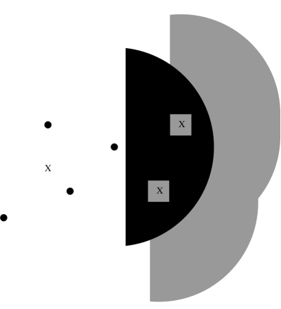
Figure 1: The dots are the points of $\sigma_{1}$, and the crosses are the points of $\sigma_{2}$. The grey squares are the set $\tilde{\sigma}_{2}^{+}$ (since $\varepsilon=\varepsilon_{n}<1/99$, they should really be smaller). Event $A_{\sigma}^{+}$ says that the black region contains no points of ${\cal Q}_{\tau\nu(n+1)}^{F}$ and the grey region (partly obscured by the black region) contains no points of ${\cal P}_{\nu(n+1)}^{F}$.

Suppose $k$ is such that $Q_{k}\cap B_{\sigma}^{+}\neq\emptyset$. Then by the triangle equality,

$$\|q_{k}-q_{j}\|\leq r_{\nu(n)}(1-5\varepsilon)+\varepsilon r_{\nu(n)}=r_{\nu(n)}(1-4\varepsilon).$$ (3.7)

Similarly, if $Q_{k}\cap B_{\sigma}^{-}\neq\emptyset$ then $\|q_{k}-q_{i}\|\leq r_{\nu(n)}(1-4\varepsilon)$.

By our coupling of Poisson processes, for $\nu(n)\leq n^{\prime}<\nu(n+1)$ we have ${\cal P}_{\nu(n)}\subset{\cal P}_{n^{\prime}}\subset{\cal P}_{\nu(n+1)}$. Also if $x\in Q_{k}$ and $y\in Q_{i}$ with $\|q_{i}-q_{k}\|\leq r_{\nu(n)}(1-3\varepsilon)$, then by the triangle inequality and our condition on $n_{1}$ we have $\|x-y\|\leq r_{\nu(n)}(1-\varepsilon)\leq r_{n^{\prime}}$ for all $n^{\prime}\in[\nu(n),\nu(n+1))$. Hence by the argument at $(\ref{0903a})$, for any $\sigma\in{\cal A}_{n,m}$ we have $E_{\sigma}\subset A_{\sigma}^{+}\cap A_{\sigma}^{-}$.

First we prove $(\ref{Ani2})$. Take $\sigma\in{\cal A}_{\nu(n),m}^{1}$. Consider just the case where $\sigma$ is near to the left edge of $[0,1]^{2}$ (the other three cases are treated similarly). If $\sigma_{2}^{+}=\emptyset$, then $A_{\sigma}^{+}=\{{\cal Q}_{\tau\nu(n+1)}^{F}(B^{+}_{\sigma})=0\}$, and in this case we have

$$\mathbb{P}[A_{\sigma}^{+}]\leq\exp(-\tau\nu(n)(\pi(r_{\nu(n)}(1-5\varepsilon))^{2}-2\varepsilon r_{\nu(n)}^{2})/2)$$

$$\leq\exp\left[-\tau\alpha(\log\nu(n))(1-12\varepsilon)/2\right]\leq\nu(n)^{-(1+\varepsilon)/2},$$ (3.8)

where the last inequality comes from $(\ref{epscond})$. This proves $(\ref{Ani2})$ for this case.

Suppose instead that $\sigma_{2}^{+}\neq\emptyset$. Then $\tilde{\sigma}_{2}^{+}\subset\{q_{j}\}\oplus B_{+}(r_{\nu(n)}(1-3\varepsilon))$ so that $v_{2}(\tilde{\sigma}_{2}^{+})\leq\pi r_{\nu(n)}^{2}(1-3\varepsilon)^{2}/2$. Let $s\in[0,1]$ be chosen such that $v_{2}(\tilde{\sigma}_{2}^{+})=s^{2}\pi r_{\nu(n)}^{2}(1-3\varepsilon)^{2}/2$. Then by the Brunn-Minkowski inequality (see e.g. [6]),

$$v_{2}(\tilde{\sigma}_{2}^{+}\oplus B_{+}(r_{\nu(n)}(1-3\varepsilon)))\geq(\pi r_{\nu(n)}^{2}/2)(1-3\varepsilon)^{2}(1+s)^{2},$$

and also $v_{2}(B_{\sigma}^{+})\geq\pi r_{\nu(n)}^{2}((1-5\varepsilon)^{2}-2\varepsilon)/2$ so that

$$\mathbb{P}[A_{\sigma}^{+}]\leq\exp(-\tau\nu(n)v_{2}(B_{\sigma}^{+}\setminus\tilde{\sigma}_{2}^{+})-\nu(n)v_{2}(\tilde{\sigma}_{2}^{+}\oplus B_{+}(r_{\nu(n)}(1-3\varepsilon))))$$

$$\leq\exp(-(\nu(n)\pi r_{\nu(n)}^{2}/2)[\tau((1-5\varepsilon)^{2}-2\varepsilon-s^{2}(1-3\varepsilon)^{2})+(1+s)^{2}(1-3\varepsilon)^{2}])$$

$$\leq\exp(-(\alpha/2)(\log\nu(n))g_{\tau}(s)),$$

where we set $g_{\tau}(s):=(\tau+1+2s)(1-12\varepsilon)+s^{2}(1-3\varepsilon)^{2}(1-\tau)$. If $\tau\leq 1$ then $g_{\tau}(s)$ is minimised over $s\in[0,1]$ at $s=0$. If $\tau>1$, then $g_{\tau}(\cdot)$ is concave, so its minimum over $[0,1]$ is achieved at $s=0$ or $s=1$; also in this case $g_{\tau}(1)\geq(3+\tau)(1-12\varepsilon)+1-\tau$. Hence, using $(\ref{epscond})$ and $(\ref{epscond2})$ we obtain

$$\mathbb{P}[A_{\sigma}^{+}]\leq\exp(-(\alpha/2)(\log\nu(n))\min[(1+\tau)(1-12\varepsilon),4-12\varepsilon(3+\tau)])$$

$$\leq\nu(n)^{-(1+\varepsilon)/2},$$ (3.9)

completing the proof of $(\ref{Ani2})$.

Now we prove $(\ref{Ani1})$. If $\sigma\in{\cal A}^{2}_{n,m}$ then $\mathbb{P}[A_{\sigma}^{+}]\leq\nu(n)^{-(1+\varepsilon)/2}$ by $(\ref{0903c})$ and $(\ref{0903b})$, and $\mathbb{P}[A_{\sigma}^{-}]\leq\nu(n)^{-(1+\varepsilon)/2}$ similarly. Therefore $\mathbb{P}[E_{\sigma}]\leq\mathbb{P}[A_{\sigma}^{+}\cap A_{\sigma}^{-}]\leq\nu(n)^{-1-\varepsilon},$ completing the proof of $(\ref{Ani1})$.

To prove $(\ref{Ani3})$, let $\sigma\in{\cal A}_{n,m}^{0}$. Assume $\sigma$ is near the lower left corner of $[0,1]^{2}$ (the other cases are treated similarly). First suppose $\sigma_{2}^{+}=\emptyset$. Then $\mathbb{P}[E_{\sigma}]\leq\mathbb{P}[{\cal Q}_{\tau\nu(n+1)}^{F}(B_{\sigma}^{+})=0]$ and since the upper half of $B_{\sigma}^{+}$ is contained in $[0,1]^{2}$, in this case

$$\mathbb{P}[E_{\sigma}]\leq\exp(-\tau\nu(n)\pi r_{\nu(n)}^{2}[((1-5\varepsilon)^{2}/4)-\varepsilon/2])$$

$$\leq\nu(n)^{-\alpha\tau(1-12\varepsilon)/4}\leq\nu(n)^{-(1+\varepsilon)/4}.$$ (3.10)

Now suppose $\sigma_{2}^{+}\neq\emptyset$. Let $q_{\ell}$ be the last element (in the lexicographic order) of $\sigma_{2}^{+}$. Then

$$\mathbb{P}[E_{\sigma}]\leq\mathbb{P}[{\cal P}_{\nu(n+1)}^{F}(\{q_{\ell}\}\oplus B_{+}(r_{\nu(n)}(1-3\varepsilon)))=0]$$

$$\leq\exp(-{\nu(n)}\pi r_{\nu(n)}^{2}(1-3\varepsilon)^{2}/4)\leq\nu(n)^{-\alpha(1-6\varepsilon)/4}\leq\nu(n)^{-1/20},$$

where for the last inequality we used the fact that $\alpha>1/4$ and $\varepsilon<1/99$. Together with $(\ref{0903d})$ this demonstrates $(\ref{Ani3})$.     

For $m,n\in\mathbb{N}$, and $r>0$, let ${\cal K}_{n,m}(r)$ be the class of bipartite point sets $({\cal X},{\cal Y})$ in $[0,1]^{2}$ such that $G({\cal X},{\cal Y},r)$ has at least one component, the vertex-set of which has projection onto ${\cal L}_{n}$ of order $m$ and contains at least one element of ${\cal X}$.

Lemma 3.6.

Let $m\in\mathbb{N}$. Then almost surely, for all but finitely many $n\in\mathbb{N}$ we have $({\cal P}_{n^{\prime}}^{F},{\cal Q}_{\tau{n^{\prime}}}^{F})\notin{\cal K}_{\nu(n),m}(r_{n^{\prime}})$ for all $n^{\prime}\in\mathbb{N}\cap[\nu(n),\nu(n+1))$.

Proof. By Lemmas 3.3 and 3.5, for $n\geq n_{1}$ we have

$$\mathbb{P}[\cup_{\nu(n)\leq n^{\prime}<\nu(n+1)}\{({\cal P}_{n}^{F},{\cal Q}_{\tau n}^{F})\in{\cal K}_{\nu(n),m}(r_{n^{\prime}})\}]\leq\sum_{\sigma\in{\cal A}_{\nu(n),m}}\mathbb{P}(E_{\sigma})$$

$$\leq|{\cal A}_{\nu(n),m}^{2}|\times\nu(n)^{-(1+\varepsilon)}+|{\cal A}_{\nu(n),m}^{1}|\times\nu(n)^{-(1+\varepsilon)/2}+|{\cal A}_{\nu(n),m}^{0}|\times\nu(n)^{-1/20}$$

and using Lemma 3.4 and the definition $\nu(n):=n^{\lceil 4/\varepsilon_{0}\rceil}$, and recalling that $\varepsilon=\varepsilon_{n}\geq\varepsilon_{0}$ as described just after (3.3), we find that this probability is $O(n^{-2})$, so is summable in $n$; then the result follows by the Borel-Cantelli lemma.     

Lemma 3.7.

(see [6, Lemma 9.1].) For any two closed connected subsets $A,B$ of $[0,1]^{2}$ with union $A\cup B=[0,1]^{2}$, the intersection $A\cap B$ is connected.

Given $n\in\mathbb{N}$, let $k(n)$ be the choice of $k\in\mathbb{N}$ satisfying $\nu(k)\leq n<\nu(k+1)$. Also, given $K\in\mathbb{N}$, let $F_{K}(n)$ be the event that $G({\cal P}_{n}^{F},{\cal Q}_{\tau n}^{F},r_{n})$ has two or more components with projections onto ${\cal L}_{\nu(k(n))}$ of order greater than $K$.

Lemma 3.8.

There exists $K\in\mathbb{N}$ such that with probability 1 the event $F_{K}(n)$ occurs for only finitely many $n$.

Proof. Suppose $F_{K}(n)$ occurs. Then there exist distinct components $U=(U_{1},U_{2})$, and $V=(V_{1},V_{2})$ in $G({\cal P}_{n}^{F},{\cal Q}^{F}_{\tau n},r_{n})$, both with projections onto ${\cal L}_{\nu(k(n))}$ of order greater than $K$. Let $U^{\prime}$ be the union of closed Voronoi cells in $[0,1]^{2}$ (relative to ${\cal P}_{n}\cup{\cal Q}_{\tau n}$) of vertices of $U$, and let $V^{\prime}$ be the union of closed Voronoi cells in $[0,1]^{2}$ of vertices of $V$.

The interior of $U^{\prime}$ and the interior of $V^{\prime}$ are disjoint subsets of $[0,1]^{2}$, and we now show that they are connected sets. Suppose $X\in U_{1},Y\in U_{2}$ with $\|X-Y\|\leq r_{n}$; then we claim the entire line segment $[X,Y]$ is contained in the interior of $U^{\prime}$. Indeed, let $z\in[X,Y]$, and suppose $z$ lies in the closed Voronoi cell of some $W\in{\cal P}_{n}^{F}\cup{\cal Q}_{\tau n}^{F}$. If $W\in{\cal P}_{n}^{F}$ then

$$\|W-Y\|\leq\|W-z\|+\|z-Y\|\leq\|X-z\|+\|z-Y\|=\|X-Y\|\leq r_{n}$$

so $W\in U$. Similarly, if $W\in{\cal Q}_{\tau n}^{F}$ then $\|W-X\|\leq r_{n}$ so again $W\in U$. Hence the interior of $U^{\prime}$ is connected, and likewise for $V^{\prime}$.

Let $\tilde{V}$ be the closure of the component of $[0,1]^{2}\setminus U^{\prime}$, containing the interior of $V^{\prime}$, and let $\tilde{U}$ be the closure of $[0,1]^{2}\setminus\tilde{V}$ (essentially, this is the set obtained by filling in the holes of $U^{\prime}$ that are not connected to $V^{\prime}$).

Then $\tilde{U},\tilde{V}$ are closed connected sets, whose union is $[0,1]^{2}$. Therefore by Lemma 3.7, the set $\partial U:=\tilde{U}\cap\tilde{V}$ is connected. Note that $\partial U$ is part of the boundary of $U^{\prime}$ (it is the ‘exterior boundary’ of $U^{\prime}$ relative to $V^{\prime}$).

Let $T$ be the set of cube centres $q_{i}\in{\cal L}_{\nu(k(n))}$ such that $Q_{i}\cap(\partial U)\neq\emptyset$. Then $T$ is $*$-connected in ${\cal L}_{\nu(k(n))}$, i.e. for any $x,y\in T$, there is a path $(x_{0},x_{1},\ldots,x_{k})$ with $x_{0}=x$, $x_{k}=y$ and $x_{i}\in{\cal L}_{\nu(k(n))}$ and $\|x_{i}-x_{i-1}\|_{\infty}=\varepsilon r_{\nu(k(n))}$ for $1\leq i\leq k$ (here $\varepsilon=\varepsilon_{\nu(k(n))}$.)

Also, for each $q_{i}\in T$ we claim ${\cal P}_{n}(Q_{i}){\cal Q}_{\tau n}(Q_{i})=0$. Indeed, suppose on the contrary that ${\cal P}_{n}(Q_{i}){\cal Q}_{\tau n}(Q_{i})>0$. Then all points of $({\cal P}_{n}\cup{\cal Q}_{\tau n})\cap Q_{i}$ lie in the same component of $G({\cal P}_{n}^{F},{\cal Q}_{\tau n}^{F},r_{n})$. If they are all in $U$, then $Q_{i}$, and all neighbouring $Q_{j}$ (including diagonal neighbours) are contained in $U^{\prime}$. If all points of $({\cal P}_{n}\cup{\cal Q}_{\tau n})\cap Q_{i}$ are not in $U$, then $Q_{i}$, and all neighbouring $Q_{j}$ (including diagonal neighbours) are disjoint from $U^{\prime}$. Therefore $(\partial U)\cap Q_{i}=\emptyset$.

We now prove the isoperimetric inequality

$$|T|\geq(K/2)^{1/2}.$$ (3.11)

To see this, define the width of a nonempty closed set $A\subset[0,1]^{2}$ to be the maximum difference between $x$-coordinates of points in $A$, and the height of $A$ to be the maximum difference between $y$-coordinates of points in $A$.

We claim that either the height or the width of $\partial U$ is at least $(K/2)^{1/2}\varepsilon r_{\nu(k(n))}$. Indeed, if not, then $\partial U$ is contained in some square of side $(K/2)^{1/2}\varepsilon r_{\nu(k(n))}$, and then either $U^{\prime}$ or $V^{\prime}$ is contained in that square, so either $U$ or $V$ is contained in that square, contradicting the assumption that the projections of $U$ and of $V$ onto ${\cal L}_{\nu(k(n))}$ have order greater than $K$. For example, if the projection of $U$ has order greater than $K$, then at least one of $U_{1}$ and $U_{2}$, say $U_{1}$, has projection of order greater than $K/2$, and then the union of squares of side $\varepsilon r_{\nu(k(n))}$ centred at vertices in the projection of $U_{1}$ has total area greater than $(K/2)\varepsilon^{2}r_{\nu(k(n))}^{2}$, so is not contained in any square of side $(K/2)^{1/2}\varepsilon r_{\nu(k(n))}$. Thus the claim holds, and then $(\ref{isoperi})$ follows by the $*$-connectivity of $T$.

For $\nu,m\in\mathbb{N}$, let ${\cal A}^{\prime}_{\nu,m}$ be the set of $*$-connected subsets of ${\cal L}_{\nu}$ with $m$ elements. By a similar argument to the proof of Lemma 3.4 (see also [6, Lemma 9.3]), there are finite constants $\gamma$ and $C$ such that for all $\nu,m\in\mathbb{N}$ we have

$$|{\cal A}^{\prime}_{\nu,m}|\leq C(\nu/\log\nu)\gamma^{m}.$$ (3.12)

Set $\phi_{n}:=\mathbb{P}[{\cal P}_{n}(Q_{i}){\cal Q}_{\tau n}(Q_{i})=0]$ (which does not depend on $i$). By the union bound, and $(\ref{0818a})$,

$$\phi_{n}\leq\exp(-n(\varepsilon r_{\nu(k(n))})^{2})+\exp(-\tau n(\varepsilon r_{\nu(k(n))})^{2})$$

$$\leq 2\exp[-(\tau\wedge 1)\varepsilon^{2}(\alpha/\pi)(n\log\nu(k(n))/\nu(k(n)))]$$

$$\leq 2\nu(k(n))^{-(\tau\wedge 1)\varepsilon^{2}\alpha/\pi}\leq 3n^{-(\tau\wedge 1)\varepsilon^{2}\alpha/\pi},$$

where the last inequality holds for all large enough $n$. Using $(\ref{isoperi})$ and $(\ref{0903e})$ we obtain that

$$\mathbb{P}[F_{K}(n)]\leq\sum_{m\geq(K/2)^{1/2}}C(\nu(k(n))/\log\nu(k(n)))\gamma^{m}\phi_{n}^{m}$$

$$\leq 2Cn(3\gamma n^{-\varepsilon^{2}\alpha(\tau\wedge 1)/\pi})^{(K/2)^{1/2}},$$

which is summable in $n$ provided $K$ is chosen so that $\varepsilon^{2}\pi^{-1}\alpha(\tau\wedge 1)(K/2)^{1/2}>3$. The result then follows by the Borel-Cantelli lemma.     

Proof of Theorem 3.1. Choose $K\in\mathbb{N}$ as in Lemma 3.8. Writing ‘i.o.’ for ‘for infinitely many $n$’ (i.e. infinitely often), we have

$$\mathbb{P}[{\cal G}^{1}(n,\tau,r_{n})\notin{\cal K}\mbox{ i.o.}]\leq\left(\sum_{m=1}^{K}\mathbb{P}[({\cal P}_{n}^{F},{\cal Q}_{\tau n}^{F})\in{\cal K}_{\nu(k(n)),m}(r_{n})\mbox{ i.o.}]\right)+\mathbb{P}[F_{K}(n)\mbox{ i.o.}].$$

By Lemmas 3.6 and 3.8, this is zero.