Experimental evaluation of the nuclear neutron-proton contact

Abstract

The nuclear neutron-proton contact is introduced, generalizing Tan’s work, and evaluated from medium energy nuclear photodisintegration experiments. To this end we reformulate the quasi-deuteron model of nuclear photodisintegration and establish the bridge between the Levinger constant and the contact. Using experimental evaluations of Levinger’s constant we extract the value of the neutron-proton contact in finite nuclei and in symmetric nuclear matter. Assuming isospin symmetry we propose to evaluate the neutron-neutron contact through measurement of photonuclear spin correlated neutron-proton pairs.

Introduction – Considering a system of two-component fermions interacting via a short range interaction, Tan Tan08 ; Bra12 has established a series of relations between the amplitude of the high-momentum tail of the momentum distribution $n_{\sigma}(k)$, where $\sigma$ is the spin, and the properties of the system, such as the energy, pair correlations and pressure. These relations, commonly known as the “Tan relations”, are expressed through a new variable the “Contact” $C=\lim_{k\rightarrow\infty}k^{4}n_{\sigma}(k)$. The contact, being a state variable depends on the density of the system (usually expressed through the Fermi momentum $k_{F}$), its temperature, composition, and its thermodynamic state. The Tan relations are universal, they hold for few-body as well as for many-body systems, for ground state and for finite temperature, for normal state but also for superfluid state. Their validity range depends on the interparticle distance $d\propto 1/k_{F}$ and the magnitude of the scattering length being both much larger than the potential range, usually characterized by the effective range $r_{\mathrm{eff}}$.

The theoretical discovery of the Tan relations has led to a concentrated experimental effort to measure and verify them in ultracold atomic systems, where the scattering length as well as the density can be controlled. These efforts have led to experimental verification of Tan’s relations in fermionic ⁴⁰K SteGaeDra10 ; SagDraPau12 and ⁶Li ParStrKam05 ; WerTarCas09 ; KuhHuLiu10 systems. It was also found that the measured value of the contact, as function of $(k_{F}a)^{-1}$ along the BCS-BEC crossover, is in accordance with the theoretical predictions of WerTarCas09 .

In this manuscript we focus on nuclear systems. Generalizing Tan’s work, we introduce the nuclear contacts and present an experimental evaluation of the neutron-proton contact in finite nuclei and also in symmetric nuclear matter. To this end we relate the contact to medium energy photonuclear cross-section and utilize available experimental data. In ultracold atomic physics the ratio between the interparticle distance $1/k_{F}$, the scattering length $a$, and $r_{\mathrm{eff}}$ can be controlled in such a way as to ensure that the $a\gg r_{\mathrm{eff}}$ and $k_{F}r_{\mathrm{eff}}\ll 1$. The nuclear two–body scattering length is about 5.38 fm when the two nucleons are in the ${}^{3}S_{1}$ state and about -20 fm when they are in the ${}^{1}S_{0}$ state. These scattering lengths are denoted by $a_{t}$ for the ${}^{3}S_{1}$ channel, and $a_{s}$ for the ${}^{1}S_{0}$ channel. The average interparticle distance in the atomic nucleus is about $2.4\;\mathrm{fm}$. This number can be deduced from the empirical nuclear charged radius formula $R_{c}\approx 1.2A^{1/3}\;\mathrm{fm}$. The long range part of the nuclear potential is governed by the pion exchange Yukawa force with characteristic length of $\mu^{-1}=\hbar/m_{\pi}c\approx 1.4\;\mathrm{fm}$. Therefore in contrast with atomic physics, in nuclear physics the demand $k_{F}r_{\mathrm{eff}}\ll 1$ can at best replaced by $\mu d>1$ which holds for interparticle distance of about 2 fm.

For photons in the energy range $\hbar\omega=100-200\;\mathrm{MeV}$, corresponding to the wave number $k\approx 0.5-1\;\mathrm{fm}^{-1}$, the deuteron photoabsorption cross-section is dominated by the leading electric dipole $E1$ and magnetic dipole $M1$ transitions Arenhovel91 . The nuclear photo effect at these energies is dominated by the quasi-deuteron process first proposed by Levinger more than 60 years ago Lev51 . In the quasi-deuteron picture the photonuclear reaction mechanism goes through an absorption of the photon by a correlated proton-neutron ($pn$) pair being close to each other, followed by an emission of the $pn$ pair back to back, flying without further interaction with the remaining nucleons. The resulting photonuclear cross-section of a nucleus composed of $Z$ protons and $N$ neutrons, $A=N+Z$, is therefore proportional to the deuteron cross-section $\sigma_{d}$,

$$\sigma_{A}=L\frac{NZ}{A}\sigma_{d}$$ (1)

with $L\approx 6$ being the Levinger constant. In the decades following Levinger’s original work there were few compilations of the photonuclear data and systematic evaluations of the Levinger constant (see e.g. TavTer92 and references therein). It was also found that 2–body short range correlations captured so well by the quasi-deuteron model plays an important role in analyzing hard nuclear electron scattering experiments, see e.g. LO90 ; FS88 ; WirSchPie14 . Moreover, Levinger’s picture has got a remarkable experimental support when high momentum, correlated, $pn$ pairs flying back to back where measured in proton and electron scattering on carbon Piasetzky06 ; Subedi08 and other nuclei ArrHigRos12 ; Fom12 .

Already from the pictorial description of the quasi-deuteron model one can sense the underlying connection between Tan’s contact and Levinger’s constant. In the following we shall define the various nuclear contacts associated with the permissible two-nucleon $s$-wave states. Utilizing these contacts we shall rederive the quasi-deuteron model, establishing the desired connection. As will be evident later, the nuclear contacts can be evaluated from either spin independent transitions or from experiments on spherical nuclei. Consequently we shall concentrate on the $E1$ transition cross-section, which in principle can be extracted from the angular distribution of the emitted $pn$ pair. The experimental evaluation of Levinger’s constant TavTer92 is than used to extract the proton-neutron contact.

The Contact in Nuclear Systems – When two particles interacting via short range force approach each other, the many-body wave function can be factorized into a product of an asymptotic pair wave function $\varphi_{ij}(\bm{r}_{ij})$, where $\bm{r}_{ij}=\bm{r}_{i}-\bm{r}_{j}$, and a function $A_{ij}$, also called the regular part of $\Psi$, describing the residual $A-2$ particle system and the pair’s center of mass (CM) $\bm{R}_{ij}=(\bm{r}_{i}+\bm{r}_{j})/2$ motion Tan08 ; WerCas12 ,

$$\Psi\xrightarrow[r_{ij}\rightarrow 0]{}\varphi_{ij}(\bm{r}_{ij})A_{ij}(\bm{R}_{ij},\{\bm{r}_{k}\}_{k\neq i,j})\;.$$ (2)

Due to the suppression of higher partial waves, the pair wave function will be predominantly an $s$-wave. In particular, in the zero-range model zerorange , where the action of an interacting particle pair with scattering length $a$ on the many-body wave-function $\Psi$ is represented through the boundary condition $\left[{\partial\log(r_{ij}\Psi)}/{\partial r_{ij}}\right]_{r_{ij}=0}=-{1}/{a}$ , the low energy asymptotic pair wave function takes a particularly simple form $\varphi_{ij}=\left(1/r_{ij}-1/a\right)$.

The contact $C$ represents the probability of finding a correlated pair within the system, and can be expressed as Tan08 ; WerCas12

$$C=16\pi^{2}\sum_{i<j}\langle A_{ij}|A_{ij}\rangle$$ (3)

where

$$\langle A_{ij}|A_{ij}\rangle =\int\prod_{k\neq i,j}d\bm{r}_{k}\,d\bm{R}_{ij}\,$$ (4)

$$\times A_{ij}^{\dagger}\left(\bm{R}_{ij},\{\bm{r}_{k}\}_{k\neq i,j}\right)\cdot A_{ij}\left(\bm{R}_{ij},\{\bm{r}_{k}\}_{k\neq i,j}\right)\;$$

is independent of the particular form of the asymptotic pair wave function $\varphi_{ij}$. The Pauli principle implies that $A_{ij}=0$ if the two particles are in the same internal state.

Generalizing this formalism to nuclear systems, the pair can be in more than one configuration, and we have to consider six possible pairs $P=\{p\!\uparrow\!p\!\downarrow,n\!\uparrow\!n\!\downarrow,p\!\uparrow\!n\!\downarrow,p\!\uparrow\!n\!\uparrow,p\!\downarrow\!n\!\uparrow,p\!\downarrow\!n\!\downarrow\}$. In this representation we can define a contact $C_{P}$ for each pair $P$. These contacts are proportional to the diagonal elements of the overlap matrix $\langle A_{ij}^{P}|A_{ij}^{P^{\prime}}\rangle$. In nuclear physics it is more natural, however, to employ a spin-isospin basis that diagonalize the overlap matrix. Furthermore, assuming now spin symmetry for the residual function norm $\langle A_{ij}^{P}|A_{ij}^{P}\rangle$ we have to consider only four contacts associated with the pairs $P=\{(pp)_{S=0},(nn)_{S=0},(np)_{S=0},(np)_{S=1}\}$. Taking into account that the coulomb force as well as other isospin symmetry-breaking terms are negligible at short distances, the number of independent nuclear contacts in symmetric nuclei $(N=Z)$ can be further reduced to only two, corresponding to the two-body spin-isospin configurations $\{|S=0,T=1\rangle,|S=1,T=0\rangle\}$. In the quasi-deuteron mechanism described above only correlated $pn$ pairs play any role, thus we need to consider only the two nuclear contacts $\{C_{s},C_{t}\}$ corresponding to the spin singlet and spin triplet states.

In bosonic systems the high momentum tail of the momentum distribution contains a $1/k^{5}$ correction due to three body contact BraKanPla11 . We note that such correction is to be expected in nuclear systems, as three nucleon coalescence is not forbidden by the Pauli exclusion principle. Studying 3-body effects on the nuclear photoabsorption cross-section and consequently estimating the nuclear 3-body contact is an important task. Nevertheless in the current letter we focus on the leading 2-body effect.

The Quasi-Deuteron model in the zero range approximation – In the following we will utilize the zero range approximation to relate the contact to the quasi-deutron model. This model allows a clear and simple derivation. We note however, that it can be easily generalized to include more realistic wave functions.

In the leading $E1$ approximation, the total photo absorption cross section of a nucleus is given by

$$\sigma_{A}(\omega)=4\pi^{2}\alpha\hbar\omega R(\omega)\,,$$ (5)

where $\alpha$ is the fine structure constant,

$$R(\omega)=\bar{\sum_{i}}\sum_{f}\left|\langle\Psi_{f}\right|\bm{\epsilon}\cdot\hat{\bm{D}}\left|\Psi_{0}\rangle\right|^{2}\delta(E_{f}-E_{0}-\hbar\omega)$$ (6)

is the response function, $\hat{\bm{D}}$ is the unretarded dipole operator $\hat{\bm{D}}=\sum_{i=1}^{A}\frac{1+\tau^{3}_{i}}{2}\bm{r}_{i}$, and ${\bm{\epsilon}}$ is the photon’s polarization vector. The wave functions of the initial (ground) state and of the final state are denoted by $\left|\Psi_{0/f}\right\rangle$ and the energies by $E_{0/f}$, respectively. The operator $\tau^{3}_{i}$ is the third components of the $i$-th nucleon isospin operator. The response functions includes a sum over the final states $\sum_{f}$ that becomes an integration in the limit of infinite volume, and an average over the initial states which amounts to an average over the magnetic projection of the ground state, $\bar{\sum}_{i}=1/(2J_{0}+1)\sum_{M_{0}}$.

For inverse photon wave number somewhat shorter than the average interparticle distance ($kd>1$), the reaction cross-section goes via a nucleon pair that absorbs the photon. The $E1$ nature of the process implies that the pair must be a neutron-proton pair since proton-proton pair posses no dipole moment. Utilizing the zero-range approximation,

$$\Psi_{0}\xrightarrow[r_{pn}\rightarrow 0]{} \sum_{P}\left(\frac{1}{r_{pn}}-\frac{1}{a_{P}}\right)A^{P}_{pn}\left(\bm{R}_{pn},\{\bm{r}_{j}\}_{j\neq p,n}\right)$$ (7)

$$+O(r_{pn}),$$ (8)

where $A^{P}_{pn}=\sum_{J_{A-2}}\left[\chi_{P}\otimes A_{P}^{J_{A-2}}(\bm{R}_{pn},\{\bm{r}_{j}\}_{j\neq p,n})\right]^{J_{0}M_{0}}.$ Here the notation $pn$ stands for any proton-neutron pair, whose spinors are coupled into a spin state $\chi_{P}$ with total spin $S=0,1$, and the corresponding scattering length $a_{P}$. The sum over the angular momentum of the remaining $A-2$ nucleons $J_{A-2}$ extends over all possible configurations that coupled to $S$ yield the ground state’s total angular momentum quantum numbers $J_{0},M_{0}$.

Turning now to the final state, we consider a reaction mechanism where the photon is absorbed by a proton $p$ that is emitted with large momentum $\mathbf{k}_{p}$. For high photon energies this process is fast enough and interaction between the emitted proton and rest of the nucleus can be neglected, that is the Born approximation. Hence, momentum conservation implies that another particle must be emitted. As pointed out by Levinger Lev51 , this particle must be a neutron $n$ emitted with momentum $\mathbf{k}_{n}$, such as $\mathbf{k}_{n}\approx-\mathbf{k}_{p}\equiv\mathbf{k}$. The relative momentum of the emitted particles is $\frac{\mathbf{k}_{n}-\mathbf{k}_{p}}{2}=\frac{2\mathbf{k}_{n}}{2}=\mathbf{k}$, and they can form either an $S=0$ or an $S=1$ spin states. Assuming that the residual $A-2$ particles wave function is frozen throughout this process, the final state wave function for an outgoing spin $S$ pair is given by

$$\Psi_{f}^{P}={\cal N}_{P}\hat{\cal A}\left\{\frac{1}{\sqrt{\Omega}}e^{-i\mathbf{k}\cdot\mathbf{r}_{pn}}A^{P}_{pn}(\bm{R}_{pn},\{\bm{r}_{j}\}_{j\neq p,n})\right\}\;,$$ (9)

where ${\cal N}_{P}$ is a normalization factor, the wave function is normalized in a box of volume $\Omega$, and $\hat{\cal A}=\big{(}1-\sum_{p^{\prime}\neq p}(p,p^{\prime})\big{)}\big{(}1-\sum_{n^{\prime}\neq n}(n,n^{\prime})\big{)}$ is the proton-neutron antisymmetrization operator with $(i,j)$ the transposition operator. The sums over $p^{\prime},n^{\prime}$ extends over all protons and neutrons in the system but $p,n$. As $A^{P}_{pn}(\bm{R}_{pn},\{\bm{r}_{j}\}_{j\neq p,n})$ is antisymmetric under permutation of all identical particles but the pair $pn$, $\Psi_{f}^{P}$ is antisymmetric under proton permutations and under neutron permutations.

Utilizing now permutational symmetry, the nuclear neutron-proton contacts $C_{P}=\{C_{s},C_{t}\}$ are given by

$$C_{P}=16\pi^{2}NZ\langle A^{P}_{pn}|A^{P}_{pn}\rangle\;.$$ (10)

Therefore, the normalization factor is given by ${\cal N}_{P}=\frac{1}{\sqrt{NZ}}\frac{1}{\sqrt{\langle A^{P}_{pn}|A^{P}_{pn}\rangle}}=\frac{4\pi}{\sqrt{C_{P}}}$. Considering now the transition matrix element we see that

$$\langle\Psi_{f}^{P}| \bm{\epsilon}\cdot\hat{\bm{D}}|\Psi_{0}\rangle=NZ{\cal N}_{P}\int\prod_{k}d\bm{r}_{k}$$ (11)

$$\times\frac{1}{\sqrt{\Omega}}e^{i\mathbf{k}\cdot\mathbf{r}_{pn}}A_{pn}^{P\dagger}\left(\mathbf{R}_{pn},\{\mathbf{r}_{j}\}_{j\neq pn}\right)\left(\bm{\epsilon}\cdot\hat{\bm{D}}\right)\Psi_{0}$$

where we have used the fact that $\hat{\cal A}\Psi_{0}=NZ\Psi_{0}$. Due to the orthogonality of the initial and final states the transition matrix element vanishes unless the photon acts on the outgoing $pn$ pair. Since the momentum $\mathbf{k}$ is large, the only significant contribution to the integral comes from the asymptotic $r_{pn}\rightarrow 0$, where $\Psi_{0}$ diverges, and therefore the integration over $r_{pn}$ hereafter can be limited to a small neighborhood of the origin $\Omega_{0}$. See Supplemental Material supplemental for more details. Hence,

$$\langle\Psi_{f}^{P}| \bm{\epsilon}\cdot\hat{\bm{D}}|\Psi_{0}\rangle=NZ{\cal N}_{P}\sum_{P^{\prime}}\langle A^{P}_{pn}|A^{P^{\prime}}_{pn}\rangle$$ (12)

$$\times\int_{\Omega_{0}}d\bm{r}_{pn}\frac{1}{\sqrt{\Omega}}e^{i\mathbf{k}\cdot\mathbf{r}_{pn}}\left(\bm{\epsilon}\cdot\hat{\bm{D}}_{pn}\right)\left(\frac{1}{r_{pn}}-\frac{1}{a_{P^{\prime}}}\right),$$

where $\hat{\bm{D}}_{pn}=\mathbf{r}_{p}\simeq\frac{\mathbf{r}_{pn}}{2}$ neglecting the pair’s CM motion. Most of the photon energy is delivered to the relative motion whereas the photon’s momentum is translated into the CM motion, thus the energy fraction associated with the CM coordinate $\bm{R}_{pn}$ is $\hbar\omega/4Mc^{2}$ which amounts to only few percents for the photon energies under consideration. We can therefore safely neglect the pair’s recoil. We note that the matrix element (12) is independent of $M_{0}$ thus $\bar{\sum}_{i}=1$ in Eq. (6). For the $E1$ operator or for any spin scalar operator the orthogonality of the different two-body spin functions included in $A_{P}$ ensures that the spin state of the $pn$ pair is unaltered throughout the process, i.e. $P^{\prime}=P$. For spherical $J_{0}=0$ nuclei this important result holds for any one-body nuclear current operator since the different singlet and triplet spin states must be coupled to spectator functions $A_{P}^{J_{A-2}}$ with $J_{A-2}=0,1$ respectively. These spectator functions are orthogonal and therefore there is no interference between the different $pn$ spin states. Utilizing these results we can rewrite the transition matrix element in the form

$$\langle\Psi_{f}^{P}|\bm{\epsilon} \cdot\hat{\bm{D}}|\Psi_{0}\rangle=$$ (13)

$$\frac{\sqrt{C_{P}}}{4\pi}\int_{\Omega_{0}}d\bm{r}_{pn}\frac{1}{\sqrt{\Omega}}e^{i\mathbf{k}\cdot\mathbf{r}_{pn}}\bm{\epsilon}\cdot\hat{\bm{D}}_{pn}\left(\frac{1}{r_{pn}}-\frac{1}{a_{P}}\right)\;.$$

The matrix element (13) looks very much as the deuteron’s photoabsorption transition matrix element. To make this comparison complete, let us consider the deuteron’s photoabsorption reaction. The deuteron is a bound proton-neutron pair with angular momentum $J=1$. In the zero range approximation, the deuteron wave function is assumed to be a pure $s$-wave, spin triplet state, that takes the form

$$\psi_{d,0}=\frac{1}{\sqrt{2\pi a_{t}}}\frac{e^{-r_{pn}/a_{t}}}{r_{pn}}\xrightarrow[r_{pn}\rightarrow 0]{}\frac{1}{\sqrt{2\pi a_{t}}}\left(\frac{1}{r_{pn}}-\frac{1}{a_{t}}\right).$$ (14)

In the Born approximation, and neglecting the CM recoil, the deuteron’s final state wave function is given by

$$\psi_{d,f}=\frac{1}{\sqrt{\Omega}}e^{-i\mathbf{k}\cdot\mathbf{r}_{pn}}.$$ (15)

Hence,

$$\langle\psi_{d,f}| \bm{\epsilon}\cdot\hat{\bm{D}}|\psi_{d,0}\rangle=$$ (16)

$$\int d\bm{r}_{pn}\frac{1}{\sqrt{\Omega}}e^{i\mathbf{k}\cdot\mathbf{r}_{pn}}\bm{\epsilon}\cdot\hat{\bm{D}}_{pn}\frac{1}{\sqrt{2\pi a_{t}}}\frac{e^{-r_{pn}/a_{t}}}{r_{pn}}.$$

Analyzing Eqs. (13) and (16) we note that in the high momentum limit $\bm{k}\longrightarrow\infty$ the main contribution to the transition matrix-element emerge from $\Omega_{0}$ the neighborhood of the origin $r_{pn}=0$. There, the $np$ pair wave function takes the asymptotic form $\left(1/{r_{pn}}-{1}/{a_{t}}\right)\approx 1/r_{pn}$. Utilizing this approximation and comparing Eqs. (13) and (16) we can conclude that

$$\langle\Psi_{f}^{P}|\bm{\epsilon}\cdot\hat{\bm{D}}|\Psi_{0}\rangle\approx\sqrt{\frac{C_{P}a_{t}}{8\pi}}\langle\psi_{d,f}|\bm{\epsilon}\cdot\hat{\bm{D}}|\psi_{d,0}\rangle$$ (17)

Substituting this result into Eq. (5) and summing over the possible final state spin configurations we get

$$\sigma_{A}(\omega)=\frac{a_{t}}{8\pi}(C_{s}+C_{t})\sigma_{d}(\omega)$$ (18)

where $\sigma_{d}(\omega)$ is the deuteron photonuclear cross-section. Comparing this result with the celebrated Levinger formula, Eq. (1), we see that the Levinger constant $L$ can be directly expressed through the nuclear contacts $C_{P}$,

$$L=\frac{a_{t}}{8\pi}\frac{A}{NZ}(C_{s}+C_{t})\;.$$ (19)

The Levinger constant was explored and evaluated in various photonuclear experiments. Using this data the averaged nuclear $pn$ contact $\bar{C}_{pn}\equiv(C_{s}+C_{t})/2$ can be evaluated.

Before we proceed to actual evaluation of the nuclear contact few comments are in place: (i) In our derivation we have utilized the zero range approximation. The validity of this approximation is at best questionable for finite nuclei. Nonetheless, the derivation can be generalized to any short range pair wave function given that it is unique across the nuclear chart. In this case, the resulting many-body contact should be expressed in terms of the deuteron contact, i.e. $8\pi/a_{t}$ is to be replaced by the deutron contact in Eqs. (18) and (19). (ii) Although we have only considered the dipole response, our main result (18) holds in spherical $J_{0}=0$ nuclei for any multipole and any one-body current operator. For $J_{0}\neq 0$ nuclei, Eq. (18) holds for any spin independent one-body operator. (iii) If instead of measuring the total photoabsorption cross-section one measures the cross-section $\sigma_{A}^{\uparrow\!\uparrow}$ for the parallel spin reaction $\gamma+^{A}\!X\longrightarrow^{A-2}\!Y+p\!\uparrow\!n\!\uparrow$, we would obtain

$$\sigma_{A}^{\uparrow\!\uparrow}(\omega)=\frac{1}{3}\frac{a_{t}}{8\pi}C_{t}\sigma_{d}(\omega)$$ (20)

for spherical $J_{0}=0$ nuclei. Thus, measuring the spin correlated photonuclear cross-section would enable the separation of the two nuclear contacts $C_{s}$ and $C_{t}$.

Experimental evaluation of the nuclear neutron-proton contact – At this point we would like to extract the nuclear neutron-proton contact from the experimental photonuclear data. To this end we use an analysis of the Levinger constant made by Terranova et al. TavTer92 , who evaluated the Levinger constant $L$ for 14 nuclei along the periodic table, from lithium to uranium, using various photonuclear experiments AhrBorCzo75 ; Sti84 ; Lep78 ; Hom83 . In order to include low energy data Terranova et al. have used in their analysis the modified quasi-deuteron model MQD , taking into account the Pauli blocking. For high photon energies this is a small correction. The evaluated Levinger constant, presented in Fig. 1, seems to be constant along the nuclear chart, with an averaged value of $L\approx 5.50\pm 0.21\;(1\sigma)$. Using this result we can estimate the average $pn$ contact for symmetric nuclei and nuclear matter, namely

$$\frac{\bar{C}_{pn}}{k_{F}A}=\frac{\pi}{k_{F}a_{t}}\left(5.50\pm 0.21\right)\approx 2.55\pm 0.10\;.$$ (21)

Here in the last equality we have used the relation $1/k_{F}a_{t}\approx 0.15$ valid on the average for large nuclei. We note that the quoted error in Eq. (21) refers only to statistical errors, and not to systematic errors associated with our model assumptions.

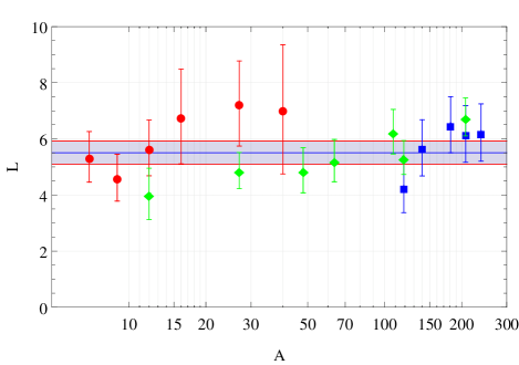
Figure 1: (Color online) Levinger constant values evaluated from photonuclear experiments. Red circles are based on Ref. AhrBorCzo75 , blue squares are based on Ref. Lep78 , and green diamonds are based on Ref. Sti84 . Adapted with changes from TavTer92 . The blue line shows the averaged value $L=5.50$, and the gray band its error.

As mentioned above, the contact was measured for a universal Fermi gas along the BCS-BEC crossover, i.e. as a function of the dimensionless parameter $k_{F}a$. In order to compare the nuclear $pn$ contact to the universal Fermi gas results we estimated $k_{F}$ for each nuclei using the rms charge radius, evaluated by Brown et al. BroBroHod84 . In Fig. 2 we present the universal Fermi gas contact measured with ⁴⁰K atoms SteGaeDra10 , and ⁶Li atoms ParStrKam05 ; WerTarCas09 , the theoretical prediction of Ref. WerTarCas09 , and the average nuclear $pn$ contact evaluated for each nucleus individually. For the nuclear scattering length we have used $1/a=1/2(1/a_{s}+1/a_{t})$, with error bar that corresponds to the difference between the singlet and triplet scattering lengths. Inspecting the figure it is noteworthy that although nuclei are far from being a universal Fermi gas, the nuclear contact falls in line with that of a universal Fermi gas.

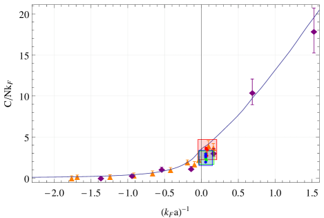
Figure 2: (Color online) The universal contact per particle (in units of $k_{F}$), measured in ultracold atoms, compared to the averaged $pn$ contact evaluated here from photonuclear experiments. Orange triangles - measurement with ultracold ⁴⁰K atoms SteGaeDra10 , purple diamonds - ultracold ⁶Li atoms ParStrKam05 ; WerTarCas09 . Red, blue and green dots - nuclear contact based on photonuclear experiments of AhrBorCzo75 , Lep78 , and Sti84 . The square’s bounds represent the experimental error for the different data sets. The line is the theoretical prediction of Ref. WerTarCas09 .

Summary – Summing up, rederiving the quasi-deuteron model in the zero range approximation we have constructed a bridge between the contact $C$, recently introduced by Tan to describe the properties of interacting Fermi systems, and nuclear systems. Doing so we have identified two contacts $C_{s},\;C_{t}$, corresponding to spin singlet and spin triplet states, and have shown that the average $pn$ contact $\bar{C}_{pn}$ is proportional to Levinger’s constant $L$. Using experimental estimates for $L$ we have deduced the value of $\bar{C}_{pn}$. We have found that the evaluated value of $\bar{C}_{pn}$ stands in good agreement with the universal contact measured in ultracold atomic experiments. This result hints towards the usefulness of Tan’s relations also in nuclear physics. To separate between the singlet and triplet contacts we propose to measure the spin correlated emitted pairs in photonuclear experiment.

Supplemental Materials: Experimental evaluation of the nuclear neutron-proton contact

In our letter we have argued that in the large k limit the photodisintegration matrix element is sensitive only to the most diverging part of the wave function, namely its behavior in short interparticle distances, and therefore we limit our integrals, for example Eq. (11), to a small neighborhood of the origin $\Omega_{0}$. Here we present in details the calculation of such integrals.

In the zero range approximation, the deuteron’s photodisintegration cross section is proportional to the integral

$$\int d\bm{r}e^{i\bm{k}\cdot\bm{r}}\bm{\epsilon}\cdot\bm{r}\frac{e^{-r/a}}{r}.$$ (S1)

For $k\longrightarrow\infty$, the main contribution to this integral comes from the neighborhood of the origin $r=0$, because the fast-oscillating $e^{i\mathbf{k}\cdot\mathbf{r}}$ washes out anything but the most diverging part of the function. In this neighborhood $e^{-r/a}\approx 1$, and the integral can be approximated by

$$\int_{\Omega_{0}}d\bm{r}e^{i\bm{k}\cdot\bm{r}}\bm{\epsilon}\cdot\bm{r}\frac{1}{r},$$ (S2)

where the integration is limited to a small neighborhood of the origin $\Omega_{0}$ by some smooth cutoff function $f_{R}(r)$,

$$\int_{\Omega_{0}}d\bm{r}g(r)\equiv\int d\bm{r}g(r)f_{R}(r),$$ (S3)

where $f_{R}(0)=1$.

First we note that similar approximation is used to prove the fundamental Tan relation Tan08 , namely

$$\lim_{k\rightarrow\infty}n_{\sigma}(k)=\frac{C}{k^{4}}.$$ (S4)

In the two body case ComAlzLey09 , one has to Fourier transform the dimer wave function,

$$\int d\bm{r}e^{i\bm{k}\cdot\bm{r}}\frac{e^{-r/a}}{r}=\frac{4\pi a^{2}}{a^{2}k^{2}+1}\xrightarrow[ka\gg 1]{}\frac{4\pi}{k^{2}}.$$ (S5)

To show that this integral is dominated, in the large k limit, by its short-range behavior, let’s approximate it by

$$\int_{\Omega_{0}}d\bm{r}e^{-i\bm{k}\cdot\bm{r}}\frac{1}{r}$$ (S6)

and use $f_{R}(r)=e^{-r/R}$ as a cutoff function. It is clear that the resulting integral is equivalent to (S5), and therefore reproduce the right limit. Using a Gaussian cutoff function $f_{R}(r)=e^{-(r/R)^{2}}$ one gets

$$\int d\bm{r}e^{i\bm{k}\cdot\bm{r}}\frac{1}{r}e^{-(r/R)^{2}}=\frac{4\pi R}{k}F\left(\frac{kR}{2}\right),$$ (S7)

where $F(x)=e^{-x^{2}}\int_{0}^{x}dye^{y^{2}}$ is the Dawson integral. For large $x$, $F(x)=(2x)^{-1}+(4x)^{-3}+O(x^{-4})$ and in the limit $kR\gg 1$ we obtain again $4\pi/k^{2}$. In fact, we may conclude that any smooth cutoff function such as $\exp(-r/R)$, $exp(-(r/R)^{2})$, or $(1-\tanh((r-R)/h))/(1+\tanh(R/h))$ will reproduce this result in the high momentum limit. In contrast, a sharp cutoff such as $f_{R}(r)=\Theta(R-r)$ will not work, because of the Gibbs phenomenon.

Note that here the same result can be achieved with $f_{R}(r)=1$, utilizing the relation $\Delta(1/r)=-4\pi\delta(\bm{r})$.

Now we go back to Eq. (S1) and show that the same approximation works there. First, operating with $\bm{\epsilon}\cdot\nabla_{k}$ on Eq. (S5), we get

$$\int d\bm{r}e^{i\bm{k}\cdot\bm{r}}\bm{\epsilon}\cdot\bm{r}\frac{e^{-r/a}}{r}=\frac{8\pi ia^{4}k}{\left(a^{2}k^{2}+1\right)^{2}}\bm{\epsilon}\cdot\hat{k}\xrightarrow[ka\gg 1]{}\frac{8\pi i\bm{\epsilon}\cdot\hat{k}}{k^{3}}.$$ (S8)

Once again a smooth cutoff function $f_{R}(r)=e^{-r/R}$ can be added to limit the integral in Eq. (S2) to a small neighborhood of the origin, yielding the same result for large $k$. We can also check the use of a Gaussian cutoff,

$$\int d\bm{r}e^{i\bm{k}\cdot\bm{r}}\bm{\epsilon}\cdot\bm{r}\frac{1}{r}e^{-(r/R)^{2}}=2\pi i\frac{R}{k^{2}}\bm{\epsilon}\cdot\hat{k}\left(-kR+\left((kR)^{2}+2\right)F\left(\frac{kR}{2}\right)\right)\xrightarrow[kR\gg 1]{}\frac{8\pi i\bm{\epsilon}\cdot\hat{k}}{k^{3}}.$$ (S9)

We may conclude that also in this case any smooth cutoff function will reproduce the right high momentum limit.

In conclusion, we have shown here that indeed for $k\longrightarrow\infty$ the main contribution to the integrals in Eqs. (S1) and (S5) comes from a small neighborhood of the origin. We have explained that it is important to limit the integrals by a smooth cutoff function, and we have checked it explicitly for exponential, Gaussian, and $\tanh$ cutoffs.

References

- (1) S. Tan, Ann. Phys. (N.Y.) 323, 2952 (2008); 323, 2971 (2008); 323, 2987 (2008).
- (2) R. Combescot, F. Alzetto,and X. Leyronas, Phys. Rev. A 79, 053640 (2009).