Lifted Variable Elimination for Probabilistic Logic Programming

Abstract

Lifted inference has been proposed for various probabilistic logical frameworks in order to compute the probability of queries in a time that depends on the size of the domains of the random variables rather than the number of instances. Even if various authors have underlined its importance for probabilistic logic programming (PLP), lifted inference has been applied up to now only to relational languages outside of logic programming. In this paper we adapt Generalized Counting First Order Variable Elimination (GC-FOVE) to the problem of computing the probability of queries to probabilistic logic programs under the distribution semantics. In particular, we extend the Prolog Factor Language (PFL) to include two new types of factors that are needed for representing ProbLog programs. These factors take into account the existing causal independence relationships among random variables and are managed by the extension to variable elimination proposed by Zhang and Poole for dealing with convergent variables and heterogeneous factors. Two new operators are added to GC-FOVE for treating heterogeneous factors. The resulting algorithm, called LP² for Lifted Probabilistic Logic Programming, has been implemented by modifying the PFL implementation of GC-FOVE and tested on three benchmarks for lifted inference. A comparison with PITA and ProbLog2 shows the potential of the approach.

1 Introduction

Over the last years, there has been increasing interest in models that combine first-order logic and probability, both for domain modeling under uncertainty, and for efficiently performing inference and learning [Getoor and Taskar (2007), De Raedt et al. (2008)]. Probabilistic Logic Programming (PLP) has recently received an increasing attention for its ability to incorporate probability in logic programming. Among the various proposals, the one based on the distribution semantics [Sato (1995)] has gained popularity as the basis of languages such as Probabilistic Horn Abduction [Poole (1993)], PRISM [Sato (1995)], Independent Choice Logic [Poole (1997)], Logic Programs with Annotated Disjunctions [Vennekens et al. (2004)], and ProbLog [De Raedt et al. (2007)].

Nonetheless, research in Probabilistic Logic Languages has made it very clear that it is crucial to design models that can support efficient inference, while preserving intensional, and declarative modeling. Lifted inference [Poole (2003), de Salvo Braz et al. (2005), Milch et al. (2008), Van den Broeck et al. (2011)] is one of the major advances in this respect. The idea is to take advantage of the regularities in structured models to decrease the number of operations. Originally, the idea was proposed as an extension of variable elimination (ve for short in the following). Work on lifting ve started with [Poole (2003)]. Lifted VE exploits the symmetries present in first-order probabilistic models, so that it can apply the same principles behind ve to solve a probabilistic query without grounding the model.

Most work in probabilistic inference compute statistics from a sum of products representation, where each element is named a factor. Lifted inference generates templates, named parametric factors or parfactors, which stand for a set of similar factors found in the inference process, thus delaying as much as possible the use of fully instantiated factors.

In [Gomes and Costa (2012)], the Prolog Factor Language (PFL, for short) was proposed as a Prolog extension to support probabilistic reasoning with parfactors. PFL exploits the state-of-art algorithm GC-FOVE [Taghipour et al. (2013)], which redefines the operations described in[Milch et al. (2008)] to be correct for whatever constraint representation is being used. This decoupling of the lifted inference algorithm from the constraint representation mechanism allows any constraint language that is closed under these operators to be plugged into the algorithm to obtain an inference system. In fact, the lifted ve algorithm of [Gomes and Costa (2012)] represents the adaptation of GC-FOVE to the PFL constraints.

In this work, we move further towards exploiting efficient inference via lifted ve for PLP Languages under the distribution semantics. To support reasoning compliant with the distribution semantics, we introduce two novel operators (named heterogeneous lifted multiplication and sum) in the PFL, and modify the GC-FOVE algorithm for computing them. We name LP² (for Lifted Probabilistic Logic Programming) the resulting system. An experimental comparison between LP² and ProbLog2 [Fierens et al. (2014)] and PITA [Riguzzi and Swift (2011)] shows that inference time increases linearly with the number of individuals of the program domain for LP², rather than exponentially as with ProbLog2 and PITA.

This is an exciting development towards the goal of preserving the declarativeness and conciseness of Probabilistic Logic Languages, while extremely gaining in performances.

The paper is organized as follows. Section 2 introduces preliminaries regarding ProbLog, PFL, Causal Independence Variable Elimination, and GC-FOVE. Section 3 discusses the translation of ProbLog into the extended PFL. Section 4 presents the new operators introduced in GC-FOVE. Section 5 reports the experiments performed and Section 6 concludes the paper.

2 Preliminaries

2.1 ProbLog

ProbLog [De Raedt et al. (2007)] is a Probabilistic Logic Programming (PLP) language. A ProbLog program consists of a set of ground probabilistic facts plus a definite logic program, i.e. a set of rules. A ground probabilistic fact, written $p::f$, is a ground fact $f$ annotated with a number $p$ such that $0\leq p\leq 1$. An atom that unifies with a ground probabilistic fact is called a probabilistic atom, while an atom that unifies with the head of some rule in the logic program is called a derived atom.

If a set of probabilistic facts has the same probability $p$, it can be defined intensionally through the syntax $p::f(X_{1},X_{2},\ldots,X_{n}):-B$, where $f(X_{1},X_{2},\ldots,X_{n})$ is the signature of the set, and $B$ is a conjunction of non-probabilistic goals, as shown in Example 1. Such rules are range-restricted: all variables in the head of a rule should also appear in a positive literal in the body.

Example 1 (Running example)

Here we present an example inspired by the workshop attributes problem of [Milch et al. (2008)]. The ProbLog program models the scenario in which a workshop is being organized and a number of people have been invited. series indicates whether the workshop is successful enough to start a series of related meetings while attends(P) indicates whether person P will attend the workshop.

series :- s.
series :- attends(P).
attends(P) :- at(P,A).
0.1::s.
0.3::at(P,A) :- person(P), attribute(A).

The first two rules define when the workshop becomes a series: either because of its own merits or because people attend. The third rule states that whether a person attends the workshop depends on its attributes (location, date, fame of the organizers, etc).

The probabilistic fact s represents the merit of the workshop. The probabilistic fact at(P,A) represents whether person P attends because of attribute A. Notice that the last statement corresponds to a set of ground probabilistic facts, one for each person P and attribute A. For brevity we do not show the (non-probabilistic) facts describing person/1 and attribute/1 predicates.

A ProbLog program specifies a probability distribution over normal logic programs. In this work, we consider the semantics in the case of no function symbols to be restricted to finite programs, and assume all worlds have a two-valued well-founded model.

For each ground probabilistic fact $p_{i}::f_{i}$, an atomic choice specifies whether to include $f$ in a world (with probability $p_{i}$) or not (with probability $1-p_{i}$). A total choice C is a set of atomic choices, one for each ground probabilistic fact. These choices are assumed to be independent, hence the probability of a total choice is the product of the probabilities of the individual atomic choices, $P(C)=\Pi_{i}{p_{i}}$. A total choice $C$ also identifies a normal logic program $W=F\cup R$ called a world, where $F$ is the set of facts to be included according to $C$ and $R$ denotes the rules in the ProbLog program. Let $\mathcal{W}$ be the set of all possible worlds. The probability of a world is equal to the probability of its total choice. The conditional probability of a query (a ground atom) $Q$ given a world $W$ $P(Q|W)$ is 1 if the $Q$ is true in the well-founded model of $W$ and $0$ otherwise. The probability of a query can therefore be obtained as $P(Q)=\sum_{W\in\mathcal{W}}P(Q,W)=\sum_{W\in\mathcal{W}}P(Q|W)P(W)=\sum_{W\in\mathcal{W}:W\models Q}P(W)$.

2.2 The Prolog Factor Language

Most graphical models provide a concise representation of a joint distribution by encoding it as a set of factors. The probability of a set of variables $\mathbf{X}$ taking the value $\mathbf{x}$ can be expressed as product of $n$ factors if:

$$P(\mathbf{X=x})=\frac{\prod_{i=1,\ldots,n}\phi_{i}(\mathbf{x}_{i})}{Z}$$

where $\mathbf{x}_{i}$ is a sub-vector of $\mathbf{x}$ that depends on the $i$-th factor and $Z$ is a normalization constant (i.e. $Z=\sum_{\mathbf{x}}\prod_{i=1,\ldots,n}\phi_{i}(\mathbf{x}_{i})$). Bayesian networks are an example where there is a factor for each variable that is a function of the variable $X_{i}$ and its parents $X_{j}\ldots X_{k}$, such that $\phi(X_{i},X_{j}\ldots X_{k})=P(X_{i}|X_{j}\ldots X_{k})$ and $Z=1$. As progress has been made on managing large networks, it has become clear that often the same factor appears repeatedly in the network, thus suggesting the use of templates generalizing individual factors, or parametric factors [Kisynski and Poole (2009a)].

The Prolog Factor Language (PFL) [Gomes and Costa (2012)] extends Prolog to support probabilistic reasoning with parametric factors or parfactors. The PFL syntax for a factor is $Type\ F\ ;\ \phi\ ;\ C$. $Type$ refers to the type of the network over which the parfactor is defined ($bayes$ for directed networks or $markov$ for undirected ones); $F$ is a sequence of Prolog terms that define sets of random variables under the constraints in $C$. The set of all logical variables in $F$ is named $L$. $C$ is a list of Prolog goals that impose bindings on the logical variables in $L$ (the successful substitutions for the goals in $C$ are the valid values for the variables in $L$). $\phi$ is the table defining the factor in the form of a list of real values. By default all random variables are boolean but a different domain may be defined. An example of a factor is series,attends(P);[0.51,0.49,0.49,0.51];[person(P)]: it has the Boolean random variables series and attends(P) as arguments, [0.51,0.49,0.49,0.51] as table and [person(P)] as constraints. The semantics of a PFL program is given by the set of factors obtained by grounding parfactors: each parfactor stands for the set of its grounding obtained by replacing variables of $L$ with the values allowed by the constraints in $C$. The set of ground factors define a factorization of the joint probability distribution over all random variables.

Example 2 (PFL Program)

A version of the workshop attributes problem presented in Example 1 can be modeled by a PFL program such as

bayes attends(P), at(P,A) ; [0.7, 0.3, 0.3, 0.7] ; [person(P),attribute(A)].
bayes series, attends(P) ; [0.51, 0.49, 0.49, 0.51] ; [person(P)].

2.3 Variable Elimination and Causal Independence

Quite often we want to find out the probability distribution of a set of random variables $\mathbf{X}$ given that we know the values, or have evidence $\mathbf{y}$, on a set of variables $\mathbf{Y}$, where $\mathbf{X}$ is often a single variable $X$. Variable Elimination (ve) [Zhang and Poole (1996)] is an algorithm for computing this posterior probability in factorized joint probability distributions. The key idea is to eliminate the random variables from a set of factors one by one until only the query variable $X$ remains. To do so ve eliminates a variable $V$ by first multiplying all the factors that include $V$ into a single factor; $V$ can then be discarded through summing it out from the newly constructed factor.

More formally, suppose $\phi_{1}(X_{1}\ldots X_{i},Y_{1}\ldots Y_{j})$ and $\phi_{2}(Y_{1}\ldots Y_{j},Z_{1}\ldots Z_{k})$ are factors. The product $(\phi_{1}\times\phi_{2})(x_{1}\ldots x_{i},y_{1}\ldots y_{j},z_{1}\ldots z_{k})$ is simply $\phi_{1}(x_{1}\ldots x_{i},y_{1}\ldots y_{j},)\times\phi_{2}(y_{1}$ $\ldots y_{j},z_{1}\ldots z_{k})$ for every value of $x_{1}\ldots x_{i},y_{1}\ldots y_{j},z_{1}\ldots z_{k}$. To eliminate a variable $X_{1}$ from the factors $\phi(x_{1}\ldots x_{i})$ one observes that the cases for $X_{1}$ are mutually exclusive, thus $\phi^{\prime}(x_{2}\ldots x_{i}$) is simply $(\sum_{x_{1}}\phi)(x_{2}\ldots x_{i})=\phi(\alpha_{1},x_{2}\ldots x_{i})+\ldots+\phi(\alpha_{m},x_{2}\ldots x_{i})$, where $\alpha_{1},\ldots,\alpha_{m}$ are the possible values of $X_{1}$.

The full ve algorithm takes as input a set of factors $\mathcal{F}$, an elimination order $\rho$, a set of query variables $\mathbf{X}$ and a list $\mathbf{y}$ of observed values. First, it sets the observed variables in all factors to their corresponding observed values. Then it repeatedly selects the first variable $Z$ from the elimination order $\rho$ and it calls sum-out on $\mathcal{F}$ and $Z$, until $\rho$ becomes empty. In the final step, it multiplies together the factors of $\mathcal{F}$ obtaining a new factor $\gamma$ that is normalized as $\gamma(x)/\sum_{x^{\prime}}\gamma(x^{\prime})$ to give the posterior probability.

Noisy OR-Gates

Bayesian networks take advantage of conditional independence between variables to reduce the size of the representation. Causal independence [Zhang and Poole (1996)] goes one step further and looks at independence conditioned on values of the random variables. One important example is the noisy OR-gate, where we have a Boolean variable $X$ with parents $\mathbf{Y}$, and ideally $X$ should be true if any of the $Y_{i}$ is true. In practice, each parent $Y_{i}$ has a noisy inhibitor that independently blocks or activates $Y_{i}$, so $X$ is true if either any of the causes $Y_{i}$ holds true and is not inhibited.

A noisy OR can be expressed as a factor $\phi$. In fact, it can be also expressed as a combination of factors by introducing intermediate variables that represent the effect of each cause given the inhibitor. For example, if $X$ has two causes $Y_{1}$ and $Y_{2}$, we can introduce a variable $X^{\prime}$ to account for the effect of $Y_{1}$ and $X^{\prime\prime}$ for $Y_{2}$, and the factor $\phi(Y_{1},Y_{2},X)$ can be expressed as

$$\phi(y_{1},y_{2},x)=\sum_{x^{\prime}\vee x^{\prime\prime}=x}\psi(y_{1},x^{\prime})\gamma(y_{2},x^{\prime\prime})$$ (1)

where the summation is over all values $x^{\prime}$ and $x^{\prime\prime}$ of $X^{\prime}$ and $X^{\prime\prime}$ whose disjunction is equal to $x$. The $X$ variable is called convergent as it is where independent contributions from different sources are collected and combined. Non-convergent variables will be called regular variables.

The noisy OR thus allows for a $O(n)$ representation of a conditional probability table with $n$ parents. Unfortunately, straightforward use of ve for inference would lead to construct $O(2^{n})$ tables. A modified algorithm, called ve1 [Zhang and Poole (1996)], combines factors through a new operator $\otimes$, that generalizes formula (1) as follows. Let $\phi$ and $\psi$ be two factors that share convergent variables $E_{1}\ldots E_{k}$, let $\mathbf{A}$ be the list of regular variables that appear in both $\phi$ and $\psi$, let $\mathbf{B_{1}}$ ($\mathbf{B_{2}}$) be the list of variables appearing only in $\phi$ ($\psi$). The combination $\phi\otimes\psi$ is given by

$$\phi\otimes\psi(E_{1}=\alpha_{1},\ldots,E_{k}=\alpha_{k},\mathbf{A,B_{1},B_{2}})=\\ \sum_{\alpha_{11}\vee\alpha_{12}=\alpha_{1}}\ldots\sum_{\alpha_{k1}\vee\alpha_{k2}=\alpha_{k}}\phi(E_{1}=\alpha_{11},\ldots,E_{k}=\alpha_{k1},\mathbf{A,B_{1}})\psi(E_{1}=\alpha_{12},\ldots,E_{k}=\alpha_{k2},\mathbf{A,B_{2}})$$ (2)

Factors containing convergent variables are called heterogeneous while the remaining factors are called homogeneous. Heterogeneous factors sharing convergent variables must be combined with $\otimes$ that we call heterogeneous multiplication.

Algorithm ve1 exploits causal independence by keeping two lists of factors instead of one: a list of homogeneous factors $\mathcal{F}_{1}$ and a list of heterogeneous factors $\mathcal{F}_{2}$. Procedure sum-out is replaced by sum-out1 that takes as input $\mathcal{F}_{1}$ and $\mathcal{F}_{2}$ and a variable $Z$ to be eliminated. First, all the factors containing $Z$ are removed from $\mathcal{F}_{1}$ and combined with multiplication to obtain factor $\phi$. Then all the factors containing $Z$ are removed from $\mathcal{F}_{2}$ and combined with heterogeneous multiplication obtaining $\psi$. If there are no such factors set $\psi=nil$. In the latter case, sum-out1 adds the new (homogeneous) factor $\sum_{z}\phi$ to $\mathcal{F}_{1}$ otherwise it adds the new (heterogeneous) factor $\sum_{z}\phi\psi$ to $\mathcal{F}_{2}$. Procedure ve1 is the same as ve with sum-out replaced by sum-out1 and with the difference that two sets of factors are maintained instead of one.

The $\otimes$ operator assumes that the convergent variables are independent given the regular variables. This can be ensured by deputising the convergent variables: every such variable $E$ is replaced by a new convergent variable $E^{\prime}$ (called a deputy variable), $E^{\prime}$ that replaces $E^{\prime}$ in the heterogeneous factors containing $E$, $E$ becomes a regular variable, and a new factor $\iota(E,E^{\prime})$ is introduced, called deputy factor, that represents the identity function between $E$ and $E^{\prime}$, i.e., it is defined by

$\iota(E,E^{\prime})$	ff	ft	tf	tt
	1.0	0.0	0.0	1.0

Deputising ensures that we do not have descendents of a convergent variable in an heterogeneous factor as long as the elimination order for ve1 is such that $\rho(E^{\prime})<\rho(E)$.

2.4 GC-FOVE

Work on lifting ve started with [Poole (2003)], and the current state of the art is the algorithm GC-FOVE [Taghipour et al. (2013)], which redefines the operations of C-FOVE [Milch et al. (2008)]. The lifted ve algorithm of [Gomes and Costa (2012)] represents the adaptation of GC-FOVE to the PFL language.

First-order Variable Elimination (FOVE) [Poole (2003), de Salvo Braz et al. (2005)] computes the marginal probability distribution for query random variables (randvars) by repeatedly applying operators that are lifted counterparts of ve’s operators. Models are in the form of a set of parfactors that are essentially the same as in PFL. A parametrized random variable (PRV) $\mathcal{V}$ is of the form $A|C$, where $A=F(X_{1},\ldots,X_{n})$ is a non-ground atom and $C$ is a constraint on logical variables (logvars) $\textbf{X}=\{X_{1},\ldots,X_{n}\}$. Each PRV represents the set of randvars $\{F(\mathbf{x})|\textbf{x}\in C\}$, where $\mathbf{x}$ is the tuple of constants $(x_{1},\ldots,x_{n})$. Given a PRV $\mathcal{V}$, we use $RV(\mathcal{V})$ to denote the set of randvars it represents. Each ground atom is associated with one randvar, which can take any value in $range(F)$.

GC-FOVE tries to eliminate all (non-query) PRVs in a particular order. To do so, GC-FOVE supports several operators. It first tries Lifted Sum-Out, that excludes a PRV from a parfactor $\phi$ if the PRV only occurs in $\phi$. Next, Lifted Multiplication, that multiplies two aligned parfactors. Matching variables must be properly aligned and the new coefficients must be computed taking into account the number of groundings in $C$. Third, Lifted Absorption eliminates $n$ PRVs that have the same observed value. If the two operations cannot be applied, a chosen parfactor must be split so that some of its PRVs match another parfactor. In the worst case, when none of the lifted operators can be applied, GC-FOVE resorts to propositionalization: it completely grounds the parametrized randvars and parfactors and performs inference on the ground level.

GC-FOVE further extends PRVs with counting formulas, introduced in C-FOVE [Milch et al. (2008)]. A counting formula takes advantage of symmetry existing in factors that are products of independent variables. It represents a factor of the form $\phi(F(x_{1}),F(x_{2}),\ldots,\\ F(x_{n}))$, where all variables have the same domain, as $\phi(\#_{X}[F(X)])$. The factor implements a multinomial distribution, such that its values depend on the number of variables $n$ and domain size. The lifted counted variable is named a PCRV. PCRVs may result from summing-out, when we obtain factors with a single PRV, or through Counting Conversion that searches for factors of the form $\phi(\prod_{i}(S(X_{j})F(x_{j},y_{i})))$ and counts on the occurrences of $Y$. Definitions for counting formulas are reported in B.

GC-FOVE employs a constraint-tree to represent arbitrary constraints $C$, whereas the PFL simply uses sets of tuples. Arbitrary constraints can capture more symmetries in the data, which potentially offers the ability to perform more operations at a lifted level.

3 Translating ProbLog into PFL

In order to translate ProbLog into PFL, let us start from the conversion of a ProbLog program into a Bayesian network with noisy OR nodes. Here we adapt the conversion for Logic Programs with Annotated Disjunctions presented in [Vennekens et al. (2004), Meert et al. (2008)] to the case of ProbLog. The first step is to generate the grounding of the ProbLog program. For each atom $A$ in the Herbrand base of the program, the Bayesian network contains a Boolean random variable with the same name. Each probabilistic fact $p::A$ is represented by a parentless node with the conditional probability table (CPT):

A	f	t
	1-p	p

For each ground rule $R_{i}=H\leftarrow B_{1},\ldots,B_{n},not(C_{1}),\ldots,not(C_{m})$ we add to the network a random variable called $H_{i}$ that has as parents $B_{1},\ldots,B_{n},C_{1},\ldots,C_{m}$ and the following CPT:

$H_{i}$	$B_{1}=t,\ldots,B_{n}=t,C_{1}=\textit{f},\ldots,C_{m}=\textit{f}$	all other columns
f	0.0	1.0
t	1.0	0.0

In practice $H_{i}$ is the result of the conjunction of random variables representing the atoms in the body. Then for each ground atom $H$ in the Herbrand base not appearing in a probabilistic fact, we add $H$ to the network with parents all $H_{i}$ of ground rules with $H$ in the head and with the CPT

H	at least one $H_{i}=t$	all other columns
f	0.0	1.0
t	1.0	0.0

representing the result of the disjunction of random variables $H_{i}$.

Translating ProbLog into PFL allows us to stay in the lifted (non-ground) program.

Example 3 (Translation of a ProbLog program into PFL)

The translation of the ProbLog program of Example 1 into PFL is

bayes series1, s; identity ; [].
bayes series2, attends(P); identity; [person(P)].
bayes series, series1, series2 ; disjunction; [].
bayes attends1(P), at(P,A); identity; [person(P),attribute(A)].
bayes attends(P), attends1(P); identity; [person(P)].
bayes s; [0.9, 0.1]; [].
bayes at(P,A); [0.7, 0.3] ; [person(P),attribute(A)].

identity([1,0,0,1]).
disjunction([1,0,0,0,
             0,1,1,1]).

Notice that series2 and attends1(P) can be seen as or-nodes. Thus, after grounding, factors derived from the second and the fourth parfactor should not be multiplied together but should be combined with heterogeneous multiplication, as variables series2 and attends1(P) are in fact convergent variables. To do so, we need to identify heterogeneous factors and add deputy variables and factors. We thus introduce two new types of factors to PFL, het and deputy. The first factor is such that its ground instantiations are heterogeneous factors. The convergent variables are assumed to be represented by the first atom in the factor’s list of atoms. Lifting identity is straightforward, it corresponds to two atoms and imposes an identity factor between their ground instantiations. Since the factor is fixed, it is not indicated.

Example 4 (Extended PFL program)

The PFL program of Example 3, extended with the two new factors het and deputy, becomes:

het series1p, s; identity ; [].
het series2p, attends(P); identity; [person(P)].
deputy series2, series2p; [].
deputy series1, series1p; [].
bayes series, series1, series2; disjunction ; [].
het attends1p(P), at(P.A); identity; [person(P),attribute(A)].
deputy attends1(P), attends1p(P); [person(P)].
bayes attends(P), attends1(P); identity; [person(P)].
bayes s; [0.9, 0.1]; [].
bayes at(P,A); [0.7, 0.3] ; [person(P),attribute(A)].

where series1p, series2p and attends1p(P) are the convergent deputy random variables, and series1, series2 and attends1(P) are their corresponding new regular variables. The fifth Bayesian factor represents the combination of the contribution to series of the two rules for it. Causal independence could be applied here as well since the combination is really an OR, but for simplicity we decided to concentrate only on exploiting causal independence for the convergent variables represented by the head of rules which is the hard part.

4 Heterogeneous Lifted Multiplication and Summation

GC-FOVE must be modified in order to take into account heterogeneous factors and convergent variables. The ve algorithm must be replaced by ve1, i.e., two lists of factors must be maintained, one with homogeneous and the other with heterogeneous factors. When summing out a variable, first the homogeneous factors must be combined together with homogeneous lifted multiplication. Then the heterogeneous factors must be combined together with heterogeneous lifted multiplication and, finally, the two results must be combined to produce a final factor from which the random variable is eliminated.

Lifted heterogeneous multiplication is defined as Operator 1, considering the case in which the two factors share convergent random variables. We assume familiarity with set and relational algebra (e.g., join $\bowtie$) while some useful definitions are reported in B. PRVs must be count-normalized, that is, the corresponding parameters must be scaled to take into account domain size and number of occurrences in the parfactor. PRVs are then aligned and the joint domain is computed as the natural join between the set of constraints. Following standard lifted multiplication, we assume the same PRV will have a different instance in each grounded factor. We thus proceed very much as in the grounded case, and for each case $(a_{11},\ldots,a_{1k},\mathbf{b}_{1},\mathbf{b}_{2})$ we sum the potentials obtained by multiplying the $\phi_{1}(a_{11},\ldots,a_{1k},\mathbf{b}_{1})$ and $\phi_{2}(a_{11},\ldots,a_{1k},\mathbf{b}_{2})$. Note that although potentials need not be normalised to sum to $1$ until the end, the relative counts of $\phi_{1}$ and $\phi_{2}$ must be weighed by considering the number of instances $\phi_{2}$ for each $\phi_{1}$.

Operator het-multiply
Inputs:
(1) $g_{1}=\phi_{1}(\mathcal{A}_{1})|C_{1}$: a parfactor in model $G$ with convergent variables $\mathcal{A}_{1}=\{A_{11},\ldots,A_{1k}\}$
(2) $g_{2}=\phi_{2}(\mathcal{A}_{2})|C_{2}$: a parfactor in model $G$ with convergent variables $\mathcal{A}_{2}=\{A_{21},\ldots,A_{2k}\}$
(3) $\theta=\{\mathbf{X}_{1}\rightarrow\mathbf{X}_{2}\}$: an alignment between $g_{1}$ and $g_{2}$
Preconditions:
(1) for $i=1,2$: $\mathbf{Y}_{i}=logvar(\mathcal{A}_{i})\setminus\mathbf{X}_{i}$ is count-normalized w.r.t. $\mathbf{X}_{i}$ in $C_{i}$
Output: $\phi(\mathcal{A})|C$, such that
(1) $C=C_{1}\theta\bowtie C_{2}$
(2) $\mathcal{A}=\mathcal{A}_{1}\theta\cup\mathcal{A}_{2}$
(3) Let $\mathcal{A}$ be $(A_{1},\ldots,A_{k},\mathcal{B})$ with $A_{j}=A_{1j}\theta=A_{2j}$ for $j=1,\ldots,k$, $\mathcal{B}$ the set of regular variables
(4) for each assignment $\mathbf{a}=(a_{1},\ldots,a_{k},\mathbf{b})$ to $\mathcal{A}$ with $\mathbf{b}_{1}=\pi_{\mathcal{A}_{1}\theta}(\mathbf{b})$, $\mathbf{b}_{2}=\pi_{\mathcal{A}_{2}}(\mathbf{b})$
	$\phi(a_{1},\ldots,a_{k},\mathbf{b})=$
		$\sum_{a_{11}\vee a_{21}=a_{1}}\ldots\sum_{a_{1k}\vee a_{2k}=a_{k}}\phi_{1}(a_{11},\ldots,a_{1k},\mathbf{b}_{1})^{1/r_{2}}\phi_{2}(a_{21},\ldots,a_{2k},\mathbf{b}_{2})^{1/r_{1}}$
	with $r_{i}=\mbox{\sc{Count}}_{\mathbf{Y}_{i}|\mathbf{X}_{i}}(C_{i})$
Postcondition: $G\sim G\setminus\{g_{1},g_{2}\}\cup\{\mbox{\sc{het-multiply}}(g_{1},g_{2},\theta)\}$

List of myoperators 1 Operator het-multiply.

Example 5

Consider the heterogeneous parfactors $g_{1}=\phi_{1}(p(X_{1}))|C_{1}$ and $g_{2}=\phi_{2}(p(X_{2}),q(X_{2},Y_{2}))|C_{2}$ and suppose that we want to multiply $g_{1}$ and $g_{2}$; $p(X)$ is convergent in $g_{1}$ and $g_{2}$; $\{X_{1}\rightarrow X_{2}\}$ is an alignment between $g_{1}$ and $g_{2}$; $Y_{2}$ is count-normalized w.r.t. $X_{2}$ in $C_{2}$; $r_{1}=\mbox{\sc{Count}}_{Y_{1}|X_{1}}(C_{1})=2$ and $\mbox{\sc{Count}}_{Y_{2}|X_{2}}(C_{2})=3$. Then $\textsc{het-multiply}(g_{1},g_{2},$ $\{X_{1}\rightarrow X_{2}\})=\phi(p(X_{2}),q(X_{2},Y_{2}))|C$ with $\phi$ given by:

	$\phi(p(X_{2}),q(X_{2},Y_{2}))$
ff	$\phi_{1}(\textit{f})^{1/3}\phi_{2}(\textit{f,f})^{1/2}$
ft	$\phi_{1}(\textit{f})^{1/3}\phi_{2}(\textit{f,t})^{1/2}$
tf	$\phi_{1}(\textit{f})^{1/3}\phi_{2}(\textit{t,f})^{1/2}+\phi_{1}(\textit{t})^{1/3}\phi_{2}(\textit{f,f})^{1/2}+\phi_{1}(\textit{t})^{1/3}\phi_{2}(\textit{t,f})^{1/2}$
tt	$\phi_{1}(\textit{f})^{1/3}\phi_{2}(\textit{t,t})^{1/2}+\phi_{1}(\textit{t})^{1/3}\phi_{2}(\textit{f,t})^{1/2}+\phi_{1}(\textit{t})^{1/3}\phi_{2}(\textit{t,t})^{1/2}$

Example 6

Consider the heterogeneous parfactors $g_{1}=\phi_{1}(p(X_{1}),q(X_{1},Y_{1}))|C_{1}$ and $g_{2}=\phi_{2}(p(X_{2}),$ $q(X_{2},Y_{2}))|C_{2}$ and suppose we want to multiply $g_{1}$ and $g_{2}$; all randvars are convergent; $\{X_{1}\rightarrow X_{2},Y_{1}\rightarrow Y_{2}\}$ is an alignment between $g_{1}$ and $g_{2}$ (so $r_{1}=r_{2}=1$). Then $\textsc{het-multiply}(g_{1},g_{2},\{X_{1}\rightarrow X_{2},Y_{1}\rightarrow Y_{2}\})=\phi(p(X_{2}),q(X_{2},Y_{2}))|C$, with $\phi$ given by

	$\phi(p(X_{2}),q(X_{2},Y_{2}))$
ff	$\phi_{1}(\textit{f,f})\phi_{2}(\textit{f,f})$
ft	$\phi_{1}(\textit{f,f})\phi_{2}(\textit{f,t})+\phi_{1}(\textit{f,t})\phi_{2}(\textit{f,f})+\phi_{1}(\textit{f,t})\phi_{2}(\textit{f,t})$
tf	$\phi_{1}(\textit{t,f})\phi_{2}(\textit{f,f})+\phi_{1}(\textit{f,f})\phi_{2}(\textit{t,f})+\phi_{1}(\textit{t,f})\phi_{2}(\textit{t,f})$
tt	$\phi_{1}(\textit{f,f})\phi_{2}(\textit{t,t})+\phi_{1}(\textit{f,t})\phi_{2}(\textit{t,f})+\phi_{1}(\textit{f,t})\phi_{2}(\textit{t,t})+$
	$\phi_{1}(\textit{t,f})\phi_{2}(\textit{f,t})+\phi_{1}(\textit{t,t})\phi_{2}(\textit{f,f})+\phi_{1}(\textit{t,t})\phi_{2}(\textit{f,t})+$
	$\phi_{1}(\textit{t,f})\phi_{2}(\textit{t,t})+\phi_{1}(\textit{t,t})\phi_{2}(\textit{t,f})+\phi_{1}(\textit{t,t})\phi_{2}(\textit{t,t})$

The sum-out operator must be modified as well. In fact, consider the case in which a random variable must be summed out from a heterogeneous factor (i.e. a factor that contains a convergent variable). Consider for example the factor $\phi(p(X),q(X,Y))|C$ with $C=\{x_{1},x_{2}\}\times\{y_{1},y_{2}\}$ and suppose we want to eliminate the PRV $q(X,Y)$. This factor stands for four ground factors of the form $\phi(p(x_{i}),q(x_{i},y_{j}))$ for $i,j=1,2$ where $p(x_{i})$ is convergent. Given an individual $x_{i}$, the two factors $\phi(p(x_{i}),q(x_{i},y_{1}))$ and $\phi(p(x_{i}),q(x_{i},y_{2}))$ share a convergent variable and cannot be multiplied together with regular multiplication. In order to sum out $q(X,Y)$ however we must first combine the two factors with heterogeneous multiplication. To avoid generating first the ground factors, we have added to GC-FOVE het-sum-out (operator 2) that performs the combination and the elimination of a random variable at the same time. We provide a correctness proof for this operator in C.

Operator het-sum-out
Inputs:
(1) $g=\phi(\mathcal{A})|C$: a parfactor in model $G$
(2) let $\mathcal{A}=(A_{1},\ldots,A_{k},A_{k+1},\mathcal{B})$ where $A_{1},\ldots,A_{k}$ are convergent atoms
(3) $A_{k+1}$ is the atom to be summed out
Preconditions:
(1) For all PRVs $\mathcal{V}$, other than $A_{k+1}|C$, in $G$: $RV(\mathcal{V})\cap RV(A_{k+1}|C)=\emptyset$
(2) $A_{k+1}$ contains all the logvars $X\in logvar(\mathcal{A})$ for which $\pi_{X}(C)$ is not singleton
(3) $\mathbf{X}^{excl}=logvar(A_{k+1})\setminus logvar(\mathcal{A}\setminus A_{k+1})$ is count-normalized w.r.t.
	$\mathbf{X}^{com}=logvar(A_{k+1})\cap logvar(\mathcal{A}\setminus A_{k+1})$ in $C$
Output: $\phi^{\prime}(\mathcal{A}^{\prime})|C^{\prime}$, such that
(1) $\mathcal{A}^{\prime}=\mathcal{A}\setminus A_{k+1}$
(2) $C^{\prime}=\pi_{\mathbf{X}}(C)$
(3) for each assignment $(\mathbf{a}^{\prime},\mathbf{b})=(a^{\prime}_{1},\ldots,a^{\prime}_{k},\mathbf{b})$, to $\mathcal{A^{\prime}}$
	$\phi^{\prime}(\mathbf{a}^{\prime},\mathbf{b})=$
	$\left(\sum_{\mathbf{a}\leq\mathbf{a}^{\prime}}\sum_{a_{k+1}\in range(A_{k+1})}\textsc{Mul}(A_{k+1},a_{k+1})\phi(a_{1},\ldots,a_{k},a_{k+1},\mathbf{b})\right)^{r}-$
		$-\sum_{\mathbf{a}<\mathbf{a}^{\prime}}\phi^{\prime}(a_{1},\ldots,a_{k},\mathbf{b})$ with
	$r=\textsc{Count}_{\mathbf{X}^{excl}|\mathbf{X}^{com}}(C)$
Postcondition: $\mathcal{P}_{G\setminus\{g\}\cup\{\textsc{het-sum-out}(g,(A_{1},\ldots,A_{k}),A_{k+1})\}}=\sum_{RV(A_{k+1})}\mathcal{P}_{\mathcal{G}}$

List of myoperators 2 Operator het-sum-out. The order $\leq$ between truth values is the obvious one and between tuples of truth values is the product order induced by $\leq$ between values, i.e., $(a_{1},\ldots,a_{k})\leq(a^{\prime}_{1},\ldots,a^{\prime}_{k})$ iff $a_{i}\leq a^{\prime}_{i}$ for $i=1,\ldots,k$ and $\mathbf{a}<\mathbf{a^{\prime}}$ iff $\mathbf{a}\leq\mathbf{a^{\prime}}$ and $\mathbf{a}^{\prime}\not\leq\mathbf{a}$. Function Mul is defined in B.

Example 7

Consider the heterogeneous parfactor $g=\phi(r,p(X),q(X,Y))|C$ and suppose that we want to sum out $q(X,Y)$, that $r$ and $p(X)$ are convergent, that $Y$ is count-normalized w.r.t. $X$ and that $\mbox{\sc{Count}}_{Y|X}(C)=2$. Then $\textsc{het-sum-out}(g,(r,p(X)),q(X,Y))=\phi^{\prime}(r,p(X))|C^{\prime}$ with $\phi^{\prime}$ given by

	$\phi^{\prime}(r,p(X))$
ff	$(\phi(\textit{f,f,f})+\phi(\textit{f,f,t}))^{2}$
ft	$(\phi(\textit{f,t,f})+\phi(\textit{f,t,t})+\phi(\textit{f,f,f})+\phi(\textit{f,f,t}))^{2}-\phi^{\prime}(f,f)$
tf	$(\phi(\textit{t,f,f})+\phi(\textit{t,f,t})+\phi(\textit{f,f,f})+\phi(\textit{f,f,t}))^{2}-\phi^{\prime}(f,f)$
tt	$(\phi(\textit{t,t,f})+\phi(\textit{t,t,t})+\phi(\textit{t,f,f})+\phi(\textit{t,f,t})+\phi(\textit{f,t,f})+\phi(\textit{f,t,t})+\phi(\textit{f,f,f})+\phi(\textit{f,f,t}))^{2}$-
	$-\phi^{\prime}(\textit{t,f})-\phi^{\prime}(\textit{f,t})-\phi^{\prime}(\textit{f,f})$

5 Experiments

In order to evaluate the performance of LP² algorithm, we compare it with PITA and ProbLog2 in two problems: workshops attributes [Milch et al. (2008)] and Example 7 in [Poole (2008)] that we call plates. Code of all the problems can be found in A. Moreover, we did a scalability test on a third problem: competing workshops [Milch et al. (2008)]. All the tests were done on a machine with an Intel Dual Core E6550 2.33GHz processor and 4GB of main memory. The workshops attributes problem differs from Example 1 because the first clause for series is missing and the second clause contains a probabilistic atom in its body. The competing workshops problem differs from workshops attributes because it considers, instead of workshop attributes, a set of competing workshops $W$ each one associated with a binary random variable hot(W), which indicates whether it is focusing on popular research areas. The plates problem is an artificial example which contains two sets of individuals, $X$ and $Y$. The distribution is defined by 7 probabilistic facts and 9 rules.

Figure 1(a) shows the runtime of LP², PITA and ProbLog2 on the workshops attributes problem for the query series where we fixed the number of people to 50 and we increased the number of attributes $m$. As expected, LP² is able to solve a much larger set of problems than PITA and ProbLog2. Figure 1(b) shows the time spent by LP² with up to $10^{5}$ attributes.

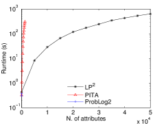
(a) Comparison.

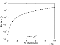
(b) LP² with up to $10^{5}$ attributes.

Figure 1: Runtime of LP², PITA and ProbLog2 on the workshops attributes problems. The Y-axis (runtime) is drawn in log scale. Note that, with the number of people fixed to 50, the problem is intractable by ProbLog2 which can manage at most two attributes.

Figure 2(a) shows the runtime of LP², PITA and ProbLog2 on the plates problem, while figure 2(b) shows that of LP² with up to $12\times 10^{4}$ $Y$ individuals. For this test we executed the query f and we fixed the number of different $X$ individuals to 5 and we increased the number of $Y$ individuals.

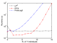
(a) Comparison.

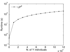
(b) LP² with up to $12\times 10^{4}$ Y individuals.

Figure 2: Performance on plates with an increasing number of $Y$ individuals. The Y-axis (runtime) is drawn in log scale.

Finally, we used the competing workshops problem for testing the scalability of LP². The trend was calculated performing the query series with 10 competing workshops and an increasing number $n$ of people problems. Figure 3 shows LP² computation time. The trend is almost linear in the number of people contained in the problem.

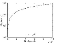
Figure 3: LP² runtime in the competing workshops problem. The Y-axis (runtime) is drawn in log scale.

As the results show, LP² can manage domains that are of several orders of magnitude larger than the ones managed by PITA and ProbLog2 in a shorter time.

6 Conclusions

We have shown that the Lifted Variable Elimination approach is very effective at resolving queries w.r.t. probabilistic logic programs containing large amount of facts. We have proved that with the introduction of the two new heterogeneous operators we can compute the probability of queries following the distribution semantics in a very efficient way. Experimental evidence shows that LP² can achieve several orders of magnitude improvements, both in runtime and in the number of facts that can be managed effectively. In the future, we plan to compare our approach with that of [Kisynski and Poole (2009b), Takikawa and D’Ambrosio (1999), Díez and Galán (2003)] for dealing with noisy or factors, and to compare with weighted first order model counting [Van den Broeck et al. (2014)].

Acknowledgments: VSC was partially financed by the North Portugal Regional Operational Programme (ON.2 – O Novo Norte), under the NSRF, through the ERDF and the Fundação para a Ciência e a Tecnologia within project ADE/PTDC/EIA-EIA/121686/2010. This work was supported by ”National Group of Computing Science (GNCS-INDAM)”.

Appendix A Problems code

In this section we present the Problog and PFL code of the testing problems.

A.1 Workshops Attributes

To all programs of this section we added 50 workshops and an increasing number of attributes.

Problog program

series:- person(P),attends(P),sa(P).

0.501::sa(P):-person(P).

attends(P):- person(P),attr(A),at(P,A).

0.3::at(P,A):-person(P),attr(A).

PFL program

het series1,ch1(P);[1.0, 0.0, 0.0, 1.0];[person(P)].

deputy series,series1;[].

bayes ch1(P),attends(P),sa(P);[1.0,1.0,1.0,0.0,
                               0.0,0.0,0.0,1.0];[person(P)].

bayes sa(P);[0.499,0.501];[person(P)].

het attends1(P),at(P,A);[1.0, 0.0, 0.0, 1.0];[person(P),attr(A)].

deputy attends(P),attends1(P);[person(P)].

bayes at(P,A);[0.7,0.3];[person(P),attr(A)].

A.2 Competing Workshops

For the competing workshops problem we report only the PFL version. For testing purpose we added to this code 10 workshops and an increasing number of people.

PFL program

bayes ch1(P),attends(P),sa(P);[1.0,1.0,1.0,0.0,
                               0.0,0.0,0.0,1.0];[person(P)].

het series1,ch1(P);[1.0, 0.0, 0.0, 1.0];[person(P)].

deputy series,series1;[].

bayes sa(P);[0.499,0.501];[person(P)].

het attends1(P),ch2(P,W);[1.0, 0.0, 0.0, 1.0];[person(P),workshop(W)].

deputy attends(P),attends1(P);[person(P)].

bayes ch2(P,W),hot(W),ah(P,W);[1.0,1.0,1.0,0.0,
                               0.0,0.0,0.0,1.0];[person(P),workshop(W)].

bayes ah(P,W);[0.2,0.8];[person(P),workshop(W)].

A.3 Plates

For tha plates problem we added 5 individuals for $X$ and an increasing number of individuals for $Y$.

Problog program

f:- e(Y).

e(Y) :- d(Y),n1(Y).
e(Y) :- y(Y),\+ d(Y),n2(Y).

d(Y):- c(X,Y).

c(X,Y):-b(X),n3(X,Y).
c(X,Y):- x(X),\+ b(X),n4(X,Y).

b(X):- a, n5(X).
b(X):- \+ a,n6(X).

a:- n7.

0.1::n1(Y) :-y(Y).
0.2::n2(Y) :-y(Y).
0.3::n3(X,Y) :- x(X),y(Y).
0.4::n4(X,Y) :- x(X),y(Y).
0.5::n5(X) :-x(X).
0.6::n6(X) :-x(X).
0.7::n7.

PFL program

het f1,e(Y);[1.0, 0.0, 0.0, 1.0];[y(Y)].

deputy f,f1;[].

bayes e1(Y),d(Y),n1(Y);[1.0, 1.0, 1.0, 0.0,
                        0.0, 0.0, 0.0, 1.0];[y(Y)].

bayes e2(Y),d(Y),n2(Y);[1.0, 0.0, 1.0, 1.0,
                        0.0, 1.0, 0.0, 0.0];[y(Y)].

bayes e(Y),e1(Y),e2(Y);[1.0, 0.0, 0.0, 0.0,
                        0.0, 1.0, 1.0, 1.0];[y(Y)].

het d1(Y),c(X,Y);[1.0, 0.0, 0.0, 1.0];[x(X),y(Y)].

deputy d(Y),d1(Y);[y(Y)].

bayes c1(X,Y),b(X),n3(X,Y);[1.0, 1.0, 1.0, 0.0,
                            0.0, 0.0, 0.0, 1.0];[x(X),y(Y)].

bayes c2(X,Y),b(X),n4(X,Y);[1.0, 0.0, 1.0, 1.0,
                            0.0, 1.0, 0.0, 0.0];[x(X),y(Y)].

bayes c(X,Y),c1(X,Y),c2(X,Y);[1.0, 0.0, 0.0, 0.0,
                              0.0, 1.0, 1.0, 1.0];[x(X),y(Y)].

bayes b1(X),a,n5(X);[1.0, 1.0, 1.0, 0.0,
                     0.0, 0.0, 0.0, 1.0];[x(X)].

bayes b2(X),a,n6(X);[1.0, 0.0, 1.0, 1.0,
                     0.0, 1.0, 0.0, 0.0];[x(X)].

bayes b(X),b1(X),b2(X);[1.0, 0.0, 0.0, 0.0,
                        0.0, 1.0, 1.0, 1.0];[x(X)].

bayes a,n7;[1.0, 0.0, 0.0, 1.0];[].

bayes n1(Y);[0.9, 0.1];[y(Y)].
bayes n2(Y);[0.8, 0.2];[y(Y)].
bayes n3(X,Y);[0.7, 0.3];[x(X),y(Y)].
bayes n4(X,Y);[0.6, 0.4];[x(X),y(Y)].
bayes n5(X);[0.5, 0.5];[x(X)].
bayes n6(X);[0.4, 0.6];[x(X)].
bayes n7;[0.3, 0.7];[].

Appendix B Definitions

Definition 1 (counting formula)

A counting formula is a syntactic construct of the form $\#_{X_{i}\in C}[F(\mathbf{X})]$, where $X_{i}\in\mathbf{X}$ is called the counted logvar.

A $grounded$ counting formula is a counting formula in which all arguments of the atom $F(\mathbf{X})$, except for the counted logvar, are constants. It defines a counting randvar (CRV) as follows.

Definition 2 (counting randvar)

A parametrized counting randvar (PCRV) is a pair ($\#_{X_{i}}[F(\mathbf{X})],C)$. For each instantiation of $\mathbf{X}\setminus X_{i}$, it creates a separate counting randvar (CRV). The value of this CRV is a histogram, and it depends deterministically on the values of $F(\mathbf{X})$. Given a valuation for $F(\mathbf{X})$, it counts how many different values of $X_{i}$ occur for each $r\in range(F)$. The result is a histogram of the form $\{(r_{1},n_{1}),\ldots,(r_{k},n_{k})\}$, with $r_{i}\in range(F)$ and $n_{i}$ the corresponding count.

Definition 3 (multiplicity)

The multiplicity of a histogram $h=\{(r1,n1),\ldots,(r_{k},n_{k})\}$ is a multinomial coefficient, defined as

$$\mbox{{\sc Mul}}(h)=\frac{n!}{\prod_{i=1}^{k}n_{i}!}.$$

As multiplicities should only be taken into account for (P)CRVs, never for regular PRVs, we define for each PRV $A$ and for each value $v\in range(A):\mbox{{\sc Mul}}(A,v)=1$ if $A$ is a regular PRV, and $\mbox{{\sc Mul}}(A,v)=\mbox{{\sc Mul}}(v)$ if $A$ is a PCRV. This Mul function is identical to [Milch et al. (2008)]’s num-assign.

Definition 4 (Count function)

Given a constraint $C_{\mathbf{X}}$, for any $\mathbf{Y}\subseteq\mathbf{X}$ and $\mathbf{Z}\subseteq\mathbf{X-Y}$, the function Count${}_{\mathbf{Y}|\mathbf{X}}:C_{\mathbf{X}}\rightarrow\mathbb{N}$ is defined as follows:

$$\mbox{{\sc{Count}}}_{\mathbf{Y}|\mathbf{Z}}(t)=|\pi_{\mathbf{Y}}(\sigma_{\mathbf{Z}=\pi_{\mathbf{Z}}(t)}(C_{\mathbf{X}}))|$$

That is, for any tuple t, this function tells us how many values for $\mathbf{Y}$ co-occur with t’s value for $\mathbf{Z}$ in the constraint. We define Count${}_{\mathbf{Y}|\mathbf{Z}}(t)=1$ when $\mathbf{Y}=\emptyset$.

Definition 5 (Count-normalized constraint)

For any constraint $C_{\mathbf{X}}$, $\mathbf{Y}\subseteq\mathbf{X}$ and $\mathbf{Z}\subseteq\mathbf{X-Y}$, $\mathbf{Y}$ is count-normalized w.r.t. $\mathbf{Z}$ in $C_{\mathbf{X}}$ if and only if

$$\exists n\in\mathbb{N}:\forall t\in C_{\mathbf{X}}:\mbox{{\sc{Count}}}_{\mathbf{Y}|\mathbf{Z}}(t)=n.$$

When such an $n$ exists, we call it the conditional count of $\mathbf{Y}$ given $\mathbf{Z}$ in $C_{\mathbf{X}}$, and denote it Count${}_{\mathbf{Y}|\mathbf{Z}}(C_{\mathbf{X}})$.

Definition 6 (substitution)

A substitution $\theta=\{X_{1}\rightarrow t_{1},\ldots,X_{n}\rightarrow t_{n}\}=\{\mathbf{X}\rightarrow\mathbf{t}\}$ maps each logvar $X_{i}$ to a term $t_{i}$, which can be a constant or a logvar. When all $t_{i}$ are constants, $\theta$ is called a grounding substitution, and when all are different logvars, a renaming substitution. Applying a substitution $\theta$ to an expression $\alpha$ means replacing each occurrence of $X_{i}$ in $\alpha$ with $t_{i}$; the result is denoted $\alpha\theta$.

Definition 7 (alignment)

An alignment $\theta$ between two parfactors $g=\phi(\mathcal{A})|C$ and $g^{\prime}=\phi^{\prime}(\mathcal{A}^{\prime})|C^{\prime}$ is a one-to-one substitution $\{\mathbf{X}\rightarrow\mathbf{X}^{\prime}\}$, with $\mathbf{X}\subseteq logvar(\mathcal{A})$ and $\mathbf{X^{\prime}}\subseteq logvar(\mathcal{A}^{\prime})$, such that $\rho(\pi_{\mathbf{X^{\prime}}}(C))=\pi_{\mathbf{X^{\prime}}}(C^{\prime})$ (with $\rho$ the attribute renaming operator).

An alignment tells the multiplication operator that two atoms in two different parfactors represent the same PRV, so it suffices to include it in the resulting parfactor only once.

Appendix C Correctness proof for heterogeneous multiplication

Theorem 1

Given a model $(\mathcal{F}_{1},\mathcal{F}_{2})$, two heterogeneous parfactors $g_{1},g_{2}\in\mathcal{F}_{2}$ and an alignment $\theta$ between $g_{1}$ and $g_{2}$, if the preconditions of the het-multiply operator are fulfilled then the postcondition

$$G\setminus\{g_{1},g_{2}\}\cup\{\textsc{het-multiply}(g_{1},g_{2},\theta)\}$$

holds.

Proof C.2.

Immediate from the definition of heterogeneous multiplication.

Theorem C.3.

Given a model $(\mathcal{F}_{1},\mathcal{F}_{2})$, a heterogeneous parfactor $g\in\mathcal{F}_{2}$ and an atom $A_{k+1}$ to be summed out, if the preconditions of the het-sum-out operator are fulfilled then the postcondition

$$\mathcal{P}_{G\setminus\{g\}\cup\{\textsc{het-sum-out}(g,(A_{1},\ldots,A_{k}),A_{k+1})\}}=\sum_{RV(A_{k+1})}\mathcal{P}_{\mathcal{G}}$$

holds.

Proof C.4.

We prove the formula giving $phi^{\prime}$ in Operator 2 by double induction over $r=\textsc{Count}_{\mathbf{X}^{excl}|\mathbf{X}^{com}}(C)$ and the number $n$ of values at $t$ in the tuple $(a^{\prime}_{1},\ldots,a^{\prime}_{k})$. For simplicity we assume that the variable to be summed out, $A_{k+1}$, is not a counting variable, but the same reasoning can be applied for a counting variable. For $n=0$, $r=1$

$$\phi^{\prime}(\textit{f},\ldots,\textit{f},\mathbf{b})=\phi(\textit{f},\ldots,\textit{f},\textit{f},\mathbf{b})+\phi(\textit{f},\ldots,\textit{f},t,\mathbf{b})$$

so the thesis is proved. For $n=0$, $r>1$, let us call $\phi^{\prime}_{r}(a^{\prime}_{1},\ldots,a^{\prime}_{k},\mathbf{b})$ the the value of $\phi^{\prime}$ for $r$. Let us assume that the formula holds for $r-1$. For $r>1$, there is an extra valuation $\mathbf{x}_{excl}$ for $\mathbf{X}_{excl}$ given $\mathbf{X}_{com}$ so there is an extra factor $g^{\prime\prime}(\mathbf{x}_{excl})$. Eliminating $A_{k+1}$ from $g^{\prime\prime}$ gives

$$\phi^{\prime}_{1}(\textit{f},\ldots,\textit{f},\mathbf{b})=\phi(\textit{f},\ldots,\textit{f},\textit{f},\mathbf{b})+\phi(\textit{f},\ldots,\textit{f},\textit{t},\mathbf{b})$$

This must be multiplied by $\phi^{\prime}_{r-1}$ with heterogeneous multiplication as $A_{1},\ldots,A_{k}$ are shared obtaining

$$\phi^{\prime}_{r}(\textit{f},\ldots,\textit{f},\mathbf{b})=\sum_{\hat{a}_{1}\vee\check{a}_{1}=\textit{f}}\ldots\sum_{\hat{a}_{k}\vee\check{a}_{k}=\textit{f}}\phi^{\prime}_{r-1}(\hat{a}_{1},\ldots,\hat{a}_{k},\mathbf{b})\times\phi^{\prime}_{1}(\check{a}_{1},\ldots,\check{a}_{k},\textit{f},\mathbf{b})=$$

$$=\phi^{\prime}_{r-1}(\textit{f},\ldots,\textit{f},\mathbf{b})\times\phi^{\prime}_{1}(\check{a}_{1},\ldots,\check{a}_{k},\textit{f},\mathbf{b})=$$

$$=(\phi(\textit{f},\ldots,\textit{f},\textit{f},\mathbf{b})+\phi(\textit{f},\ldots,\textit{f},\textit{t},\mathbf{b}))^{r-1}\times(\phi(\textit{f},\ldots,\textit{f},\textit{f},\mathbf{b})+\phi(\textit{f},\ldots,\textit{f},\textit{t},\mathbf{b}))=$$

$$=(\phi(\textit{f},\ldots,\textit{f},\textit{f},\mathbf{b})+\phi(\textit{f},\ldots,\textit{f},\textit{t},\mathbf{b}))^{r}$$

so the thesis is proved.

For $n>0$ of values at $t$ in the tuple $\mathbf{a}^{\prime}=(a^{\prime}_{1},\ldots,a^{\prime}_{k})$, we assume that the formula holds for $(n-1,r)$ and $(n,r-1)$. For the defintiion of heterogeneous multiplication

$$\phi^{\prime}_{r}(a^{\prime}_{1},\ldots,a^{\prime}_{k},\mathbf{b}) = \sum_{\hat{a}_{1}\vee\check{a}_{1}=a^{\prime}_{1}}\ldots\sum_{\hat{a}_{k}\vee\check{a}_{k}=a^{\prime}_{k}}\phi^{\prime}_{r-1}(\hat{a}_{1},\ldots,\hat{a}_{k},\mathbf{b})\phi^{\prime}_{1}(\check{a}_{1},\ldots,\check{a}_{k},\mathbf{b})$$

By adding and removing

$\sum_{\mathbf{a}<\mathbf{a}^{\prime}}\sum_{\hat{a}_{1}\vee\check{a}_{1}=a_{1}}\ldots\sum_{\hat{a}_{k}\vee\check{a}_{k}=a_{k}}\phi^{\prime}_{r-1}(\hat{a}_{1},\ldots,\hat{a}_{k},\mathbf{b})\phi^{\prime}_{1}(\check{a}_{1},\ldots,\check{a}_{k},\mathbf{b})$

we get

$\phi^{\prime}_{r}(a^{\prime}_{1},\ldots,a^{\prime}_{k},\mathbf{b})=$

$$= \sum_{\hat{a}_{1}\vee\check{a}_{1}=a^{\prime}_{1}}\ldots\sum_{\hat{a}_{k}\vee\check{a}_{k}=a^{\prime}_{k}}\phi^{\prime}_{r-1}(\hat{a}_{1},\ldots,\hat{a}_{k},\mathbf{b})\phi^{\prime}_{1}(\check{a}_{1},\ldots,\check{a}_{k},\mathbf{b})+$$

$$+\sum_{\mathbf{a}<\mathbf{a}^{\prime}}\sum_{\hat{a}_{1}\vee\check{a}_{1}=a_{1}}\ldots\sum_{\hat{a}_{k}\vee\check{a}_{k}=a_{k}}\phi^{\prime}_{r-1}(\hat{a}_{1},\ldots,\hat{a}_{k},\mathbf{b})\phi^{\prime}_{1}(\check{a}_{1},\ldots,\check{a}_{k},\mathbf{b})-$$

$$-\sum_{\mathbf{a}<\mathbf{a}^{\prime}}\sum_{\hat{a}_{1}\vee\check{a}_{1}=a_{1}}\ldots\sum_{\hat{a}_{k}\vee\check{a}_{k}=a_{k}}\phi^{\prime}_{r-1}(\hat{a}_{1},\ldots,\hat{a}_{k},\mathbf{b})\phi^{\prime}_{1}(\check{a}_{1},\ldots,\check{a}_{k},\mathbf{b})=$$

$$= \sum_{\hat{a}_{1}\leq a^{\prime}_{1}}\sum_{\check{a}_{1}\leq a^{\prime}_{1}}\ldots\sum_{\hat{a}_{k}\leq a^{\prime}_{k}}\sum_{\check{a}_{k}\leq a^{\prime}_{k}}\phi^{\prime}_{r-1}(\hat{a}_{1},\ldots,\hat{a}_{k},\mathbf{b})\phi^{\prime}_{1}(\check{a}_{1},\ldots,\check{a}_{k},\mathbf{b})-$$

$$-\sum_{\mathbf{a}<\mathbf{a}^{\prime}}\sum_{\hat{a}_{1}\vee\check{a}_{1}=a_{1}}\ldots\sum_{\hat{a}_{k}\vee\check{a}_{k}=a_{k}}\phi^{\prime}_{r-1}(\hat{a}_{1},\ldots,\hat{a}_{k},\mathbf{b})\phi^{\prime}_{1}(\check{a}_{1},\ldots,\check{a}_{k},\mathbf{b})=$$

For the definition of heterogeneous multiplication we obtain $\phi^{\prime}_{r}(a^{\prime}_{1},\ldots,a^{\prime}_{k},\mathbf{b})=$

$$= \left(\sum_{\hat{\mathbf{a}}\leq\mathbf{a}^{\prime}}\phi^{\prime}_{r-1}(\hat{a}_{1},\ldots,\hat{a}_{k},\mathbf{b})\right)\times\left(\sum_{\check{\mathbf{a}}\leq\mathbf{a}^{\prime}}\phi^{\prime}_{1}(\check{a}_{1},\ldots,\check{a}_{k},\mathbf{b})\right)-\sum_{\mathbf{a}<\mathbf{a}^{\prime}}\phi^{\prime}_{r}(a_{1},\ldots,a_{k},\mathbf{b})$$

By applying the inductive hypothesis for $r-1$ we get $\phi^{\prime}_{r}(a^{\prime}_{1},\ldots,a^{\prime}_{k},\mathbf{b})=$

$$= \left(\sum_{\hat{\mathbf{a}}\leq\mathbf{a}^{\prime}}\left(\sum_{\mathbf{a}\leq\hat{\mathbf{a}}}\phi(a_{1},\ldots,a_{k},\textit{f},\mathbf{b})+\phi(a_{1},\ldots,a_{k},\textit{t},\mathbf{b})\right)^{r-1}-\sum_{\mathbf{a}<\hat{\mathbf{a}}}\phi^{\prime}_{r-1}(a_{1},\ldots,a_{k},\mathbf{b})\right)\times$$

$$\times\left(\sum_{\check{\mathbf{a}}\leq\mathbf{a}^{\prime}}\phi^{\prime}_{1}(\check{a}_{1},\ldots,\check{a}_{k},\mathbf{b})\right)-\sum_{\mathbf{a}<\mathbf{a}^{\prime}}\phi^{\prime}_{r}(a_{1},\ldots,a_{k},\mathbf{b})=$$

$$= \left(\sum_{\hat{\mathbf{a}}\leq\mathbf{a}^{\prime}}\left(\sum_{\mathbf{a}\leq\hat{\mathbf{a}}}\phi(a_{1},\ldots,a_{k},\textit{f},\mathbf{b})+\phi(a_{1},\ldots,a_{k},\textit{t},\mathbf{b})\right)^{r-1}\right)\times\left(\sum_{\check{\mathbf{a}}\leq\mathbf{a}^{\prime}}\phi^{\prime}_{1}(\check{a}_{1},\ldots,\check{a}_{k},\mathbf{b})\right)-$$

$$-\left(\sum_{\hat{\mathbf{a}}\leq\mathbf{a}^{\prime}}\sum_{\mathbf{a}<\hat{\mathbf{a}}}\phi^{\prime}_{r-1}(a_{1},\ldots,a_{k},\mathbf{b})\right)\times\left(\sum_{\check{\mathbf{a}}\leq\mathbf{a}^{\prime}}\phi^{\prime}_{1}(\check{a}_{1},\ldots,\check{a}_{k},\mathbf{b})\right)$$

$$-\sum_{\mathbf{a}<\mathbf{a}^{\prime}}\phi^{\prime}_{r}(a_{1},\ldots,a_{k},\mathbf{b})=$$

$$= \left(\sum_{\mathbf{a}\leq\mathbf{a}^{\prime}}\phi(a_{1},\ldots,a_{k},\textit{f},\mathbf{b})+\phi(a_{1},\ldots,a_{k},\textit{t},\mathbf{b})\right)^{r-1}\times\left(\sum_{\mathbf{a}\leq\mathbf{a}^{\prime}}\phi^{\prime}_{1}(\check{a}_{1},\ldots,\check{a}_{k},\mathbf{b})\right)+$$

$$+\left(\sum_{\hat{\mathbf{a}}<\mathbf{a}^{\prime}}\left(\sum_{\mathbf{a}\leq\hat{\mathbf{a}}}\phi(a_{1},\ldots,a_{k},\textit{f},\mathbf{b})+\phi(a_{1},\ldots,a_{k},\textit{t},\mathbf{b})\right)^{r-1}\right)\times\left(\sum_{\check{\mathbf{a}}\leq\mathbf{a}^{\prime}}\phi^{\prime}_{1}(\check{a}_{1},\ldots,\check{a}_{k},\mathbf{b})\right)-$$

$$-\left(\sum_{\hat{\mathbf{a}}\leq\mathbf{a}^{\prime}}\sum_{\mathbf{a}<\hat{\mathbf{a}}}\phi^{\prime}_{r-1}(a_{1},\ldots,a_{k},\mathbf{b})\right)\times\left(\sum_{\check{\mathbf{a}}\leq\mathbf{a}^{\prime}}\phi^{\prime}_{1}(\check{a}_{1},\ldots,\check{a}_{k},\mathbf{b})\right)-$$

$$-\sum_{\mathbf{a}<\mathbf{a}^{\prime}}\phi^{\prime}_{r}(a_{1},\ldots,a_{k},\mathbf{b})=$$

By applying the formula for $r=1$
$\phi^{\prime}_{r}(a^{\prime}_{1},\ldots,a^{\prime}_{k},\mathbf{b})=$

$$= \left(\sum_{\mathbf{a}\leq\mathbf{a}^{\prime}}\phi(a_{1},\ldots,a_{k},\textit{f},\mathbf{b})+\phi(a_{1},\ldots,a_{k},\textit{t},\mathbf{b})\right)^{r-1}\times\left(\sum_{\mathbf{a}\leq\mathbf{a}^{\prime}}\phi(a_{1},\ldots,a_{k},\textit{f},\mathbf{b})+\phi(a_{1},\ldots,a_{k},\textit{t},\mathbf{b})\right)+$$

$$+\left(\sum_{\hat{\mathbf{a}}<\mathbf{a}^{\prime}}\left(\sum_{\mathbf{a}\leq\hat{\mathbf{a}}}\phi(a_{1},\ldots,a_{k},\textit{f},\mathbf{b})+\phi(a_{1},\ldots,a_{k},\textit{t},\mathbf{b})\right)^{r-1}\right)\times\left(\sum_{\check{\mathbf{a}}\leq\mathbf{a}^{\prime}}\phi^{\prime}_{1}(\check{a}_{1},\ldots,\check{a}_{k},\mathbf{b})\right)-$$

$$-\left(\sum_{\hat{\mathbf{a}}<\mathbf{a}^{\prime}}\sum_{\mathbf{a}<\hat{\mathbf{a}}}\phi^{\prime}_{r-1}(a_{1},\ldots,a_{k},\mathbf{b})\right)\times\left(\sum_{\check{\mathbf{a}}\leq\mathbf{a}^{\prime}}\phi^{\prime}_{1}(\check{a}_{1},\ldots,\check{a}_{k},\mathbf{b})\right)-$$

$$-\sum_{\mathbf{a}<\mathbf{a}^{\prime}}\phi^{\prime}_{r}(a_{1},\ldots,a_{k},\mathbf{b})=$$

$$= \left(\sum_{\mathbf{a}\leq\mathbf{a}^{\prime}}\phi(a_{1},\ldots,a_{k},\textit{f},\mathbf{b})+\phi(a_{1},\ldots,a_{k},\textit{t},\mathbf{b})\right)^{r}-\sum_{\mathbf{a}<\mathbf{a}^{\prime}}\phi^{\prime}_{r}(a_{1},\ldots,a_{k},\mathbf{b})+$$

$$+\left(\sum_{\hat{\mathbf{a}}<\mathbf{a}^{\prime}}\left(\sum_{\mathbf{a}\leq\hat{\mathbf{a}}}\phi(a_{1},\ldots,a_{k},\textit{f},\mathbf{b})+\phi(a_{1},\ldots,a_{k},\textit{t},\mathbf{b})\right)^{r-1}\right)\times\left(\sum_{\check{\mathbf{a}}\leq\mathbf{a}^{\prime}}\phi^{\prime}_{1}(\check{a}_{1},\ldots,\check{a}_{k},\mathbf{b})\right)-$$

$$-\left(\sum_{\hat{\mathbf{a}}<\mathbf{a}^{\prime}}\sum_{\mathbf{a}<\hat{\mathbf{a}}}\phi^{\prime}_{r-1}(a_{1},\ldots,a_{k},\mathbf{b})\right)\times\left(\sum_{\check{\mathbf{a}}\leq\mathbf{a}^{\prime}}\phi^{\prime}_{1}(\check{a}_{1},\ldots,\check{a}_{k},\mathbf{b})\right)$$

By collecting the factor $\sum_{\check{\mathbf{a}}\leq\mathbf{a}^{\prime}}\phi^{\prime}_{1}(\check{a}_{1},\ldots,\check{a}_{k},\mathbf{b})$ $\phi^{\prime}_{r}(a^{\prime}_{1},\ldots,a^{\prime}_{k},\mathbf{b})=$

$$= \left(\sum_{\mathbf{a}\leq\mathbf{a}^{\prime}}\phi(a_{1},\ldots,a_{k},\textit{f},\mathbf{b})+\phi(a_{1},\ldots,a_{k},\textit{t},\mathbf{b})\right)^{r}-\sum_{\mathbf{a}<\mathbf{a}^{\prime}}\phi^{\prime}_{r}(a_{1},\ldots,a_{k},\mathbf{b})+$$

$$+\left(\sum_{\hat{\mathbf{a}}<\mathbf{a}^{\prime}}\left(\sum_{\mathbf{a}\leq\hat{\mathbf{a}}}\phi(a_{1},\ldots,a_{k},\textit{f},\mathbf{b})+\phi(a_{1},\ldots,a_{k},\textit{t},\mathbf{b})\right)^{r-1}-\sum_{\hat{\mathbf{a}}<\mathbf{a}^{\prime}}\sum_{\mathbf{a}\leq\hat{\mathbf{a}}}\phi^{\prime}_{r-1}(a_{1},\ldots,a_{k},\mathbf{b})\right)\times$$

$$\times\left(\sum_{\check{\mathbf{a}}\leq\mathbf{a}^{\prime}}\phi^{\prime}_{1}(\check{a}_{1},\ldots,\check{a}_{k},\mathbf{b})\right)=$$

$$= \left(\sum_{\mathbf{a}\leq\mathbf{a}^{\prime}}\phi(a_{1},\ldots,a_{k},\textit{f},\mathbf{b})+\phi(a_{1},\ldots,a_{k},\textit{t},\mathbf{b})\right)^{r}-\sum_{\mathbf{a}<\mathbf{a}^{\prime}}\phi^{\prime}_{r}(a_{1},\ldots,a_{k},\mathbf{b})+$$

$$+\left(\sum_{\hat{\mathbf{a}}<\mathbf{a}^{\prime}}\left(\sum_{\mathbf{a}\leq\hat{\mathbf{a}}}\phi(a_{1},\ldots,a_{k},\textit{f},\mathbf{b})+\phi(a_{1},\ldots,a_{k},\textit{t},\mathbf{b})\right)^{r-1}-\sum_{\hat{\mathbf{a}}<\mathbf{a}^{\prime}}\sum_{\mathbf{a}<\hat{\mathbf{a}}}\phi^{\prime}_{r-1}(a_{1},\ldots,a_{k},\mathbf{b})-\right.$$

$$\left.-\sum_{\mathbf{a}<\mathbf{a}^{\prime}}\phi^{\prime}_{r-1}(a_{1},\ldots,a_{k},\mathbf{b})\right)\times(\sum_{\mathbf{a}\leq\mathbf{a}^{\prime}}\phi^{\prime}_{1}(a_{1},\ldots,a_{k},\mathbf{b}))=$$

$$= \left(\sum_{\mathbf{a}\leq\mathbf{a}^{\prime}}\phi(a_{1},\ldots,a_{k},\textit{f},\mathbf{b})+\phi(a_{1},\ldots,a_{k},\textit{t},\mathbf{b})\right)^{r}-\sum_{\mathbf{a}<\mathbf{a}^{\prime}}\phi^{\prime}_{r}(a_{1},\ldots,a_{k},\mathbf{b})+$$

$$+\left(\sum_{\mathbf{a}<\mathbf{a}^{\prime}}\phi^{\prime}_{r-1}(a_{1},\ldots,a_{k},\mathbf{b})-\sum_{\mathbf{a}<\mathbf{a}^{\prime}}\phi^{\prime}_{r-1}(a_{1},\ldots,a_{k},\mathbf{b})\right)\times\sum_{\mathbf{a}\leq\mathbf{a}^{\prime}}\phi^{\prime}_{1}(a_{1},\ldots,a_{k},\mathbf{b})=$$

$$= \left(\sum_{\mathbf{a}\leq\mathbf{a}^{\prime}}\phi(a_{1},\ldots,a_{k},\textit{f},\mathbf{b})+\phi(a_{1},\ldots,a_{k},\textit{t},\mathbf{b})\right)^{r}-\sum_{\mathbf{a}<\mathbf{a}^{\prime}}\phi^{\prime}_{r}(a_{1},\ldots,a_{k},\mathbf{b})$$

References

• De Raedt et al. (2008) De Raedt, L., Frasconi, P., Kersting, K., and Muggleton, S., Eds. 2008. Probabilistic Inductive Logic Programming - Theory and Applications. LNCS, vol. 4911. Springer.
• De Raedt et al. (2007) De Raedt, L., Kimmig, A., and Toivonen, H. 2007. ProbLog: A Probabilistic Prolog and its application in link discovery. In 20th International Joint Conference on Artificial Intelligence (IJCAI-2007). AAAI Press, 2462–2467.
• de Salvo Braz et al. (2005) de Salvo Braz, R., Amir, E., and Roth, D. 2005. Lifted first-order probabilistic inference. In 19th International Joint Conference on Artificial Intelligence, L. P. Kaelbling and A. Saffiotti, Eds. Professional Book Center, 1319–1325.
• Díez and Galán (2003) Díez, F. J. and Galán, S. F. 2003. Efficient computation for the noisy max. International Journal of Intelligent Systems, 165–177.
• Fierens et al. (2014) Fierens, D., Van den Broeck, G., Renkens, J., Shterionov, D., Gutmann, B., Thon, I., Janssens, G., and De Raedt, L. 2014. Inference and learning in probabilistic logic programs using weighted boolean formulas. Theory and Practice of Logic Programming FirstView Articles.
• Getoor and Taskar (2007) Getoor, L. and Taskar, B., Eds. 2007. Introduction to Statistical Relational Learning. MIT Press.
• Gomes and Costa (2012) Gomes, T. and Costa, V. S. 2012. Evaluating inference algorithms for the prolog factor language. In 22nd International Conference on Inductive Logic Programming, F. Riguzzi and F. Zelezný, Eds. LNCS, vol. 7842. Springer, 74–85.
• Kisynski and Poole (2009a) Kisynski, J. and Poole, D. 2009a. Constraint processing in lifted probabilistic inference. In 25th Conference on Uncertainty in Artificial Intelligence, J. Bilmes and A. Y. Ng, Eds. AUAI Press, 293–302.
• Kisynski and Poole (2009b) Kisynski, J. and Poole, D. 2009b. Lifted aggregation in directed first-order probabilistic models. In 24th International Joint Conference on Artificial Intelligence, C. Boutilier, Ed. 1922–1929.
• Meert et al. (2008) Meert, W., Struyf, J., and Blockeel, H. 2008. Learning ground CP-Logic theories by leveraging Bayesian network learning techniques. Fundamenta Informaticae 89, 131–160.
• Milch et al. (2008) Milch, B., Zettlemoyer, L. S., Kersting, K., Haimes, M., and Kaelbling, L. P. 2008. Lifted probabilistic inference with counting formulas. In 23rd AAAI Conference on Artificial Intelligence, D. Fox and C. P. Gomes, Eds. AAAI Press, 1062–1068.
• Poole (1993) Poole, D. 1993. Probabilistic horn abduction and Bayesian networks. Artificial Intelligence 64, 1, 81–129.
• Poole (1997) Poole, D. 1997. The Independent Choice Logic for modelling multiple agents under uncertainty. Artificial Intelligence 94, 7–56.
• Poole (2003) Poole, D. 2003. First-order probabilistic inference. In 18th International Joint Conference on Artificial Intelligence, G. Gottlob and T. Walsh, Eds. Morgan Kaufmann Publishers Inc., 985–991.
• Poole (2008) Poole, D. 2008. The independent choice logic and beyond. In Probabilistic Inductive Logic Programming, L. De Raedt, P. Frasconi, K. Kersting, and S. Muggleton, Eds. LNCS, vol. 4911. Springer, 222–243.
• Riguzzi and Swift (2011) Riguzzi, F. and Swift, T. 2011. The PITA system: Tabling and answer subsumption for reasoning under uncertainty. Theory and Practice of Logic Programming, International Conference on Logic Programming (ICLP) Special Issue 11, 433–449.
• Sato (1995) Sato, T. 1995. A statistical learning method for logic programs with distribution semantics. In 12th International Conference on Logic Programming, L. Sterling, Ed. MIT Press, 715–729.
• Taghipour et al. (2013) Taghipour, N., Fierens, D., Davis, J., and Blockeel, H. 2013. Lifted variable elimination: Decoupling the operators from the constraint language. Journal of Artificial Intelligence Research 47, 393–439.
• Takikawa and D’Ambrosio (1999) Takikawa, M. and D’Ambrosio, B. 1999. Multiplicative factorization of noisy-max. In 15th Conference on Uncertainty in Artificial Intelligence. 622–630.
• Van den Broeck et al. (2014) Van den Broeck, G., Meert, W., and Darwiche, A. 2014. Skolemization for weighted first-order model counting. ArXiv e-prints 1312.5378v2. To appear in the 14th International Conference on Principles of Knowledge Representation and Reasoning.
• Van den Broeck et al. (2011) Van den Broeck, G., Taghipour, N., Meert, W., Davis, J., and Raedt, L. D. 2011. Lifted probabilistic inference by first-order knowledge compilation. In 21st International Joint Conference on Artificial Intelligence, T. Walsh, Ed. IJCAI/AAAI, 2178–2185.
• Vennekens et al. (2004) Vennekens, J., Verbaeten, S., and Bruynooghe, M. 2004. Logic Programs With Annotated Disjunctions. In 20th International Conference on Logic Programming, B. Demoen and V. Lifschitz, Eds. Springer, LNCS 3131, 195–209.
• Zhang and Poole (1996) Zhang, N. L. and Poole, D. L. 1996. Exploiting causal independence in bayesian network inference. Journal of Artificial Intelligence Research 5, 301–328.