Efficient Implementations of the Generalized Lasso Dual Path Algorithm

Abstract

We consider efficient implementations of the generalized lasso dual path algorithm of Tibshirani & Taylor (2011). We first describe a generic approach that covers any penalty matrix $D$ and any (full column rank) matrix $X$ of predictor variables. We then describe fast implementations for the special cases of trend filtering problems, fused lasso problems, and sparse fused lasso problems, both with $X=I$ and a general matrix $X$. These specialized implementations offer a considerable improvement over the generic implementation, both in terms of numerical stability and efficiency of the solution path computation. These algorithms are all available for use in the genlasso R package, which can be found in the CRAN repository.

Keywords: generalized lasso, trend filtering, fused lasso, path algorithm, QR decomposition, Laplacian linear systems

1 Introduction

In this article, we study computation in the generalized lasso problem (Tibshirani & Taylor, 2011)

$$\hat{\beta}=\mathop{\mathrm{arg\,min}}_{\beta\in\mathbb{R}^{p}}\,\frac{1}{2}\|y-X\beta\|_{2}^{2}+\lambda\|D\beta\|_{1},$$ (1)

where $y\in\mathbb{R}^{n}$ is an outcome vector, $X\in\mathbb{R}^{n\times p}$ is a predictor matrix, $D\in\mathbb{R}^{m\times p}$ is a penalty matrix, and $\lambda\geq 0$ is a regularization parameter. The term “generalized” refers to the fact that problem (1) reduces to the standard lasso problem (Tibshirani, 1996; Chen et al., 1998) when $D=I$, but yields different problems with different choices of the penalty matrix $D$. We will assume that $X$ has full column rank (i.e., $\mathrm{rank}(X)=p$), so as to ensure a unique solution in (1) for all values of $\lambda$.

Our main contribution is to derive efficient implementations of the generalized lasso dual path algorithm of Tibshirani & Taylor (2011). This algorithm computes the solution $\hat{\beta}(\lambda)$ in (1) over the full range of regularization parameter values $\lambda\in[0,\infty)$. We present an efficient implementation for a general penalty matrix $D$, as well as specialized, extra-efficient implementations for two special classes of generalized lasso problems: fused lasso and trend filtering problems. The algorithms that we describe in this work are all implemented in the genlasso R package, freely available on the CRAN repository (R Development Core Team, 2008).

We note that the fused lasso and trend filtering problems are known, well-established problems (early references for fused lasso are Land & Friedman (1996), Tibshirani et al. (2005), and early works on trend filtering are Steidl et al. (2006), Kim et al. (2009)). These problems are not original to the generalized lasso framework, but the latter framework simply provides a useful, unifying perspective from which we can study them. We give a brief overview here; see the aforementioned references for more discussion, or Section 2 of Tibshirani & Taylor (2011), and also Section 6 of this paper, for examples and figures.

In the first problem class, the fused lasso setting, we think of the components of $\beta\in\mathbb{R}^{p}$ as corresponding to the nodes of a given undirected graph $G$, with edge set $E\subseteq\{1,\ldots p\}^{2}$. If $E$ has $m$ edges, enumerated $e_{1},\ldots e_{m}$, then the fused lasso penalty matrix $D$ is $m\times p$, with one row for each edge in $E$. In particular, if $e_{\ell}=(i,j)$, then the $\ell$th row of $D$ is

$$D_{\ell}=(0,\ldots\underset{\begin{subarray}{c}\;\;\uparrow\\ \;\;i\end{subarray}}{-1},\ldots\underset{\begin{subarray}{c}\uparrow\\ j\end{subarray}}{1},\ldots 0)\in\mathbb{R}^{p},$$

i.e., $D_{\ell}$ contains all zeros except for a $-1$ and $1$ in the $i$th and $j$th components (equivalent to this would be a $1$ and $-1$ in the $i$th and $j$th components). The fused lasso penalty term is hence

$$\|D\beta\|_{1}=\sum_{e_{\ell}=(i,j)\in E}|\beta_{i}-\beta_{j}|.$$

The effect of this penalty in (1) is that many of the terms $|\hat{\beta}_{i}-\hat{\beta}_{j}|$ will be zero at the solution $\hat{\beta}$; in other words, the solution exhibits a piecewise constant structure over connected subgraphs of $G$. To relate the fused lasso penalty matrix to concepts from graph theory, note that $D$ as described above is the oriented incidence matrix of the undirected graph $G$. This means that $L=D^{T}D$ is the Laplacian matrix of $G$—a realization that will be useful for our work in Section 4.

An important special case to mention is the 1-dimensional fused lasso, in which the components of $\beta$ correspond to successive positions on a 1-dimensional grid, so $G$ is the chain graph (with edges $(i,i+1)$, $i=1,\ldots p-1$), and the penalty matrix is

$$D=\left[\begin{array}[]{rrrrrr}-1&1&0&\ldots&0&0\\ 0&-1&1&\ldots&0&0\\ \vdots&&&&&\\ 0&0&0&\ldots&-1&1\end{array}\right].$$ (2)

The solution $\hat{\beta}$ is therefore piecewise constant across the underlying positions. (A clarifying note: the original work of Land & Friedman (1996), Tibshirani et al. (2005) considered only this 1-dimensional setup, and the generalization to a graph setting came in later works. Also, Tibshirani et al. (2005) defined the fused lasso criterion with an additional $\ell_{1}$ penalty on coefficients $\beta$ themselves; we now refer to this as the sparse fused lasso problem. It is not fundamentally different from the version we consider here, with pure fusion, and can be handled by the described path algorithm; see Section 4.3.)

The second problem class, trend filtering, also starts with the assumption that the components of $\beta$ correspond to positions on an underlying 1d grid, like the 1d fused lasso; but trend filtering more generally produces a solution $\hat{\beta}$ that bears the structure of a piecewise $k$th degree polynomial function over the underlying positions, where $k\geq 0$ is a given integer. To accomplish this, the trend filtering penalty matrix is taken to be $D=D^{(k+1)}$, the $(p-k-1)\times p$ discrete difference operator of order $k+1$. These discrete derivative operators can be defined recursively, by letting $D^{(1)}$ be the $(p-1)\times p$ first difference matrix in (2), and

$$D^{(k+1)}=D^{(1)}D^{(k)}\;\;\;\text{for}\;\,k=1,2,3,\ldots.$$

(In the above, $D^{(1)}$ is the $(p-k-1)\times(p-k)$ version of the first difference matrix.) Note that the 1d fused lasso is exactly a special case of trend filtering with $k=0$. For a general order $k\geq 0$, the matrix $D^{(k+1)}$ is banded with bandwidth $k+2$, and a straightforward calculation shows that the penalty term in (1) can be written explicitly as

$$\|D^{(k+1)}\beta\|_{1}=\sum_{i=1}^{p-k-1}\left|\sum_{j=i}^{i+k+1}(-1)^{j-i}{k+1\choose j-i}\beta_{j}\right|.$$

We refer the reader to Tibshirani (2014) for a study of trend filtering as a signal estimation method (i.e., for $X=I$), where it is shown to have desirable statistical properties in a nonparametric regression context.

In what follows, we describe the dual path algorithm of Tibshirani & Taylor (2011), and then begin discussing strategies for its implementation. First, though, we briefly review other computational approaches for the generalized lasso problem (1).

1.1 Related work

There are many algorithms, aside from the dual path algorithm central to this paper, for solving the convex problem (1) and its various special cases. It will be helpful to distinguish between algorithms that solve (1) at fixed values of the tuning parameter $\lambda$, and algorithms that sweep out the entire path of solutions as a continuous function of $\lambda$.

In the former case, when the solution is desired a fixed value of $\lambda$, a number of more or less standard convex optimization techniques can be applied. For arbitrary matrices $X,D$, problem (1) can be recast as a quadratic program, so that, e.g., we may use the standard interior point methods common to quadratic and conic programming problems. We can also use the alternating direction method of multipliers (ADMM) for general $X,D$. For certain instantiations of $X,D$, there are faster, more specialized techniques. For example, when $X=I$ and $D$ is the 1d fused lasso matrix, problem (1) can be solved in linear time via a taut string method (Davies & Kovac, 2001), or dynamic programming (Johnson, 2013). When $X=I$ and $D$ is the fused lasso matrix over a graph, a clever parametric max flow approach (Chambolle & Darbon, 2009) applies. When $X=I$ and $D$ is the trend filtering matrix, highly efficient and specialized interior point methods (Kim et al., 2009) or ADMM algorithms (Ramdas & Tibshirani, 2014) are available. Finally, when $X$ is an arbitrary matrix and $D$ falls into any one of the above categories, one can implement a proximal gradient algorithm, with each proximal evaluation utilizing one of the specialized techniques just described.

In terms of path algorithms, the literature is more sparse. For the lasso problem, the well-known least angle regression algorithm of Efron et al. (2004) computes the full solution path (see also Osborne et al. (2000a, b)). For fused lasso problems, Hoefling (2010) describes a path algorithm based on max flow subroutines, which efficiently tracks the path in the direction opposite to the one we consider (i.e., starts with $\lambda=0$ and ends at $\lambda=\infty$). For the generalized lasso problem, Zhou & Lange (2013) propose a path algorithm from the primal perspective; however, their work assumes $D$ to have full row rank, which does not hold in many cases of interest (such as the fused lasso over a graph with more edges than nodes). The dual path algorithm of Tibshirani & Taylor (2011) has the advantage that it operates in a single, unified framework that allows $D$ to be completely general, but is also flexible enough to permit efficient specialized versions when $D$ takes specific forms. Given the magnitude of related work, we do not give detailed comparisons to alternative methods, but instead focus on fast, stable implementations of the generalized lasso dual path algorithm.

1.2 The dual path algorithm

We recall the details of the dual path algorithm for the generalized lasso problem. We do not place any assumptions on $D\in\mathbb{R}^{m\times n}$, but we do assume that $X$ has full column rank, which implies a unique solution in (1) for all $\lambda$. As its name suggests, the dual path algorithm actually computes a solution path of the equivalent dual problem of (1), instead of solving (1) directly.

1.2.1 The signal approximator case, $X=I$

It helps to first consider the “signal approximator” case, $X=I$. In this case, for any fixed value of $\lambda$, the dual of problem (1) is:

$$\hat{u}\in\mathop{\mathrm{arg\,min}}_{u\in\mathbb{R}^{m}}\,\frac{1}{2}\|y-D^{T}u\|_{2}^{2}\;\;\mathop{\mathrm{subject\,\,to}}\;\,\|u\|_{\infty}\leq\lambda,$$ (3)

and the primal and dual solutions, $\hat{\beta}$ and $\hat{u}$, are related by:

$$\hat{\beta}=y-D^{T}\hat{u}.$$ (4)

We note that, though the primal solution is unique, the dual solution need not be unique (this is reflected by the element notation in (3)).

The path algorithm proposed Tibshirani & Taylor (2011) computes a solution path $\hat{u}(\lambda)$ of the dual problem, beginning at $\lambda=\infty$ and progressing down to $\lambda=0$; this gives the primal solution path $\hat{\beta}(\lambda)$ using the transformation in (4). At a high level, the algorithm keeps track of the coordinates of the computed dual solution $\hat{u}(\lambda)$ that are equal to $\pm\lambda$, i.e., that lie on the boundary of the constraint region $[-\lambda,\lambda]^{m}$, and it determines critical values of the regularization parameter, $\lambda_{1}\geq\lambda_{2}\geq\ldots$, at which coordinates of this solution hit or leave the boundary. We outline the algorithm below; in terms of notation, we write $D_{S}$ to extract the rows of $D$ in $S\subseteq\{1,\ldots m\}$, and we use $D_{-S}$ as shorthand for $D_{\{1,\ldots m\}\setminus S}$.

Algorithm 1 (Dual path algorithm for the generalized lasso, $X=I$).

Given $y\in\mathbb{R}^{n}$ and $D\in\mathbb{R}^{m\times n}$.

1. Compute $\hat{u}$, the minimum $\ell_{2}$ norm solution of

   $$\min_{u\in\mathbb{R}^{m}}\,\|y-D^{T}u\|_{2}^{2}.$$

2. Compute the first hitting time $\lambda_{1}$, and the hitting coordinate $i_{1}$. Record the solution $\hat{u}(\lambda)=\hat{u}$ for $\lambda\in[\lambda_{1},\infty)$. Initialize $\mathcal{B}=\{i_{1}\}$, $s=\mathrm{sign}(\hat{u}_{i_{1}})$, and $k=1$.

3. While $\lambda_{k}>0$:

   1. Compute $\hat{a}$ and $\hat{b}$, the minimum $\ell_{2}$ norm solutions of

      $$\min_{a\in\mathbb{R}^{m-|\mathcal{B}|}}\,\|y-D_{-\mathcal{B}}^{T}a\|_{2}^{2}\;\;\;\text{and}\;\;\;\min_{b\in\mathbb{R}^{m-|\mathcal{B}|}}\,\|D_{\mathcal{B}}^{T}s-D_{-\mathcal{B}}^{T}b\|_{2}^{2},$$

      respectively.

   2. Compute the next hitting time and the next leaving time. Let $\lambda_{k+1}$ denote the larger of the two; if the hitting time is larger, then add the hitting coordinate to $\mathcal{B}$ and its sign to $s$, otherwise remove the leaving coordinate from $\mathcal{B}$ and its sign from $s$. Record the solution $\hat{u}(\lambda)=\hat{a}-\lambda\hat{b}$ for $\lambda\in[\lambda_{k+1},\lambda_{k}]$, and update $k=k+1$.

The main computational effort lies in Steps 1 and 3(a). In words: starting with the set $\mathcal{B}=\emptyset$, we repeatedly solve least squares problems of the form $\min_{x}\|c-D_{-\mathcal{B}}^{T}x\|_{2}^{2}$—which is the same as solving linear systems $D_{-\mathcal{B}}D_{-\mathcal{B}}^{T}x=D_{-\mathcal{B}}c$—as elements are added to or deleted from $\mathcal{B}$, that is, $D_{-\mathcal{B}}$ either loses or gains one row. A caveat is that we always require the minimum $\ell_{2}$ norm solution (but this is only an important distinction when the solution is not unique). Steps 2 and 3(b) are computationally straightforward, as they utilize the results of Steps 1 or 3(a) in a simple way; see Section 5 of Tibshirani & Taylor (2011) for specific details.

1.2.2 The general $X$ case

For a general $X$, with $\mathrm{rank}(X)=p$, the dual problem of (1) can be written as:

$$\hat{u}\in\mathop{\mathrm{arg\,min}}_{u\in\mathbb{R}^{m}}\,\frac{1}{2}\|XX^{+}y-(X^{+})^{T}D^{T}u\|_{2}^{2}\;\;\mathop{\mathrm{subject\,\,to}}\;\,\|u\|_{\infty}\leq\lambda,$$ (5)

where $X^{+}\in\mathbb{R}^{p\times n}$ denotes the Moore-Penrose pseudoinverse of $X\in\mathbb{R}^{n\times p}$ (recall that for rectangular $X$, we take $X^{+}=(X^{T}X)^{+}X^{T}$), and the primal and dual solutions are related by:

$$X\hat{\beta}=XX^{+}y-(X^{+})^{T}D^{T}\hat{u}.$$ (6)

Though it may initially look more complicated, the dual problem (5) is of the exact same form as (3), the dual in the signal approximator case, but with a different outcome $\tilde{y}=XX^{+}y$ and penalty matrix $\widetilde{D}=DX^{+}$. Hence, modulo a transformation of inputs, the same algorithm can be applied.

Algorithm 2 (Dual path algorithm for the generalized lasso, general $X$).

Given $y\in\mathbb{R}^{n}$, $D\in\mathbb{R}^{m\times p}$, and $X\in\mathbb{R}^{n\times p}$ with $\mathrm{rank}(X)=p$.

1. Compute $\tilde{y}=XX^{+}y\in\mathbb{R}^{n}$ and $\widetilde{D}=DX^{+}\in\mathbb{R}^{m\times n}$.

2. Run Algorithm 1 on $\tilde{y}$ and $\widetilde{D}$.

If $X$ does not have full column rank (note that this is necessarily the case when $p>n$), then a path following approach is still possible, but is substantially more complicated—see Tibshirani & Taylor (2011) for a discussion. An easier fix (than deriving a new path algorithm) is to simply add a term $\epsilon\|\beta\|_{2}^{2}$ to the criterion in (1), where $\epsilon$ is a small constant. This new criterion can be written in standard generalized lasso form, with an augmented and full column rank predictor matrix, and therefore we can apply Algorithm 2 to compute the solution path.

1.3 Implementation overview

We give a summary of the various implementations of Algorithm 1 (and Algorithm 2) presented in this article.

1.3.1 The signal approximator case, $X=I$

As before, we first address the case $X=I$. For an arbitrary penalty matrix $D$, a somewhat naive implementation of Algorithm 1 would just solve the sequence of least squares problems in Step 3(a) independently, as the algorithm moves from one iteration to the next. Denoting $r=m-|\mathcal{B}|$, so that $D_{-\mathcal{B}}$ is an $r\times n$ matrix, each iteration here would require $O(r^{2}n)$ operations if $r\leq n$, or $O(rn^{2})$ operations if $r>n$. A smarter approach would be to compute a QR decomposition of $D^{T}$ or $D$ (depending on the dimensions of $D$) to solve the initial least squares problem in Step 1, and then update this decomposition as $D_{-\mathcal{B}}$ changes to solve the subsequent problems in Step 3(a). In this new strategy, each iteration takes $O(rn)$ or $O(\max\{r^{2},n^{2}\})$ operations (when maintaining a QR decomposition of $D_{-\mathcal{B}}^{T}$ or $D_{-\mathcal{B}}$, respectively), which improves upon the cost of the naive strategy by essentially an order of magnitude. In Section 2 we give the details of this more efficient QR-based implementation.

While the QR-based aproach is effective as a general tool, for certain classes of problems it can be much better to take advantage of the special structure of $D$. In Sections 3 and 4 we describe two such specialized implementations, for the trend filtering and fused lasso problem classes. Here the least squares problems in Algorithm 1 reduce to solving banded linear systems (trend filtering) or Laplacian linear systems (the fused lasso). Since these computations are much faster than those for generic dense linear systems (i.e., the least squares problems given an arbitrary $D$), the specialized implementations offer a considerable boost in efficiency. Table 1 provides a summary of the various computational complexities (given per iteration).

	$X=I$	General $X$
General $D$, $\mathrm{rank}(D)=m$	$O(rn)$	$O(rn)$
General $D$, $\mathrm{rank}(D)<m$	$O(\max\{r^{2},n^{2}\})$	$O(\max\{r^{2},n^{2}\})$
Trend filtering	$O(r)$	$O(r+nq^{2})$
Fused lasso*	$O(\max\{r,n\})$	$O(\max\{r,n\}+nq^{2})$

Table 1: Complexities of different implementations of the dual path algorithm, designed to solve different problems. All complexities refer to a single iteration of the algorithm. Recall that we denote $r=m-|\mathcal{B}|$, and the complexity of an iteration is proportional to solving a linear system in the $r\times r$ matrix $D_{-\mathcal{B}}D_{-\mathcal{B}}^{T}$. At the first iteration, $\mathcal{B}=\emptyset$, and so $r=m$; across iterations, $\mathcal{B}$ typically decreases in size by one (but not always—it can also increase in size by one), until at some point $\mathcal{B}=\{1,\ldots m\}$, and so $r=0$. For the complexities in the general $X$ case, we write $q=\mathrm{nullity}(D_{-\mathcal{B}})$ for the dimension of the null space of $D_{-\mathcal{B}}$, which is an unbiased estimate for the degrees of freedom of the generalized lasso fit at the current iteration. Finally, in the last row, the “*” marks the fact that the reported complexities are based on not an empirical (rather than a formal) understanding of the relevant linear system solver. Solutions here are computed using a sparse Cholesky factorization of a Laplacian matrix, whose runtime is not known to have a tight bound, but empirically behaves linearly in the number of edges in the underlying graph.

1.3.2 The general $X$ case

Now we discuss the case of a general $X$ (having full column rank). For a general penalty matrix $D$, the first step of Algorithm 2 requires $O(np^{2})$ operations to compute $X^{+}$, and then the QR-based implementation outlined above can simply be applied to $\widetilde{D}\in\mathbb{R}^{m\times n}$. Note that, aside from the initial overhead of computing $X^{+}$, the complexity per iteration remains the same (as in the signal approximator case).

However, for the specialized implementations for trend filtering and fused lasso problems, the adjustment for a general $X$ is not so straightforward. Generally speaking, performing the transformation $\widetilde{D}=DX^{+}$ destroys any special structure present in the penalty matrix, and hence the least squares problems in Algorithm 1, with $\widetilde{D}$ in place of $D$, no longer directly reduce to banded or Laplacian linear systems for trend filtering or fused lasso problems, respectively. Fortunately, efficient, specialized implementations for trend filtering and fused lasso problems are still possible in the case of a general $X$, as we show in Section 5. It is important to note that the implementations here do not need to compute an initial pseudoinverse of $X$, and only ever require solving a full linear system in $X^{T}X$ at the very end of the path; this makes a big difference if early termination of the path algorithm was of interest. Again, see Table 1 for a list of per-iteration complexities of the dual path algorithm for a general $X$, across various special cases.

It is worth noting a few more high-level points about our analysis and implementation choices before we concentrate on the details in Sections 2 through 5. First, in general, the total number of steps $T$ taken by the dual path algorithm is not precisely understood. The path algorithm tracks $m$ dual coordinates as they enter the boundary set, but a coordinate can leave and re-enter the boundary set multiple times, which means that the total number of steps $T$ can greatly exceed $m$. The main exception is the 1d fused lasso problem in the signal approximator case, $X=I$, where it is known that a dual coordinate will never leave the boundary set once entered, and so the algorithm always takes exactly $T=m$ steps (Tibshirani & Taylor, 2011). Beyond this special case, a general upper bound is $T\leq 3^{m}$ (as no pair of boundary set and signs $\mathcal{B},s$ can be revisited throughout iterations of the path algorithm), but this bound is very far what is observed in practice. Further, solutions of interest can often be obtained by a partial run of the path algorithm (i.e., terminating the algorithm early) since the algorithm starts at the fully regularized end ($\lambda=\infty$) and produces less and less regularized solutions as it proceeds (as $\lambda$ decreases). For these reasons, we choose to focus on the complexity of each iteration of the path algorithm, and not its total complexity, in our analysis.

A second point concerns the choice of solvers for the linear systems encountered across steps of the path algorithm. Broadly speaking, there are two types of solvers for linear systems: direct and indirect solvers. Direct solvers (typically based on matrix factorizations) return an exact solution of a linear system (exact up to computer rounding errors—i.e., on a perfect computational platform, a direct method would return an exact solution). Indirect solvers (usually based on iteration) produce an approximate solution to within a user-specified tolerance level $\epsilon$ (and their runtime depends on $\epsilon$, e.g., via a multiplicative factor like $\log(1/\epsilon)$). Indirect solvers will generally scale to much larger problem sizes than direct ones, and hence they may be preferable if one can tolerate approximate solutions. In the context of the dual path algorithm, however, the quality of solutions of the linear systems at each step can strongly influence the accuracy of the algorithm in future steps, as the boundary set $\mathcal{B}$ is grown incrementally across iterations. In other words, relying on approximate solutions can be risky because approximation errors can accumulate along the path, in the sense that the algorithm can make false additions to the boundary set $\mathcal{B}$ that cannot really be undone in future steps. We therefore stick to direct solvers in all proposed implementations of the dual path algorithm, across the various special problem cases.

After describing the implementation strategies for a general penalty matrix $D$, trend filtering problems, and fused lasso problems in Sections 2 through 5, the rest of this paper is dedicated to example applications the path algorithm, in Section 6, and an empirical evaluation of the various implementations, in Section 7.

2 QR-based implementation for a general $D$

This section considers a general penalty matrix $D\in\mathbb{R}^{m\times n}$. We assume without a loss of generality that $X=I$; recall that a general (full column rank) matrix $X$ contributes an additional $O(np^{2})$ operations for the computation of $X^{+}$, but changes nothing else—see Algorithm 2. Hence we focus on Algorithm 1, and our strategy is to use a QR decomposition to solve the least squares problems at each iteration, and update it efficiently as rows are removed from or added to $D_{-\mathcal{B}}$. Appendix A reviews the QR decomposition and how it can be used to compute minimum $\ell_{2}$ norm solutions of least squares problems. Appendices C and D describe techniques for efficiently updating the QR decomposition, after rows or columns have been added or removed. These techniques save essentially an order of magnitude in computational work when compared to computing the QR decomposition anew. All of the computational complexities cited in the following sections are verified in these appendices (a word of warning to the reader: the roles of $m$ and $n$ are not the same in the appendices as they are here).

We present two strategies: one that computes and maintains a QR decomposition of $D^{T}$, and another that does the same for $D$. The second strategy can handle all penalty matrices $D\in\mathbb{R}^{m\times n}$, regardless of the dimensions and rank. On the other hand, the first strategy only applies to matrices $D$ for which $m\leq n$ and $\mathrm{rank}(D)=m$, but is more efficient (than the second strategy) in this case. We call the first strategy the “wide strategy”, and the second the “tall strategy”. After describing these two strategies, we make comparisons in terms of computational order.

2.1 The wide strategy

If $m\leq n$, then we first compute the QR decomposition $D^{T}=QR$, where $Q\in\mathbb{R}^{n\times n}$ is orthogonal and $R\in\mathbb{R}^{m\times n}$ is of the form

$$R=\left[\begin{array}[]{c}R_{1}\\ 0\end{array}\right],$$

where the top block $R_{1}\in\mathbb{R}^{m\times m}$ has all zeros below its diagonal. Computing this decomposition takes $O(m^{2}n)$ operations. If one or more of the diagonal elements of $R_{1}$ is zero, then $\mathrm{rank}(D)<m$; in this case, we skip ahead to the tall strategy (covered in the next section). Otherwise, $R_{1}$ has proper upper triangular form (all nonzero diagonal elements), which means that $\mathrm{rank}(D)=m$, and we proceed with the wide strategy, outlined below.

• Step 1. We first compute the minimizer $\hat{u}$ of $\|y-D^{T}u\|_{2}^{2}$ (note that since $\mathrm{rank}(D)=m$, this minimizer is unique). Using the QR decomposition $D^{T}=QR$, this can be done in $O(mn)$ operations (Appendix A.1).

• Step 3(a). Now we compute the minimizers $\hat{a}$ and $\hat{b}$ of the two least squares criterions $\|y-D_{-\mathcal{B}}^{T}a\|_{2}^{2}$ and $\|D_{\mathcal{B}}^{T}s-D_{-\mathcal{B}}^{T}b\|_{2}^{2}$, respectively. The set $\mathcal{B}$ has changed by one element from the previous iteration (thinking of the boundary set as being empty in the initial least squares problem of Step 1). By construction, we have a decomposition of $D_{-\mathcal{B}^{\prime}}^{T}$ for the old boundary set $\mathcal{B}^{\prime}$ (this is initially a decomposition of $D^{T}$), and as $\mathcal{B}$ and $\mathcal{B}^{\prime}$ differ by one element, $D_{-\mathcal{B}}^{T}$ and $D_{-\mathcal{B}^{\prime}}^{T}$ differ by one column. Hence we can update the QR decomposition of $D_{-\mathcal{B}^{\prime}}^{T}$ to obtain one of $D_{-\mathcal{B}}^{T}$, in $O(rn)$ operations, where $r=m-|\mathcal{B}|$ (Appendix C.2), and use this to solve the two least squares problems, in another $O(rn)$ operations.

2.2 The tall strategy

The tall strategy is used when either $m>n$, or $m\leq n$ but $D$ is row rank deficient (which would have been detected at the beginning of the wide strategy). We begin by computing a QR decomposition of $D$ of the special form $DPG=QR$, where $P\in\mathbb{R}^{n\times n}$ is a permutation matrix, $G\in\mathbb{R}^{n\times n}$ is an orthogonal matrix of Givens rotations, $Q\in\mathbb{R}^{m\times m}$ is orthogonal, and $R\in\mathbb{R}^{m\times n}$ decomposes as

$$R=\left[\begin{array}[]{cc}0&R_{1}\\ 0&0\end{array}\right].$$

Here $R_{1}\in\mathbb{R}^{k\times k}$, and $k=\mathrm{rank}(D)$. This special QR decomposition, which we refer to as the rotated QR decomposition, can be computed in $O(mnk)$ operations (Appendix A.4). The steps taken by the tall strategy are as follows.

• Step 1. We compute the minimum $\ell_{2}$ norm minimizer $\hat{u}$ of $\|y-D^{T}u\|_{2}^{2}$, exploiting the special form of rotated QR decomposition $DPG=QR$ (more precisely, the special form of the $R$ factor). This requires $O(n\cdot\max\{m,n\})$ operations (Appendix A.4).

• Step 3(a). Now we seek the minimum $\ell_{2}$ norm minimizers $\hat{a}$ and $\hat{b}$ of $\|y-D_{-\mathcal{B}}^{T}a\|_{2}^{2}$, respectively $\|D_{\mathcal{B}}^{T}s-D_{-\mathcal{B}}^{T}b\|_{2}^{2}$. We have a rotated QR decomposition of $D_{-\mathcal{B}^{\prime}}$, where $\mathcal{B}^{\prime}$ is the boundary set in the previous iteration (thought of as $\mathcal{B}^{\prime}=\emptyset$ in Step 1, so initially this decomposition is simply $DPG=QR$). As the current boundary set $\mathcal{B}$ and the old boundary set $\mathcal{B}^{\prime}$ differ by one element, $D_{-\mathcal{B}}$ and $D_{-\mathcal{B}^{\prime}}$ differ by one row, and we can update the rotated QR decomposition of $D_{-\mathcal{B}}$ to form a rotated QR decomposition of $D_{-\mathcal{B}}$, in $O(\max\{r^{2},n^{2}\})$ operations, for $r=m-|\mathcal{B}|$ (Appendix D.2). Computing the appropriate minimum $\ell_{2}$ norm solutions then takes $O(n\cdot\max\{r,n\})$ operations.

2.3 Computational complexity comparisons

In the wide strategy, the initial work requires $O(m^{2}n)$ operations, and each subsequent iteration $O(rn)$ operations. Meanwhile, for the same problems, the naive strategy (which, recall, simply solves all least squares problems encountered in Algorithm 1 separately) performs $O(r^{2}n)$ operations per iteration, which is an order of magnitude larger.

The comparison for the tall strategy is similar, but strictly speaking not quite as favorable. The initial work for the tall strategy requires $O(mn\cdot\min\{m,n\})$ operations, and subsequent iterations require $O(\max\{r^{2},n^{2}\})$ operations. The naive strategy uses $O(rn\cdot\min\{r,n\})$ operations per iteration, which is an order of magnitude larger if $r=\Theta(n)$, but not if $r$ and $n$ are of drastically different sizes. E.g., near the end of the path (where $r=m-|\mathcal{B}|$ is quite small compared to $n$), iterations of the tall strategy can actually be less efficient than the naive implementation. A simple fix is to switch over to the naive strategy when $r$ becomes small enough. In practice, the start of the path is usually of primary interest, and the tall strategy is much more efficient than the naive one.

In summary, if $T$ denotes the total number of iterations taken by the algorithm, then the total complexity of the QR-based implementation described in this section is

$$\begin{array}[]{ll}O(m^{2}n+Tmn)&\;\;\;\text{if}\;\,m\leq n\;\,\text{and}\;\,\mathrm{rank}(D)=m,\vskip 3.0pt plus 1.0pt minus 1.0pt\\ O(m^{2}n+Tn^{2})&\;\;\;\text{if}\;\,m\leq n\;\,\text{and}\;\,\mathrm{rank}(D)<m,\vskip 3.0pt plus 1.0pt minus 1.0pt\\ O(mn^{2}+Tm^{2})&\;\;\;\text{if}\;\,m>n.\end{array}$$

We remark that work of Tibshirani & Taylor (2011) alluded to the implementation described in this section, but did not give any details. This latter work also reported a computational complexity for such an implementation, but contained a typo, in that it essentially mixes up the complexities for the cases $m\leq n$ and $m>n$.

3 Specialized implementation for trend filtering, $X=I$

We describe a specialized implementation for trend filtering. Recall that for such a class of problems, we have $D=D^{(k+1)}$, the $(p-k-1)\times p$ discrete derivative operator of order $k+1$, for some fixed integer $k\geq 0$. These operators are defined as

$$D^{(1)} =\left[\begin{array}[]{rrrrrr}-1&1&0&\ldots&0&0\\ 0&-1&1&\ldots&0&0\\ \vdots&&&&&\\ 0&0&0&\ldots&-1&1\end{array}\right],$$ (11)

$$D^{(k+1)} =D^{(1)}\cdot D^{(k)}\;\;\;\text{for}\;\,k=1,2,3,\ldots.$$ (12)

In the signal approximator case, $X=I$, trend filtering can be viewed as a nonparametric regression estimator, producing piecewise polynomial fits of a prespecified order $k\geq 0$, and having favorable adaptivity properties (Tibshirani, 2014). We focus on the $X=I$ case here, and argue that trend filtering estimates can be computed quickly via the dual path algorithm. The case of a general $X$ requires a more sophisticated implementation and is handled in Section 5.

The analysis for trend filtering is actually quite straightforward: the key point is that discrete difference operators as defined in (11), (12) are banded matrices with full row rank. In particular, $D^{(k+1)}$ has bandwidth $k+2$, and this makes $D^{(k+1)}(D^{(k+1)})^{T}$ an invertible $(n-k-1)\times(n-k-1)$ banded matrix of bandwidth $2k+3$, so we can solve the initial least squares problem in Step 1 of Algorithm 1, i.e., solve the banded linear system

$$D^{(k+1)}(D^{(k+1)})^{T}u=D^{(k+1)}y,$$

in $O(nk^{2})$ operations, using a banded Cholesky decomposition of $D^{(k+1)}(D^{(k+1)})^{T}$ (see Section 4.3 of Golub & Van Loan (1996)). Further, for an arbitrary boundary set $\mathcal{B}\subseteq\{1,\ldots n-k-1\}$, the matrix $D^{(k+1)}_{-\mathcal{B}}(D^{(k+1)}_{-\mathcal{B}})^{T}$ is an $r\times r$ invertible matrix with bandwidth $2k+3$, where $r=n-k-1-|\mathcal{B}|$, and hence the two least squares problems in Step 3(a) of Algorithm 1, i.e., the two linear systems

$$D^{(k+1)}_{-\mathcal{B}}(D^{(k+1)}_{-\mathcal{B}})^{T}a=D^{(k+1)}_{-\mathcal{B}}y\;\;\;\text{and}\;\;\;D^{(k+1)}_{-\mathcal{B}}(D^{(k+1)}_{-\mathcal{B}})^{T}b=D^{(k+1)}_{-\mathcal{B}}(D^{(k+1)}_{\mathcal{B}})^{T}s,$$

can be solved in $O(rk^{2})$ operations. Since $k$ is a constant (it is given by the order of the desired piecewise polynomial to be fit), we see that each iteration in this implementation of the dual path algorithm requires $O(r)$ operations, i.e., linear time in the number of interior (non-boundary) coordinates, as listed in Table 1.

The banded Cholesky decomposition of $D_{-\mathcal{B}}^{(k+1)}(D_{-\mathcal{B}}^{(k+1)})^{T}$ provides a very fast way of solving the above linear systems, both in terms of its theoretical complexity and practical performance. Yet, we have found that solving the linear systems (i.e., the corresponding least squares problems) with a sparse QR decomposition of $(D_{-\mathcal{B}}^{(k+1)})^{T}$ is essentially just as fast in practice, even though this approach does not yield a competitive worst-case complexity (since $D_{-\mathcal{B}}^{(k+1)}$ itself is not necessarily banded). Importantly, the QR approach delivers solutions with better numerical accuracy, due to the fact that it operates on $D_{-\mathcal{B}}^{(k+1)}$ directly, rather than $D_{-\mathcal{B}}^{(k+1)}(D_{-\mathcal{B}}^{(k+1)})^{T}$, whose condition number is the square of that of $D_{-\mathcal{B}}^{(k+1)}$ (see Section 5.3.8 of Golub & Van Loan (1996)). For this reason, it can be preferable to use the sparse QR decomposition in practical implementations; this is the strategy taken by R package genlasso, which uses a particular sparse QR algorithm of Davis (2011).

We remark that neither of the banded Cholesky nor sparse QR approaches proposed here utilize information between the linear systems across iterations, i.e., we do not maintain a single matrix decomposition and update it at every iteration. A successful updating scheme of this sort would only add to the efficiency of the (already highly efficient) proposals above. But it is important to mention that, in general, updating a sparse matrix decomposition demands great care; standard updating rules intended for dense matrix decompositions (e.g., as described in Appendix C for the QR decomposition) do not work well in combination with sparse matrix decompositions, since they are typically based on operations (e.g., Givens rotations) that can create “fill-in”—the unwanted transformation of zero elements to nonzero elements in factors of the decomposition. Investigating sparsity-maintaining update schemes is a topic for future work.

4 Specialized implementation for the fused lasso, $X=I$

This section derives a specialized implementation for fused lasso problems, where the components of $\beta\in\mathbb{R}^{p}$ correspond to nodes on some underlying graph $G$, with undirected edge set $E\subseteq\{1,\ldots p\}^{2}$. If $E$ has $m$ edges, written as $E=\{e_{1},\ldots e_{m}\}$, then the fused lasso penalty matrix $D$ has dimension $m\times p$. Specifically, if the $\ell$th edge is $e_{\ell}=(i,j)$, then recall that the $\ell$th row of $D$ is given by

$$D_{\ell k}=\begin{cases}-1&k=i\\ 1&k=j\\ 0&\text{otherwise}\end{cases},\;\;\;k=1,\ldots p.$$

(In the above, the signs are arbitrary; we could have just as well written $D_{\ell i}=1$ and $D_{\ell j}=-1$.) In graph theory, the matrix $D$ is known as the oriented incidence matrix of the undirected graph $G$. For simplification in what follows, we will assume that $X=I$; Section 5 relaxes this assumption, but uses a more complex implementation plan.

As we have seen, Steps 1 and 3(a) of Algorithm 1 reduce to solving to linear systems of the form $DD^{T}x=Dc$ and $D_{-\mathcal{B}}D_{-\mathcal{B}}^{T}x=D_{-\mathcal{B}}c$, respectively. With $D$ the oriented incidence matrix of a graph, the matrices $DD^{T}$ and $D_{-\mathcal{B}}D_{-\mathcal{B}}^{T}$ are highly sparse, so one might guess that it is easy to execute such steps efficiently. A substantial complication, however, is that we require the minimum $\ell_{2}$ norm solutions of these generically underdetermined linear systems (note, e.g., that $DD^{T}$ is rank deficient when the number of edges $m$ in the underlying graph exceeds the number of nodes $n$, and an analogous story holds for $D_{-\mathcal{B}}D_{-\mathcal{B}}^{T}$). For a sparse underdetermined linear system, it is typically possible to find an arbitrary solution—Golub & Van Loan (1996) call this a basic solution—in an efficient manner, but computing the solution with the minimum $\ell_{2}$ norm is generally much more difficult.

The main insight that we contribute in this section is a strategy for obtaining the minimum $\ell_{2}$ norm solution of

$$DD^{T}x=Dc$$ (13)

from a basic solution of

$$D^{T}Dz=d,$$ (14)

for some $d$. The same strategy applies to the linear problems in future iterations with $D_{-\mathcal{B}}$ taking the place of $D$. In fact, our proposed strategy does not place any assumptions on $D$; its only real constraint is that right-hand side vector $d$ in (14) is defined by a projection onto $\mathrm{null}(D)$, the null space of $D$, so this projection operator must be readily computable in order for the overall strategy to be effective. Fortunately, this is the case for fused lasso problems, as the projections onto $\mathrm{null}(D)$ and $\mathrm{null}(D_{-\mathcal{B}})$ can be done in closed-form, via a simple averaging calculation.

Next, we precisely describe the relationship between the minimum $\ell_{2}$ norm solution of (13) and solutions of (14). This leads to alternate expressions for the quantities $\hat{u}$ and $\hat{a},\hat{b}$ in Steps 1 and 3(a) of the dual path algorithm, for a general matrix $D$. By following such alternate representations, we then derive a specialized implementation for fused lasso problems.

4.1 Alternative form for Steps 1 and 3(a) in Algorithm 1

We present a simple lemma, relating the solutions of (13) and (14).

Lemma 1.

For any matrix $D$, the minimum $\ell_{2}$ norm solution $x^{*}$ of the linear system (13) is given by $x^{*}=Dz$, where $z$ is any solution of the linear system (14), and $d=P_{\mathrm{row}(D)}c=(I-P_{\mathrm{null}(D)})c$.

Proof.

We can express the minimum $\ell_{2}$ norm solution of (13) as

$$x^{*}=(D^{T})^{+}c=(D^{+})^{T}c=D(D^{T}D)^{+}c,$$

using the fact that pseudoinverse and transpose operations commute. Now $z^{*}=(D^{T}D)^{+}c$ is the minimum $\ell_{2}$ norm solution of the linear system (14), provided that $d=P_{\mathrm{row}(D)}c$. Hence $x^{*}=Dz^{*}$. But any solution $z$ of (14) has the form $z=z^{*}+\eta$, where $\eta\in\mathrm{null}(D)$, and therefore also $Dz=Dz^{*}+D\eta=x^{*}$. ∎

As a result, we can now reexpress the computation of $\hat{u}$ and $\hat{a},\hat{b}$ in Steps 1 and 3(a), respectively, of Algorithm 1 as follows.

• Step 1. Compute $v=(I-P_{\mathrm{null}(D)})y$, solve the linear system $D^{T}Dz=v$, and set $\hat{u}=Dz$.

• Step 3(a). Compute $v=(I-P_{\mathrm{null}(D_{-\mathcal{B}})})y$ and $w=(I-P_{\mathrm{null}(D_{-\mathcal{B}})})D_{\mathcal{B}}^{T}s$, solve the linear systems $D_{-\mathcal{B}}^{T}D_{-\mathcal{B}}z=v$ and $D_{-\mathcal{B}}^{T}D_{-\mathcal{B}}x=w$, and then set $\hat{a}=D_{-\mathcal{B}}z$ and $\hat{b}=D_{-\mathcal{B}}x$.

For an arbitrary $D$, using these alternate forms of the steps does not necessarily provide a computational advantage over our existing approach in Section 2.2. For one, at each step we must compute a projection onto $\mathrm{null}(D)$ or $\mathrm{null}(D_{-\mathcal{B}})$, which is generically just as difficult as maintaining a (rotated) QR decomposition to compute the minimum $\ell_{2}$ norm solution of a linear system in $DD^{T}$ or $D_{-\mathcal{B}}D_{-\mathcal{B}}^{T}$ (as covered in Section 2.2). A second point is that $D$ must be sparse in order for there to be a genuine difference between computing basic solutions and minimum $\ell_{2}$ norm solutions of linear systems involving $D$. However, in special cases, e.g., the fused lasso case, working from the alternate forms of Steps 1 and 3(a) given above can make a big difference in terms of efficiency.

4.2 Laplacian-based implementation for fused lasso problems

The alternate forms of Steps 1 and 3(a) given in the previous section have particularly nice translations for fused lasso problems, with $D\subseteq\mathbb{R}^{m\times n}$ being the oriented incidence matrix of a graph $G$. In this case, projections onto $\mathrm{null}(D)$ and $\mathrm{null}(D_{-\mathcal{B}})$, as well as basic solutions of linear systems in $D^{T}D$ and $D_{-\mathcal{B}}^{T}D_{-\mathcal{B}}$, can both be computed efficiently.

4.2.1 Null space of the oriented incidence matrix

We address the null space computations first. It is not hard to see that here the null space of $D$ is spanned by the indicators of connected components $C_{1},\ldots C_{r}$ of the graph $G$, i.e.,

$$\mathrm{null}(D)=\mathrm{span}\{1_{C_{1}},\ldots 1_{C_{r}}\},$$

where each $1_{C_{j}}\in\mathbb{R}^{n}$, and has components

$$(1_{C_{j}})_{i}=\begin{cases}1&i\in C_{j}\\ 0&\text{otherwise}\end{cases},\;\;\;i=1,\ldots n.$$

Hence, projection onto $\mathrm{null}(D)$ is simple and efficient, and is given by componentwise averaging,

$$(P_{\mathrm{null}(D)}x)_{i}=\frac{1}{|C_{j}|}\sum_{\ell\in C_{j}}x_{\ell}\;\;\;\text{where}\;\,C_{j}\ni i,\;\;\;\text{for each}\;\,i=1,\ldots n.$$

For an arbitrary subset $\mathcal{B}$ of $\{1,\ldots m\}$, note that $D_{-\mathcal{B}}$ is the oriented incidence matrix of the graph $G_{-\mathcal{B}}$, which denotes the graph $G$ after we delete the edges corresponding to $\mathcal{B}$ (in other words, $G_{-\mathcal{B}}$ is the graph with nodes $\{1,\ldots n\}$ and edges $\{e_{\ell},\,\ell\notin\mathcal{B}\}$). Therefore the same logic as above applies to projection onto $\mathrm{null}(D_{-\mathcal{B}})$: it is given by componentwise averaging within the connected components of $G_{-\mathcal{B}}$,

$$(P_{\mathrm{null}(D_{-\mathcal{B}})}x)_{i}=\frac{1}{|C_{j}|}\sum_{\ell\in C_{j}}x_{\ell}\;\;\;\text{where}\;\,C_{j}\ni i,\;\;\;\text{for each}\;\,i=1,\ldots n,$$

and $C_{j}$ now denotes the $j$th connected component of $G_{-\mathcal{B}}$.

4.2.2 Solving Laplacian linear systems

Now we discuss computing basic solutions of linear systems in $D^{T}D$ or $D_{-\mathcal{B}}^{T}D_{-\mathcal{B}}$. As $D$ is the oriented incidence matrix of $G$, this makes $D^{T}D$ the Laplacian matrix of $G$; similarly $D_{-\mathcal{B}}^{T}D_{-\mathcal{B}}$ is the Laplacian matrix of the graph $G_{-\mathcal{B}}$. The Laplacian linear system is a well-studied topic in computer science; see, e.g., Vishnoi (2013) for a nice review paper. In principle, any fast solver can be used for the Laplacian linear systems in Steps 1 and 3(a) of the path algorithm, as presented in Section 4.1. However, in practice, using indirect or iterative solvers (which return approximate solutions, according to a user-specified tolerance level for approximation) for the linear systems at each step can cause practical issues with the path algorithm, as explained in the introduction. For the current setting, this precludes the use of the extremely fast indirect algorithms for Laplacian linear systems that have been recently developed by the theoretical computer science community (again see Vishnoi (2013), and references therein). We focus instead on a simple direct solver.

Let $L$ denote the Laplacian matrix of an arbitrary graph. If the graph has $r$ connected components, then (modulo a reordering of its rows and columns) $L$ can be expressed as

$$L=\left[\begin{array}[]{cccc}L_{1}&0&\ldots&0\\ 0&L_{2}&\ldots&0\\ \vdots&&&\\ 0&0&\ldots&L_{r}\end{array}\right],$$ (15)

i.e., a block diagonal matrix with $r$ blocks. Therefore, the Laplacian linear system $Lx=b$ reduces to solving $r$ separate systems $L_{j}x_{j}=b_{j}$ (here we have decomposed $b=(b_{1},\ldots b_{r})$ according to the same block structure), and then concatenating $x=(x_{1},\ldots x_{r})$ to recover the original solution.

Note that each matrix $L_{j}$, $j=1,\ldots r$ is the Laplacian matrix of a fully connected subgraph; this means that the null space of $L_{j}$ is exactly 1-dimensional (it is spanned by the vector of all 1s), and that the linear system $L_{j}x_{j}=b_{j}$ is underdetermined. The following lemma provides a remedy.

Lemma 2.

Let $L$ be the Laplacian matrix of a connected graph with $n$ nodes. Write $L$ as

$$L=\left[\begin{array}[]{cc}A&c\\ c^{T}&d\end{array}\right],$$

where $A\in\mathbb{R}^{(n-1)\times(n-1)}$, $c\in\mathbb{R}^{n-1}$, and $d\in\mathbb{R}$. Then for any $b\in\mathrm{col}(L)\subseteq\mathbb{R}^{n}$, the Laplacian linear equation

$$Lx=b$$ (16)

is solved by $x=(x_{-n},0)$, where $x_{-n}\in\mathbb{R}^{n-1}$ is the unique solution of

$$Ax_{-n}=b_{-n},$$ (17)

with $b_{-n}\in\mathbb{R}^{n-1}$ containing the first $n-1$ components of $b$, or in other words, $x_{-n}=A^{-1}b_{-n}$.

Remark. The ordering of the $n$ nodes in the graph does not matter. Therefore, to solve $Lx=b$, we can actually consider the submatrix $A\in\mathbb{R}^{(n-1)\times(n-1)}$ formed by excluding the $i$th row and column from $L$, and solve the subsystem $Ax_{-i}=b_{-i}$, for any $i\in\{1,\ldots n\}$.

Proof.

Since the graph is connected, the null space of $L$ is 1-dimensional, and spanned by $(1,\ldots 1)\in\mathbb{R}^{n}$. Hence $\mathrm{rank}(L)=n-1$, and the rank of the first $n-1$ columns of $L$ is at most $n-1$,

$$\mathrm{rank}\left(\left[\begin{array}[]{c}A\\ c^{T}\end{array}\right]\right)\leq n-1.$$

Assume that

$$\mathrm{rank}\left(\left[\begin{array}[]{c}A\\ c^{T}\end{array}\right]\right)=n-1.$$ (18)

Then $L$ and its first $n-1$ columns have the same image, so given any $b$ in this image, there must exist a solution $x_{-n}\in\mathbb{R}^{n-1}$ in

$$\left[\begin{array}[]{c}A\\ c^{T}\end{array}\right]x_{-n}=b,$$ (19)

which yields a solution of $Lx=b$ with $x=(x_{-n},0)$. Moreover, the solution $x_{-n}$ of (19) is unique (by (18)), and to find it we can restrict our attention to the first $n-1$ equalities, $Ax_{-n}=b_{-n}$.

Therefore it suffices to prove the rank assumption (18). For this, we can equivalently prove that the first $n-1$ columns of the oriented incidence matrix $D$ of the graph have rank $n-1$. Let $D^{\prime}$ denote these first $n-1$ columns, and let $E$ denote the edge set of the graph. Note that, for each $(i,n)\in E$, there is a corresponding row of $D^{\prime}$ with a single $1$ or $-1$ in the $i$th component. Suppose that $D^{\prime}v=0$; then immediately we have $v_{i}=0$ for any $i$ such that $(i,n)\in E$. But this implies that $v_{j}=0$ for all $j$ such that $(j,i)\in E$ and $(i,n)\in E$, and repeating this argument, we eventually conclude that $v_{i}=0$ for all $i=1,\ldots n-1$, because the graph is connected. We have shown that $\mathrm{null}(D^{\prime})=\{0\}$, and so $\mathrm{rank}(D^{\prime})=n-1$, as desired. ∎

The message of Lemma 2 is that, for a fully connected graph and the Laplacian linear system (16), we can solve this system by instead solving a smaller system (17), formed by removing (say) the last row and column of the Laplacian matrix. The latter system (17) can be solved efficiently because it is sparse and nonsingular (e.g., using a sparse Cholesky decomposition). Of course, for the linear system $Lx=b$ with $L$ a generic graph Laplacian, we apply Lemma 2 to each subsystem $L_{j}x_{j}=b_{j}$, $j=1,\ldots r$, after decomposing $L$ according to its $r$ connected components, as in (15).

4.2.3 Tracking graph connectivity across iterations

We finish describing the specialized implementation for fused lasso problems. As explained earlier, the dual path algorithm repeatedly computes projections onto $\mathrm{null}(D)$ or $\mathrm{null}(D_{-\mathcal{B}})$, and solves linear systems in the Laplacian $L=D^{T}D$ or $L=D_{-\mathcal{B}}^{T}D_{-\mathcal{B}}$, across the Steps 1 and 3(a) described in Section 4.1. To utilize the approaches outlined above, each step requires finding the connected components of the graph $G$ or $G_{-\mathcal{B}}$. Across successive iterations, these graphs are highly related—from one iteration to the next, $G_{-\mathcal{B}}$ only changes by the addition or deletion of one edge (since $D_{-\mathcal{B}}$ only changes by the addition or deletion of one row). Therefore we can easily check whether adding or deleting such an edge $e$ has changed the connectivity of the graph, by running a breadth-first search (or depth-first search) from one of the nodes incident to $e$. Incorporating this idea into the path following strategy finalizes our specialized implementation for the fused lasso, which we summarize below.

• Step 1. Compute the connected components of the graph $G$ (corresponding to the oriented incidence matrix $D$). Compute $v=(I-P_{\mathrm{null}(D)})y$ by centering $y$ over each connected component. Solve the Laplacian linear system $D^{T}Dz=v$ by decomposing into linear subsystems over each connected component, and applying Lemma 2 to each subsystem. Set $\hat{u}=Dz$.

• Step 3(a). Find the connected components of $G_{-\mathcal{B}}$ by running breadth-first (or depth-first) search, starting at a node that is incident to the edge added or deleted at the last iteration. Compute the projections $v=(I-P_{\mathrm{null}(D_{-\mathcal{B}})})y$ and $w=(I-P_{\mathrm{null}(D_{-\mathcal{B}})})D_{\mathcal{B}}^{T}s$ by centering $y$ and $D_{\mathcal{B}}^{T}s$ over each connected component. Solve the Laplacian linear systems $D_{-\mathcal{B}}^{T}D_{-\mathcal{B}}z=v$ and $D_{-\mathcal{B}}^{T}D_{-\mathcal{B}}x=w$ by decomposing into smaller subsystems over each connected component, and then applying Lemma 2. Set $\hat{a}=D_{-\mathcal{B}}z$ and $\hat{b}=D_{-\mathcal{B}}x$.

For each Laplacian linear subsystem encountered (given by decomposing the Laplacian linear systems at each step across connected components), the genlasso R package uses a sparse Cholesky decomposition on the reduced system (17), as prescribed by Lemma 2. In particular, it employs a sparse Cholesky algorithm of Davis & Hager (2009) (see also the references therein). Unfortunately, this sparse Cholesky approach does admit a tight bound on the compexity of solving (17), but empirically it is quite efficient, and the number of operations scales linearly in the number of edges in the subgraph (provided that this exceeds the number of nodes). This means that the complexity of solving a full Laplacian linear system is approximately linear in the number of edges in the graph, and so, each iteration of the dual path algorithm requires approximately $O(\max\{r,n\})$ operations, where $r=m-|\mathcal{B}|$ is the number of edges in $G_{-\mathcal{B}}$, and $n$ is the number of nodes.

4.3 Extension to sparse fused lasso problems

The specialized fused lasso implementation of the last section can be extended to cover the sparse fused lasso problem, where the penalty matrix $D$ is now the oriented incidence matrix of a graph $D^{(G)}$ with a constant multiple of the identity appended to its rows, i.e.,

$$D=\left[\begin{array}[]{c}D^{(G)}\\ \alpha I\end{array}\right],$$

so that

$$\|D\beta\|_{1}=\sum_{(i,j)\in E}|\beta_{i}-\beta_{j}|+\alpha\|\beta\|_{1},$$

for some edge set $E$ and fixed constant $\alpha>0$. For brevity, we state without proof here results on the appropriate null space projections and linear systems. First, projecting onto $\mathrm{null}(D)$ is trivial, because $\mathrm{null}(D)=\{0\}$ (due to the fact that $\alpha>0$). Consider projection onto $\mathrm{null}(D_{-\mathcal{B}})$. If there are $m$ edges in the underlying graph $G$, then $D$ is $(m+n)\times n$, with its first $m$ rows corresponding to the edges, and its last $n$ rows corresponding to the nodes. As in Tibshirani & Taylor (2011), we can partition the boundary set $\mathcal{B}$ accordingly, writing $\mathcal{B}=\mathcal{B}_{1}\cup(m+\mathcal{B}_{2})$, where $\mathcal{B}_{1}\subseteq\{1,\ldots m\}$ and $\mathcal{B}_{2}\subseteq\{1,\ldots n\}$. Furthermore, we can think of $D_{-\mathcal{B}}$ as corresponding to a subgraph $G_{-\mathcal{B}}$ of $G$, defined by restricting both of its edge and node sets, as follows:

• we first delete all edges of $G$ that correspond to $\mathcal{B}_{1}$, yielding $G_{-\mathcal{B}_{1}}$;

• we then delete all nodes of $G_{-\mathcal{B}_{1}}$ that are in $\{1,\ldots n\}\setminus\mathcal{B}_{2}$, and all of their connected nodes, yielding $G_{-\mathcal{B}}$.

The projection operator onto $\mathrm{null}(D_{-\mathcal{B}})$ assigns a zero to each coordinate that does not correspond to a node in $G_{-\mathcal{B}}$, and otherwise performs averaging within each of the connected components. More formally, $(P_{\mathrm{null}(D_{-\mathcal{B}})}x)_{i}=0$ if $i$ is not a node of $G_{-\mathcal{B}}$, and otherwise

$$(P_{\mathrm{null}(D)}x)_{i}=\frac{1}{|C_{j}|}\sum_{\ell\in C_{j}}x_{\ell}\;\;\;\text{where}\;\,C_{j}\ni i,$$

and $C_{j}$ is the $j$th connected component of $G_{-\mathcal{B}}$.

As for solving linear systems in $D^{T}D$ or $D_{-\mathcal{B}}^{T}D_{-\mathcal{B}}$, we note that

$$D^{T}D=(D^{(G)})^{T}D^{(G)}+\alpha^{2}I\;\;\;\text{and}\;\;\;D_{-\mathcal{B}}^{T}D_{-\mathcal{B}}=(D^{(G)}_{-\mathcal{B}_{1}})^{T}D^{(G)}_{-\mathcal{B}_{1}}+\alpha^{2}I_{-\mathcal{B}_{2}}^{T}I_{-\mathcal{B}_{2}}.$$

In either case, the first term is a graph Laplacian, and the second term is a multiple of the identity matrix with some of its diagonal entries set to zero. This means that $D^{T}D$ and $D_{-\mathcal{B}}^{T}D_{-\mathcal{B}}$ still decompose, as before, into sub-blocks over the connected components of $G$ and $G_{-\mathcal{B}_{1}}$, respectively; i.e., we can decompose both $D^{T}D$ and $D_{-\mathcal{B}}^{T}D_{-\mathcal{B}}$ as

$$\left[\begin{array}[]{cccc}L_{1}+I_{1}&0&\ldots&0\\ 0&L_{2}+I_{2}&\ldots&0\\ \vdots&&&\\ 0&0&\ldots&L_{r}+I_{r}\end{array}\right],$$

where $L_{1},\ldots L_{r}$ are Laplacian matrices corresponding to the subgraphs of connected components, and $I_{1},\ldots I_{r}$ are identity matrices with some (possibly none, or all) diagonal elements set to zero. Hence, linear systems in $D^{T}D$ or $D_{-\mathcal{B}}^{T}D_{-\mathcal{B}}$ can be reduced to separate linear systems in $L_{j}+I_{j}$, for $j=1,\ldots r$; for the $j$th system, if all diagonal elements of $I_{j}$ are zero, then we use the strategy discussed in Section 4.2.2 to solve the linear system in $L_{j}$, otherwise $L_{j}+I_{j}$ is nonsingular and can be factored directly (using, e.g., again a sparse Cholesky decomposition).

For the sake of completeness, we recall a result from Friedman et al. (2007), which says that the sparse fused lasso solution at any value of $\lambda$ can be computed by solving the corresponding fused lasso problem (i.e., corresponding to $\alpha=0$), and then soft-thresholding the output by the amount $\alpha\lambda$. That is, the solution path (over $\lambda$, for fixed $\alpha$) of the sparse fused lasso problem is obtained by just soft-thresholding the corresponding fused lasso solution path. Given this fact, there may seem to be no reason to extend the implementation of Section 4.2 to the sparse fused lasso setting, as we did above. However, for a general $X$ matrix, the simple soft-thresholding fix is no longer applicable, and the above perspective will prove quite useful, as we will see shortly.

5 Specialized implementations with a general $X$

Recall that in the presence of a (full column rank) predictor matrix $X$, we can view the dual of the generalized lasso problem as having the same canonical form as the dual in the signal approximator case, but with $\tilde{y}=XX^{+}y$ and $\widetilde{D}=DX^{+}$ in place of $y$ and $D$. The usual dual path algorithm can then be simply run on $\tilde{y},\widetilde{D}$, as in Algorithm 2. This is a fine strategy when $D$ is a generic penalty matrix (Section 2). But when $D$ is structured, and leads to fast solutions of the appropriate linear system over iterations of the dual path algorithm with $X=I$ (Sections 3 and 4), this structure is not in general retained by $\widetilde{D}=DX^{+}$, and so “blindly” applying the usual path algorithm to $\widetilde{D}$ can result in a large drop in relative efficiency.

In this section, we present an approach for carefully constructing solutions to the relevant least squares problems, when running Algorithm 1 on $\tilde{y},\widetilde{D}$ in place of $y,D$. At a high level, our approach solves a linear system in $\widetilde{D}\in\mathbb{R}^{m\times n}$ using three steps:

1. compute $H\in\mathbb{R}^{p\times q}$, whose columns are a basis for $\mathrm{null}(D)$;

2. solve a linear system in $XH\in\mathbb{R}^{n\times q}$;

3. solve a linear system in $D\in\mathbb{R}^{m\times p}$.

In future iterations, the same strategy applies to solving linear systems in $\widetilde{D}_{-\mathcal{B}}\in\mathbb{R}^{r\times n}$: we repeat the above three steps, but with $D_{-\mathcal{B}}$ playing the role of $D$. An important feature of our approach is that the matrix $XH$ in the second step is $n\times q$, where $q$ is typically small at points of interest along the path—we will give a more detailed explanation shortly, but the main idea is that, at such points, linear systems in $XH$ can be solved much more efficiently than a full linear system in $X$ (the computational equivalent of calculating $X^{+}$). Altogether, if a basis for $\mathrm{null}(D)$ or $\mathrm{null}(D_{-\mathcal{B}})$ is known explicitly (or can be computed easily), and linear systems in $D$ or $D_{-\mathcal{B}}$ can be solved quickly, then the procedure outlined above can be considerably more efficient than solving abitrary, dense linear systems in $\widetilde{D}$ or $\widetilde{D}_{-\mathcal{B}}$ directly. This is the case for both trend filtering and fused lasso problems.

Below we describe the three step procedure in detail, proving its correctness in the context of a general matrix $D$ (and general $X$). After this, we discuss implementation specifics for trend filtering and the fused lasso.

5.1 Alternate form of computations in Algorithm 2

For arbitrary matrices $D,X$ (with $X$ having full column rank), consider the problem of computing the minimum $\ell_{2}$ norm solution $x^{*}$ of the linear system

$$(DX^{+})(DX^{+})^{T}x=(DX^{+})^{T}c.$$ (20)

Our next lemma says that $x^{*}$ can also be characterized as the minimum $\ell_{2}$ norm solution of

$$DD^{T}x=DX^{T}d,$$ (21)

for a suitably chosen vector $d$.

Lemma 3.

For any matrices $D,X$ (with the same number of columns) such that $X$ has full column rank, the minimum $\ell_{2}$ norm solution $x^{*}$ of (20) is given by the minimum $\ell_{2}$ norm solution of (21), where $d=(I-P_{X\mathrm{null}(D)})c$.

Proof.

Note that $x^{*}=((DX^{+})^{T})^{+}c$. In general, the point $x^{*}=A^{+}c$ can be characterized as the unique solution of the linear system $Ax=P_{\mathrm{col}(X)}b$ such that $x\in\mathrm{row}(A)$. (Taking $P_{\mathrm{col}(X)}b$, instead of simply $b$, as the right-hand side in the linear system here is important—the system will not be solvable if $b\notin\mathrm{col}(A)$.) Applying this logic to $A=(DX^{+})^{T}$, we see that $x^{*}$ is the unique solution of

$$(X^{+})^{T}D^{T}x=P_{\mathrm{col}((DX^{+})^{T})}c\;\;\;\text{subject to}\;\,x\in\mathrm{row}((DX^{+})^{T}).$$

We have $\mathrm{row}((DX^{+})^{T})=\mathrm{col}(DX^{+})=\mathrm{col}(D)$, the last equality following since $X$ has full column rank. Letting $c^{\prime}=P_{\mathrm{col}((DX^{+})^{T})}c$, the above can be rewritten as

$$(X^{+})^{T}D^{T}x=c^{\prime}\;\;\;\text{subject to}\;\,x\in\mathrm{col}(D),$$

i.e., multiplying both sides by $X^{T}$,

$$D^{T}x=X^{T}c^{\prime}\;\;\;\text{subject to}\;\,x\in\mathrm{col}(D),$$

where we again used the fact that $X$ has full column rank. The solution of the constrained linear system above is $x^{\star}=(D^{T})^{+}X^{T}c^{\prime}$; in other words, we see that $x^{\star}$ is the minimum $\ell_{2}$ norm solution of

$$DD^{T}x=DX^{T}c^{\prime}.$$

Finally, we examine $X^{T}c^{\prime}=X^{T}P_{\mathrm{col}((DX^{+})^{T})}c=X^{T}P_{\mathrm{row}(DX^{+})}c=X^{T}(I-P_{\mathrm{null}(DX+)})c$. The null space of $DX^{+}$ decomposes as

$$\mathrm{null}(DX^{+}) =\mathrm{null}(X^{T})+\{z\in\mathrm{col}(X):DX^{+}z=0\}$$

$$=\mathrm{null}(X^{T})+X\mathrm{null}(D).$$

Furthermore, the two subspaces in this decomposition are orthogonal, so $P_{\mathrm{null}(DX^{+})}=P_{\mathrm{null}(X^{T})}+P_{X\mathrm{null}(D)}$, and in particular, $X^{T}(I-P_{\mathrm{null}(DX^{+})})c=X^{T}(I-P_{X\mathrm{null}(D)})c$, completing the proof. ∎

If $H$ is a matrix whose columns span $\mathrm{null}(D)$, then note that projection onto $X\mathrm{null}(D)$ is given by solving a least squares problem in $XH$, namely, $P_{X\mathrm{null}(D)}c=XH(H^{T}X^{T}XH)^{-1}H^{T}X^{T}c$. Now, using Lemma 3, we can rewrite the least squares computations in Steps 1 and 3(a) of Algorithm 1 applied to $\tilde{y},\widetilde{D}$ (i.e., as would be done through Algorithm 2).

• Step 1. Compute a basis $H$ for $\mathrm{null}(D)$, and compute

  $$v=X^{T}(I-P_{X\mathrm{null}(D)})\tilde{y}=X^{T}y-X^{T}XH(H^{T}X^{T}XH)^{-1}H^{T}X^{T}y.$$ (22)

  (Here we used the simplification $X^{T}\tilde{y}=X^{T}y$.) Then compute $\hat{u}$ by solving for the minimum $\ell_{2}$ norm solution of the linear system

  $$DD^{T}u=Dv.$$ (23)

• Step 3(a). Compute a basis $H$ for $\mathrm{null}(D_{-\mathcal{B}})$, and compute

  $$v =X^{T}(I-P_{X\mathrm{null}(D_{-\mathcal{B}})})\tilde{y}=X^{T}y-X^{T}XH(H^{T}X^{T}XH)^{-1}H^{T}X^{T}y,$$ (24)

  $$w =X^{T}(I-P_{X\mathrm{null}(D_{-\mathcal{B}})})\widetilde{D}_{\mathcal{B}}^{T}s=D_{\mathcal{B}}^{T}s-X^{T}XH(H^{T}X^{T}XH)^{-1}H^{T}D_{\mathcal{B}}^{T}s.$$ (25)

  (Again we used that $X^{T}\tilde{y}=X^{T}y$, and also $X^{T}\widetilde{D}_{\mathcal{B}}^{T}s=D_{\mathcal{B}}^{T}s$.) Then compute $\hat{a}$ and $\hat{b}$ by solving for the minimum $\ell_{2}$ norm solutions of the systems

  $$D_{-\mathcal{B}}D_{-\mathcal{B}}^{T}a=D_{-\mathcal{B}}v\;\;\;\text{and}\;\;\;D_{-\mathcal{B}}D_{-\mathcal{B}}^{T}b=D_{-\mathcal{B}}w,$$ (26)

  respectively.

For a general penalty matrix $D$, the above formulation does not offer any advantage over applying Algorithm 1 to $\tilde{y},\widetilde{D}$ directly. But it does offer significant advantages if the matrix $D$ is such that a basis for $\mathrm{null}(D)$ and $\mathrm{null}(D_{-\mathcal{B}})$ can be computed quickly, and also, minimum $\ell_{2}$ norm solutions of linear systems in $DD^{T}$ and $D_{-\mathcal{B}}D_{-\mathcal{B}}^{T}$ can be computed efficiently. In this case, we have reduced the (generically) hard linear systems in $\widetilde{D}\widetilde{D}^{T}$ and $\widetilde{D}_{-\mathcal{B}}\widetilde{D}_{-\mathcal{B}}^{T}$ to easier ones in $DD^{T}$ and $D_{-\mathcal{B}}D_{-\mathcal{B}}^{T}$, as in (23) and (26). Additionally, as we remarked previously, the above steps do not require explicit computations involving $X^{+}$. Instead, the null projections in each step require solving linear systems in $(XH)^{T}XH$, as in (22) and (24), (25). The matrix $H$ has columns that span $\mathrm{null}(D)$ in the first iteration and span $\mathrm{null}(D_{-\mathcal{B}})$ in future iterations, so $(XH)^{T}XH$ is $q\times q$, where $q=\mathrm{nullity}(D)$ or $q=\mathrm{nullity}(D_{-\mathcal{B}})$. This means that $q\ll p$ at the beginning of the path, with $q$ either increasing by one or decreasing by one at each iteration, and only ever reaching $q=p$ when $\mathcal{B}=\emptyset$ at the end of the path. In fact, such a quantity $q$ serves as an unbiased estimate of the degrees of freedom of the generalized lasso estimate along the path (Tibshirani & Taylor, 2011). Therefore, when regularized estimates are of interest, our focus is on the early stages of path with $q\ll p$, in which case solving a linear system in the $q\times q$ matrix $(XH)^{T}XH$ is far more efficient than solving a linear system in the $p\times p$ matrix $X^{T}X$ (which is what is needed in order to apply $X^{+}$).

5.2 Trend filtering, general $X$

Following the alternate form of Steps 1 and 3(a) in the last section, note that we really only need to describe the construction of the basis matrix $H$ used in (22) and (24), (25), as the linear systems in (23) and (26) can then be solved by using the sparse QR strategy outlined in Section 3, for trend filtering in the case $X=I$.

Let $D=D^{(k+1)}\in\mathbb{R}^{(p-k-1)\times p}$, the $(k+1)$st order discrete difference operator defined in (11), (12). First we describe $\mathrm{null}(D)$. Define $v_{0}=(1,\ldots 1)\in\mathbb{R}^{p}$, and define $v_{j}\in\mathbb{R}^{p}$, $j=1,2,3,\ldots$ by taking repeated cumulative sums, as in

$$(v_{j})_{i}=\sum_{\ell=1}^{i}(v_{j-1})_{\ell},\;\;\;i=1,\ldots p.$$

Therefore $v_{1}=(1,2,3,\ldots)$, $v_{2}=(1,3,6,\ldots)$, etc. From its recursive representation in (11), (12), it is not hard to see that $\mathrm{null}(D)$ is $k+1$ dimensional and spanned by $v_{0},\ldots v_{k}$, i.e., we can take the basis matrix $H$ to have columns $v_{0},\ldots v_{k}$.

Now consider $\mathrm{null}(D_{-\mathcal{B}})$, for an arbitrary subset $\mathcal{B}=\{i_{1},\ldots i_{d}\}\subseteq\{1.\ldots p-k-1\}$. One can check that the $\mathrm{null}(D_{-\mathcal{B}})$ is $k+1+d$ dimensional and spanned by $v_{0},\ldots v_{k+d}$, where $v_{0},\ldots v_{k}$ are defined as above, and we additionally define for $j=1,\ldots d$,

$$(v_{k+j})_{i}=\begin{cases}0&\text{if}\;\,i<i_{j}+k+1\\ (v_{k})_{i-i_{j}-k}&\text{if}\;\,i\geq i_{j}+k+1\end{cases},\;\;\;i=1,\ldots p.$$

Hence we take the basis matrix $H$ to have columns $v_{0},\ldots v_{k+d}$.

5.3 Fused lasso and sparse fused lasso, general $X$

For the fused lasso and sparse fused lasso setups, we have already described projection onto $\mathrm{null}(D)$ and $\mathrm{null}(D_{-\mathcal{B}})$ in Sections 4.2 and 4.3, respectively, from which we can readily construct a basis and populate the columns of $H$, and then use the Laplacian-based solvers for least squares problems in (23) and (26), as described again in Sections 4.2 and 4.3.

To reiterate: when $D=D^{(G)}\in\mathbb{R}^{m\times p}$, the oriented incidence matrix of some graph $G$, the null space of $D_{-\mathcal{B}}$ for any set $\mathcal{B}\subseteq\{1,\ldots m\}$ is spanned by $1_{C_{1}},\ldots 1_{C_{r}}\in\mathbb{R}^{p}$, the indicators of connected components $C_{1},\ldots C_{r}$ of the graph $G_{-\mathcal{B}}$. Note $G_{-\mathcal{B}}$ is the subgraph formed by removing edges of $G$ that correspond $\mathcal{B}$ (i.e., the graph with oriented incidence matrix $D_{-\mathcal{B}}$). Therefore, in this case, the vectors $1_{C_{1}},\ldots 1_{C_{r}}$ give the columns of $H$. Instead, suppose that

$$D=\left[\begin{array}[]{c}D^{(G)}\\ \alpha I\end{array}\right],$$

where $\alpha>0$ and $I$ is the $p\times p$ identity matrix. Given any set $\mathcal{B}\subseteq\{1,\ldots m+p\}$, we can partition this as $\mathcal{B}=\mathcal{B}_{1}\cup(m+\mathcal{B}_{2})$, where $\mathcal{B}_{1}$ contains elements in $\{1,\ldots m\}$ and $\mathcal{B}_{2}$ elements in $\{1,\ldots p\}$. We can also form a subgraph $G_{-\mathcal{B}}$ by removing both some of the edges and nodes of $\mathcal{G}$: we first remove the edges in $\mathcal{B}_{1}$, and then in what remains, we keep only the nodes that are not connected to a node in $\mathcal{B}_{2}$. Writing ${C_{1}},\ldots{C_{r}}$ for the connected components of $G_{-\mathcal{B}}$, a basis for $\mathrm{null}(D_{-\mathcal{B}})$ can then be obtained by appropriately padding the indicators $1_{C_{1}},\ldots 1_{C_{r}}$ (of nodes on $G_{-\mathcal{B}}$) with zeros. That is, for each $j$, define

$$(v_{j})_{i}=\begin{cases}0&\text{if $i$ is not a node of $G_{-\mathcal{B}}$}\\ (1_{C_{j}})_{i}&\text{otherwise}\end{cases},\;\;\;i=1,\ldots p,$$

and accordingly $v_{1},\ldots v_{r}$ give a basis for $\mathrm{null}(D_{-\mathcal{B}})$, and hence the columns of $H$.

6 Chicago crime data example

In this section, we give an example of the dual path algorithm run on a fused lasso problem with a reasonably large, geographically-defined underlying graph. The data comes from police reports made publically available by the city of Chicago, from 2001 until the present (Chicago Police Department, 2014). These reports contain the date, time, type, and reported latitude and longitude of crime incidents in Chicago. We examined the burglaries occurring between 2005 and 2009, and spatially aggregated them within the 2010 census block groups. Using the number of households in each block group from the 2010 census, we then calculated the number of burglaries per household over the considered time period. We may think of each resulting proportion as a noisy measurement of the underlying probability of burglary occuring in a randomly chosen household within the given census block, over the 2005 to 2009 time period. These proportions are displayed in Figure 1.

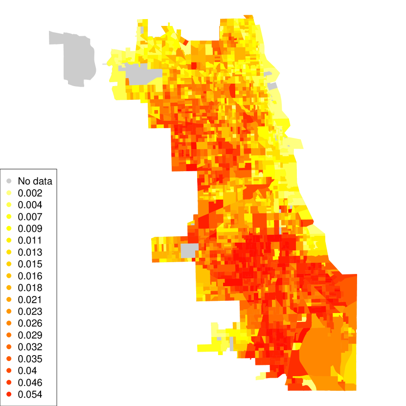
Figure 1: Observed proportions of reported burglaries per household between 2005–2009 in Chicago, IL. Data were aggregated within the 2010 census block groups.

Figure 2: A solution, corresponding to $\lambda=0.037$, along the graph fused lasso path that was fit to the observed proportions of burglaries.

We consider the task of estimating burglarly probabilities across Chicago census blocks, and simultaneously grouping or clustering these estimates across adjacent census blocks. The fused lasso, with an $\ell_{1}$ penalty on the differences between neighboring blocks, provides a means of carrying out this task. Using an $\ell_{2}$ or Huber penalty on the block differences would be easier for optimization, but would not be appropriate for the goal at hand because these smooth penalties are not capable of producing exact fusions in the components of the estimate. The fused lasso setup for the Chicago crime data used $n=2167$ blocks in total (nodes in the underlying graph), and $m=14,060$ connections between neighboring blocks (edges in the graph). Setting $X=I$, we computed the first 2500 steps of the fused lasso path, using the specialized implementation of Section 4, which took a little over a minute on a laptop computer. The largest degrees of freedom achieved by a solution in these first 2500 steps was 34.

Figure 2 displays one particular fused lasso solution from this path, corresponding to 8 degrees of freedom (Appendix E displays other solutions). Note that this solution divides the city into roughly four regions, with the most risky region being the southern side of the city, and the least risky being the northern side. In addition to the four main regions, we can also see that a small region of the city with very low burglary risk scores is isolated in the lower left part of the city; since it is buffered by a corridor of census blocks with no data, the region incurs only a small penalty for breaking off from the main graph. This picture in Figure 2 offers a better qualitative understanding of large scale spatial patterns than do the raw data in Figure 1. It also provides a high level clustering of census blocks which could be useful for police dispatchers, city planners, politicians, and insurance companies.

Lastly, we remark that one benefit of the fused lasso over many competing graph clustering methods is its local adaptivity. Simply put, the algorithm will adaptively determine the size of a cluster given the nodewise measurements, counter to the tendency of other methods in creating roughly equal sized clusters.

7 Empirical timings

Table 1 presented the theoretical per-iteration complexities of the various specialized implementations of the generalized lasso path algorithm. Here we briefly explore the empirical scaling of our implementations. For many classes of generalized lasso problems, as the problem size $n$ grows, the number of iterations taken by the path algorithm before termination can increase super-linearly in $n$. (A notable exception is the 1d fused lasso problem with $X=I$, in which the number of iterations before termination is always $n-1$.) For large problems, therefore, solving the entire path becomes computationally infeasible, and also often undesirable (typically, applications call for the more regularized solutions visited toward the start of the path). Hence, we investigate the time required to compute the first $100$ iterations of the path algorithm; continuing further down the path should scale accordingly with the number of steps.

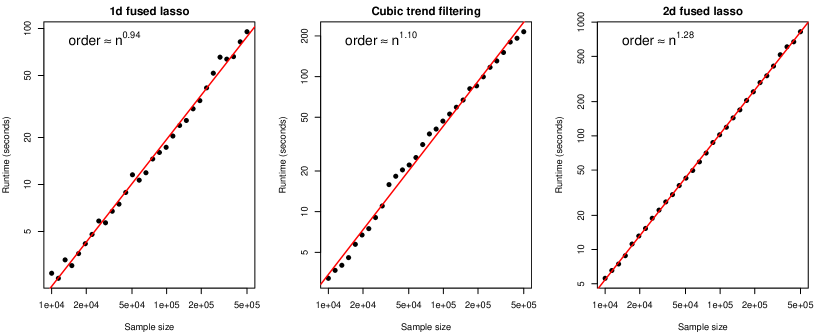
Figure 3: Runtimes from computing the first 100 steps of the generalized lasso path for 30 problem sizes ranging from $n=1000$ to $n=50,000$. The left panel shows the results for 1d fused lasso problems, the middle shows cubic trend filtering problems, and the right shows 2d fused lasso problems. Each plot is on a log-log scale, and a least squares line (passing through 0) was fit to determine the empirical scaling of each implementation with $n$.

The runtimes for the first $100$ path steps, with the sample size $n$ varying from $1000$ to $50,000$, are presented in Figure 3. These were timed on a laptop computer. We considered three problem classes, all with $X=I$: the 1d fused lasso, cubic trend filtering, and the 2d fused lasso problem classes. For the first two settings, we generated noisy observations around a mean following a two-period sinusoidal function. For the 2d fused lasso setting, we generated noisy observations over an approximately square grid, around a mean that was elevated in the bottom third quadrant of the grid. Note that the empirical complexity of the first 100 steps, in both the 1d fused lasso and trend filtering settings, is approximately linear, as predicted by the theoretical analysis. The steps in the 2d fused lasso computation scales slightly slower, but still not far from linear.

Across all three settings, our empirically derived scalings indicate that 100 path steps can be computed for problem sizes into the millions within a relatively short (i.e., less than one hour) time period. This bodes well for the 1d fused lasso and trend filtering problems, because in these cases, hundreds or thousands of path steps can often deliver regularized solutions of interest, even in very large problem sizes. However, for the 2d fused lasso problem, it is more often the case that many, many steps are needed to deliver solutions of interest. This has to do the connectivity of the graph corresponding to $D_{-\mathcal{B}}$, with $\mathcal{B}$ being the boundary set—see Section 4.2, or Tibshirani & Taylor (2011). We have found that the number of steps needed for interesting solutions scales more favorably when running the fused lasso on a graph determined by geographic regions (e.g., census block groups, as in Sections 6), but the number of steps grows prohibitively large for grid graphs, especially in a setting like image denoising, where the desired solutions often display a large number of connected components and hence require many steps.

Finally, we note that these runtimes were calculated using a default version of R (specifically, R version 3.1). As our specialized implementations all use built-in R matrix functions in one way or another, compiling R against a commercial matrix library will likely improve these results drastically on multicore machines.

8 Discussion

We have developed efficient implementations of the generalized lasso dual path algorithm of Tibshirani & Taylor (2011). In particular, we derived an implementation for a general penalty matrix $D$, one for trend filtering problems, in which $D$ is the discrete difference operator of a given order, and one for fused lasso problems, in which $D$ is the oriented incidence matrix of some underlying graph. Each implementation can handle the signal approximator case, $X=I$, as well as a general predictor matrix $X$. These implementations are all put to use in the genlasso R package.

Appendix A The QR decomposition and least squares problems

Here we give a brief review of the QR decomposition, and the application of this decomposition to least squares problems. Chapter 5 of Golub & Van Loan (1996) is an excellent reference.

A.1 The QR decomposition of a full column rank matrix

Let $A\in\mathbb{R}^{m\times n}$ with $\mathrm{rank}(A)=n$ (this implies that $m\geq n$). Then there exists matrices $Q\in\mathbb{R}^{m\times m}$ and $R\in\mathbb{R}^{m\times n}$ such that $A=QR$, where $Q$ is orthogonal (its first $n$ columns form a basis for the column space of $A$), and $R$ is of the form

$$R=\left[\begin{array}[]{c}R_{1}\\ 0\end{array}\right],$$

$R_{1}\in\mathbb{R}^{n\times n}$ being upper triangular. This is (not surprisingly) called the QR decomposition, and it can be computed in $O(mn^{2})$ operations (Golub & Van Loan, 1996).

The decomposition $A=QR$ is used primarily for solving least squares problems. For example, given $b\in\mathbb{R}^{m}$, suppose that are interested in finding $x\in\mathbb{R}^{n}$ to minimize

$$\|b-Ax\|_{2}^{2}.$$ (27)

Since $\mathrm{rank}(A)=n$, the minimizer $x$—also referred to as the solution—is unique. Let $Q_{1}\in\mathbb{R}^{m\times n}$ denote the first $n$ columns of $Q$, and let $Q_{2}\in\mathbb{R}^{m\times(m-n)}$ denote the last $m-n$ columns. Then

$$\|b-Ax\|_{2}^{2}=\|Q^{T}(b-Ax)\|_{2}^{2}=\|Q_{1}^{T}b-R_{1}x\|_{2}^{2}+\|Q_{2}^{T}b\|_{2}^{2},$$

and so minimizing the left-hand side is equivalent to minimizing $\|Q_{1}^{T}b-R_{1}x\|_{2}^{2}$. This can be done quickly, by solving the equation $R_{1}x=c$ where $c=Q_{1}^{T}b$. Recalling the triangular structure of $R_{1}$, this looks like:

$$\left[\begin{array}[]{ccccc}\Box&\Box&\Box&\Box&\Box\\ &\Box&\Box&\Box&\Box\\ &&\Box&\Box&\Box\\ &&&\Box&\Box\\ &&&&\Box\end{array}\right]\cdot x=c,$$

where the boxes denote nonzero entries, and blank spaces indicate zero entries. We first solve the equation given by last row (an equation in one variable), then we substitute and solve the second to last row, etc. This back-solve procedure takes $O(n^{2})$ operations. Hence, finding the least squares solution of (27) requires $O(mn)+O(n^{2})=O(mn)$ operations in total (the first term counts the multiplication by $Q_{1}^{T}$ to form $c=Q_{1}^{T}b$). Note that this does not count the $O(mn^{2})$ operations required to compute the QR decomposition of $A$ in the first place; and importantly, if we want to minimize multiple criterions of the form (27) for different vectors $b$, then we only compute the QR decomposition of $A$ once, and use this decomposition to find each solution quickly in $O(mn)$ operations.

A.2 The QR decomposition of a column rank deficient matrix

Let $A\in\mathbb{R}^{m\times n}$ with $\mathrm{rank}(A)=k\leq n$. Then there exists $P\in\mathbb{R}^{n\times n}$, $Q\in\mathbb{R}^{m\times m}$, and $R\in\mathbb{R}^{m\times n}$ such that $AP=QR$, where $P$ is a permutation matrix, $Q$ is orthogonal (its first $k$ columns span the column space of $A$), and $R$ decomposes as

$$R=\left[\begin{array}[]{cc}R_{1}&R_{2}\\ 0&0\end{array}\right],$$

where $R_{1}\in\mathbb{R}^{k\times k}$ is upper triangular, and $R_{2}\in\mathbb{R}^{k\times(n-k)}$ is dense. Visually, $R$ looks like this (when the order of rank deficiency is $n-k=2$):

$$\left[\begin{array}[]{ccccc}\Box&\Box&\Box&\Box&\Box\\ &\Box&\Box&\Box&\Box\\ &&\Box&\Box&\Box\\ &&&{\color[rgb]{1,1,1}\Box}&{\color[rgb]{1,1,1}\Box}\\ &&&&{\color[rgb]{1,1,1}\Box}\end{array}\right].$$

Note that $AP$ just permutes the columns of $A$. This decomposition takes $O(mnk)$ operations (Golub & Van Loan, 1996).

The least squares criterion in (27) can now admit many solutions $x$ (in fact, infinitely many) if $\mathrm{rank}(A)<n$. If we simply want any solution $x$—Golub & Van Loan (1996) refer to this as a basic solution—then we can use the QR decomposition $AP=QR$. We write

$$\|b-Ax\|_{2}^{2} =\|b-APP^{T}x\|_{2}^{2}$$

$$=\|Q^{T}(b-APP^{T}x)\|_{2}^{2}$$

$$=\|Q_{1}^{T}b-\big{[}R_{1}\;\,R_{2}\big{]}P^{T}x\|_{2}^{2}+\|Q_{2}^{T}b\|_{2}^{2},$$

where $Q_{1}\in\mathbb{R}^{m\times k}$ contains the first $k$ columns of $Q$, and $Q_{2}\in\mathbb{R}^{m\times(m-k)}$ contains the last $m-k$ columns. We can now consider $z=P^{T}x$ as the optimization variable, and solve

$$\Big{[}\begin{array}[]{cc}R_{1}&R_{2}\end{array}\Big{]}\left[\begin{array}[]{c}z_{1}\\ z_{2}\end{array}\right]=Q_{1}^{T}b,$$ (28)

where we have decomposed $z=(z_{1},z_{2})$ with $z_{1}\in\mathbb{R}^{k}$ and $z_{2}\in\mathbb{R}^{n-k}$. Note that to solve (28), we can take $z_{2}=0$, and then back-solve to compute $z_{1}$ in $O(k^{2})$ operations. Letting $x=Pz$, we have hence computed a basic least squares solution in $O(mk)+O(k^{2})+O(n)=O(mn)$ operations.

A.3 The minimum $\ell_{2}$ norm least squares solution

Suppose again that $A\in\mathbb{R}^{m\times n}$ and $\mathrm{rank}(A)=k\leq n$. If we want to compute the unique solution $x^{*}$ that has the minimum $\ell_{2}$ norm across all least squares solutions $x$ in (27), then the strategy given in the last section does not necessarily work (in fact, it does not produce $x^{*}$ unless $R_{2}=0$). However, we can modify the QR decomposition $AP=QR$ from Section A.2 in order to compute $x^{*}$. For this, we need to apply Givens rotations to $R$. These are covered in the next section, but for now, the key message is that there exists an orthogonal transformation $G\in\mathbb{R}^{n\times n}$ such that

$$RG=\widetilde{R}=\left[\begin{array}[]{cc}0&\widetilde{R}_{1}\\ 0&0\end{array}\right],$$ (29)

where $\widetilde{R}_{1}\in\mathbb{R}^{k\times k}$ is upper triangular. Applying a single Givens rotation to (the columns of) $R$ takes $O(k)$ operations, and $G$ is composed of $k(n-k)$ of them, so forming $RG$ takes $O(k^{2}(n-k))$ operations. Hence the decomposition $APG=Q\widetilde{R}$ requires the same order of complexity, $O(mnk)+O(k^{2}(n-k))=O(mnk)$ operations in total.

Now we write

$$\|b-Ax\|_{2}^{2}=\|b-APGz\|_{2}^{2},$$

where $z=G^{T}P^{T}x$. Since $P,G$ are orthogonal, we have $\|x\|_{2}=\|z\|_{2}$, and therefore our problem is equivalent to finding the minimum $\ell_{2}$ norm minimizer $z^{*}$ of the right-hand side above. As before, we now utilize the QR decomposition, writing

$$\|b-APGz\|_{2}^{2}=\|Q^{T}(b-APGz)\|_{2}^{2}=\|Q_{1}^{T}b-\big{[}0\;\,\widetilde{R}_{1}\big{]}z\|_{2}^{2}+\|Q_{2}^{T}b\|_{2}^{2},$$

where $Q_{1}\in\mathbb{R}^{m\times k}$ and $Q_{2}\in\mathbb{R}^{m\times(m-k)}$ give, respectively, the first $k$ and the last $m-k$ columns of $Q$. Hence we seek the minimum $\ell_{2}$ norm solution of

$$\Big{[}\begin{array}[]{cc}0&\widetilde{R}_{1}\end{array}\Big{]}\left[\begin{array}[]{c}z_{1}\\ z_{2}\end{array}\right]=Q_{1}^{T}b,$$

where $z=(z_{1},z_{2})$ with $z_{1}\in\mathbb{R}^{(n-k)}$ and $z_{2}\in\mathbb{R}^{k}$. For $z^{*}$ to have minimum $\ell_{2}$ norm, we must have $z^{*}_{1}=0$. Then $z^{*}_{2}$ is given by back-solving, which takes $O(k^{2})$ operations. Finally, we let $x^{*}=PGz^{*}$, and count $O(mk)+O(k^{2})+O(n^{2})+O(n)=O(n\cdot\max\{m,n\})$ operations in total to compute the minimum $\ell_{2}$ norm least squares solution.

A.4 The minimum $\ell_{2}$ norm least squares solution and the transposed QR

Given $A\in\mathbb{R}^{m\times n}$ with $\mathrm{rank}(A)=k\leq n$, it can be advantageous in some problems to use a QR decomposition of $A^{T}$ instead of $A$. (For example, this is the case when we want to update the QR decomposition after $A$ has changed by one column; see Section D.2.) By what we just showed, we can compute a decomposition $A^{T}PG=Q\widetilde{R}$, where $P\in\mathbb{R}^{m\times m}$ is a permutation matrix, $G\in\mathbb{R}^{m\times m}$ is an orthogonal matrix of Givens rotations, $Q\in\mathbb{R}^{n\times n}$ is orthogonal, and $\widetilde{R}\in\mathbb{R}^{n\times m}$ is of the special form (29) with $\widetilde{R}_{1}\in\mathbb{R}^{k\times k}$ upper triangular, in $O(mnk)$ operations.

To find the minimum $\ell_{2}$ norm minimizer $x^{*}$ of (27), we can employ a similar strategy to that of Section A.3. Using the orthogonality of $P,G$, and the computed decomposition $G^{T}P^{T}A=\widetilde{R}^{T}Q^{T}$, we have

$$\|b-Ax\|_{2}^{2}=\|G^{T}P^{T}(b-Ax)\|_{2}^{2}=\|c_{1}-\big{[}\widetilde{R}_{1}^{T}\;\,0\big{]}z\|_{2}^{2}+\|c_{2}\|_{2}^{2},$$

where $z=Q^{T}x$, and $c_{1},c_{2}$ denote the first $k$, respectively last $m-k$ coordinates of $c=G^{T}P^{T}b$. As $Q$ is orthogonal, we have $\|x\|_{2}=\|z\|_{2}$, and hence it suffices to find the minimum $\ell_{2}$ norm minimizer $z^{*}$ of the right-hand side above. This is the same as finding the minimum $\ell_{2}$ norm solution of the linear equation

$$\Big{[}\begin{array}[]{cc}\widetilde{R}_{1}^{T}&0\end{array}\Big{]}\left[\begin{array}[]{c}z_{1}\\ z_{2}\end{array}\right]=c_{2},$$

where $z=(z_{1},z_{2})$ with $z_{1}\in\mathbb{R}^{k}$ and $z_{2}\in\mathbb{R}^{(n-k)}$. Therefore $z_{2}^{*}=0$, and $z_{1}^{*}$ can be computed by foward-solving (the same concept as back-solving, except we start with the first row), requiring $O(k^{2})$ operations. We finally take $x^{*}=Qz^{*}$. The total number of operations is $O(n)+O(m^{2})+O(k^{2})+O(nk)=O(m\cdot\max\{m,n\})$.

Appendix B Givens rotations

We describe Givens rotations, orthogonal transformations that help maintain (or create) maintain upper triangular structure. Givens rotations provide a way to efficiently update the QR decomposition of a given matrix after a row or column has been added or deleted. (They also provide a way to compute the QR decomposition in the first place.) Our explanation and notation here are based largely on Chapter 5 of Golub & Van Loan (1996).

B.1 Simple Givens rotations in two dimensions

The main idea behind a Givens rotation can be expressed by considering the $2\times 2$ rotation matrix

$$G=\left[\begin{array}[]{cc}c&s\\ -s&c\end{array}\right],$$

where $c=\cos\theta$ and $s=\sin\theta$, for some $\theta\in[0,2\pi]$. Multiplication by $G^{T}$ amounts to a counterclockwise rotation through an angle $\theta$; since it is a rotation matrix, $G$ is clearly orthogonal. Furthermore, given any vector $(a,b)\in\mathbb{R}^{2}$, we can choose $c,s$ (choose $\theta$) such that

$$G^{T}\left[\begin{array}[]{c}a\\ b\end{array}\right]=\left[\begin{array}[]{c}d\\ 0\end{array}\right],$$

for some $d\in\mathbb{R}$. This is simply rotating $(a,b)$ onto the first coordinate axis, and by inspection we see that we must take $c=a/\sqrt{a^{2}+b^{2}}$ and $s=-b/\sqrt{a^{2}+b^{2}}$. Note that, from the point of view of computational efficiency, we never have to compute $\theta$ (which would require inverse trigonometric functions).

B.2 Givens rotations in higher dimensions

The same idea extends naturally to higher dimensions. Consider the $n\times n$ Givens rotation matrix

$$G=\left[\begin{array}[]{cccccccc}1&0&\ldots&0&\ldots&0&\ldots&0\\ 0&1&\ldots&0&\ldots&0&\ldots&0\\ \vdots&&&&&&&\\ 0&0&\ldots&c&\ldots&s&\ldots&0\\ \vdots&&&&&&&\\ 0&0&\ldots&-s&\ldots&c&\ldots&0\\ \vdots&&&&&&&\\ 0&0&\ldots&0&\ldots&0&\ldots&1\\ \end{array}\right];$$

in other words, $G$ is the $n\times n$ identity matrix, except with four elements $G_{ii},G_{ij},G_{ji},G_{jj}$ replaced with the corresponding elements of the $2\times 2$ Givens rotation matrix. We will write $G=G(i,j)$ to emphasize the dependence on $i,j$. It is straightforward to check that $G$ is orthogonal. Applying $G^{T}$ to a vector $x\in\mathbb{R}^{n}$ only affects components $x_{i}$ and $x_{j}$, and leaves all other components untouched: with $z=G^{T}x$, we have

$$z_{k}=\begin{cases}cx_{i}-sx_{j}&\text{if}\;\,k=i\\ sx_{i}+cx_{j}&\text{if}\;\,k=j\\ x_{k}&\text{otherwise}\end{cases}.$$

Because $G^{T}$ only acts on two components, we can compute $z=G^{T}x$ in $O(1)$ operations. And as in the $2\times 2$ case, we can make $z_{j}=0$ by taking

$$c=x_{i}/\sqrt{x_{i}^{2}+x_{j}^{2}}\;\;\;\text{and}\;\;\;s=-x_{j}/\sqrt{x_{i}^{2}+x_{j}^{2}}.$$

Now we consider Givens rotations applied to matrices. If $A\in\mathbb{R}^{m\times n}$ and $G=G(i,j)\in\mathbb{R}^{m\times m}$, then pre-multiplying $A$ by $G^{T}$ (as in $G^{T}A$) only affects rows $i$ and $j$, and hence computing $G^{T}A$ takes $O(n)$ operations. Moreover, with the appropriate choice of $c,s$, we can selectively zero out an element in the $j$th row of $G^{T}A$. A common application of $G^{T}$ looks like the following:

$$G^{T}\cdot\left[\begin{array}[]{cccc}\Box&\Box&\Box&\Box\\ &\Box&\Box&\Box\\ &&\Box&\Box\\ &&\Box&\Box\\ &&&\Box\end{array}\right]=\left[\begin{array}[]{cccc}\Box&\Box&\Box&\Box\\ &\Box&\Box&\Box\\ &&\Box&\Box\\ &&&\Box\\ &&&\Box\end{array}\right],$$

where in this example $G=G(3,4)$, and $c,s$ have been chosen so that the element in the 4th row and 3rd column of the output is zero. Importantly, the first 2 columns of rows 3 and 4 were all zeros to begin with, and zeros after pre-multiplication, so that this zero pattern has not been disturbed (think of the $2\times 2$ case: rotating $(0,0)$ still gives $(0,0)$). Applying a second Givens rotation to the output gives an upper triangular structure:

$$G_{2}^{T}\cdot\left[\begin{array}[]{cccc}\Box&\Box&\Box&\Box\\ &\Box&\Box&\Box\\ &&\Box&\Box\\ &&&\Box\\ &&&\Box\end{array}\right]=\left[\begin{array}[]{cccc}\Box&\Box&\Box&\Box\\ &\Box&\Box&\Box\\ &&\Box&\Box\\ &&&\Box\\ &&&{\color[rgb]{1,1,1}\Box}\end{array}\right],$$

where $G_{2}=G_{2}(4,5)$ is another Givens rotation matrix.

On the other hand, post-multiplying $A\in\mathbb{R}^{m\times n}$ by a Givens rotation matrix $G=G(i,j)\in\mathbb{R}^{n\times n}$ (as in $AG$) only affects columns $i$ and $j$. Therefore computing $AG$ requires $O(m)$ operations. The logic is very similar to the pre-multiplication case, and by choosing $c,s$ appropriately, we can zero out a particular element in the $j$th column of $AG$. A common application looks like:

$$\left[\begin{array}[]{ccccc}\Box&\Box&\Box&\Box&\Box\\ &\Box&\Box&\Box&\Box\\ &&\Box&\Box&\Box\\ &&&&\Box\end{array}\right]\cdot G=\left[\begin{array}[]{ccccc}\Box&\Box&\Box&\Box&\Box\\ &\Box&\Box&\Box&\Box\\ &&&\Box&\Box\\ &&&&\Box\end{array}\right],$$

where $G=G(3,4)$ and $c,s$ were chosen to zero out the element in the 3rd row and 3rd column. Now applying two more Givens rotations yields an upper triangular structure:

$$\left[\begin{array}[]{ccccc}\Box&\Box&\Box&\Box&\Box\\ &\Box&\Box&\Box&\Box\\ &&&\Box&\Box\\ &&&&\Box\end{array}\right]\cdot G_{2}G_{3}=\left[\begin{array}[]{ccccc}{\color[rgb]{1,1,1}\Box}&\Box&\Box&\Box&\Box\\ &&\Box&\Box&\Box\\ &&&\Box&\Box\\ &&&&\Box\end{array}\right].$$

Appendix C Updating the QR decomposition in the full rank case

In this section we cover techniques based on Givens rotations for updating the QR decomposition of a matrix $A\in\mathbb{R}^{m\times n}$, after a row or column has been either added or removed to $A$. We assume here that $\mathrm{rank}(A)=n$; the next section covers the rank deficient case, which is more delicate. For the full rank update problem, a good reference is Section 12.5 of Golub & Van Loan (1996). Hence suppose that we have computed a decomposition $A=QR$, with $Q\in\mathbb{R}^{m\times m}$ and $R\in\mathbb{R}^{m\times n}$, as described in Section A.1, and we subsequently want to compute a QR decomposition of $\widetilde{A}$, where $\widetilde{A}$ differs from $A$ by either one row or one column. As motivation, we may have already solved the least squares problem

$$\|b-Ax\|_{2}^{2},$$

and now want to solve the new least squares problem

$$\|c-\widetilde{A}x\|_{2}^{2}.$$

As we will see, computing a QR decomposition of $\widetilde{A}$ by updating that of $A$ saves an order of magnitude in computational time when compared to the naive route (computing the QR decomposition “from scratch”). We treat the row and column update problems separately.

C.1 Adding or removing a row

Suppose that $\widetilde{A}\in\mathbb{R}^{(m+1)\times n}$ is formed by adding a row to $A$, following its $i$th row, so

$$A=\left[\begin{array}[]{c}A_{1}\\ A_{2}\end{array}\right]\;\;\;\text{and}\;\;\;\widetilde{A}=\left[\begin{array}[]{c}A_{1}\\ w^{T}\\ A_{2}\end{array}\right],$$

where $A_{1}\in\mathbb{R}^{i\times n}$, $A_{2}\in\mathbb{R}^{(m-i)\times n}$, and $w\in\mathbb{R}^{n}$ is the row to be added. Let $Q_{1}\in\mathbb{R}^{i\times m}$ denote the first $i$ rows of $Q$ and $Q_{2}\in\mathbb{R}^{(m-i)\times m}$ denote its last $m-i$ rows. By rearranging both the rows of $A$ the rows of $Q$ in the same way, the product $Q^{T}A$ remains the same:

$$\left[\begin{array}[]{cc}Q_{2}^{T}&Q_{1}^{T}\end{array}\right]\left[\begin{array}[]{c}A_{2}\\ A_{1}\end{array}\right]=Q^{T}A=R=\left[\begin{array}[]{c}R_{1}\\ 0\end{array}\right],$$

where $R_{1}\in\mathbb{R}^{n\times n}$ is upper triangular. Therefore

$$\left[\begin{array}[]{ccc}1&0&0\\ 0&Q_{2}^{T}&Q_{1}^{T}\end{array}\right]\left[\begin{array}[]{c}w^{T}\\ A_{2}\\ A_{1}\end{array}\right]=\left[\begin{array}[]{c}w^{T}\\ R_{1}\\ 0\end{array}\right].$$

We can now apply Givens rotations $G_{1},\ldots G_{n}$ so that

$$\widetilde{R}=G_{n}^{T}\ldots G_{1}^{T}\left[\begin{array}[]{c}w^{T}\\ R_{1}\\ 0\end{array}\right]=\left[\begin{array}[]{c}\widetilde{R}_{1}\\ 0\end{array}\right],$$

where $\widetilde{R}_{1}\in\mathbb{R}^{n\times n}$ is upper triangular. Hence defining

$$\widetilde{Q}=\left[\begin{array}[]{cc}0&Q_{1}\\ 1&0\\ 0&Q_{2}\end{array}\right]G_{1}\ldots G_{n},$$

and noting that $\widetilde{Q}\in\mathbb{R}^{(m+1)\times(m+1)}$ is still orthogonal, we have $\widetilde{A}=\widetilde{Q}\widetilde{R}$, the desired QR decomposition. This update procedure uses $n$ Givens rotations, and therefore it requires a total of $O(mn)$ operations. Compare this to the usual cost $O(mn^{2})$ of computing a QR decomposition (without updating).

On the other hand, suppose that $\widetilde{A}\in\mathbb{R}^{(m-1)\times n}$ is formed by removing the $i$th row of $A$. Hence

$$A=\left[\begin{array}[]{c}A_{1}\\ w^{T}\\ A_{2}\end{array}\right]\;\;\;\text{and}\;\;\;\widetilde{A}=\left[\begin{array}[]{c}A_{1}\\ A_{2}\end{array}\right],$$

where $A_{1}\in\mathbb{R}^{(i-1)\times n}$, $A_{2}\in\mathbb{R}^{(m-i)\times n}$, and $w\in\mathbb{R}^{n}$ is the row to be deleted. (We assume without a loss of generality that $m>n$, so that removing a row does not change the rank; updates in the rank deficient case are covered in the next section.) Let $q\in\mathbb{R}^{m}$ denote the $i$th row of $Q$, and note that we can compute Givens rotations $G_{1},\ldots G_{m-1}$ such that

$$G_{m-1}^{T}\ldots G_{1}^{T}q=se_{1},$$

with $e_{1}=(1,0,\ldots 0)\in\mathbb{R}^{m}$ the first standard basis vector, and $s=\pm 1$. Let $\widetilde{Q}=QG_{1}\ldots G_{m-1}$; then, as $\widetilde{Q}$ is still orthogonal, it has the form

$$\widetilde{Q}=\left[\begin{array}[]{cc}0&\widetilde{Q}_{1}\\ s&0\\ 0&\widetilde{Q}_{2}\end{array}\right],$$

where $\widetilde{Q}_{1}\in\mathbb{R}^{(i-1)\times(m-1)}$ and $\widetilde{Q}_{2}\in\mathbb{R}^{(m-i)\times(m-1)}$. Furthermore, defining $\widetilde{R}G_{m-1}^{T}\ldots G_{1}^{T}R$, we can see that

$$\widetilde{R}=\left[\begin{array}[]{c}v^{T}\\ \widetilde{R}_{1}\\ 0\end{array}\right],$$

where $\widetilde{R}_{1}\in\mathbb{R}^{n\times n}$ is upper triangular and $v\in\mathbb{R}^{n}$. By construction $A=QR=\widetilde{Q}\widetilde{R}$, and defining

$$\widetilde{Q}_{0}=\left[\begin{array}[]{c}\widetilde{Q}_{1}\\ \widetilde{Q}_{2}\end{array}\right]\;\;\;\text{and}\;\;\;\widetilde{R}_{0}=\left[\begin{array}[]{c}\widetilde{R}_{1}\\ 0\end{array}\right],$$

we have $\widetilde{A}=\widetilde{Q}_{0}\widetilde{R}_{0}$, as desired. We performed $m-1$ Givens rotations, and hence $O(m^{2})$ operations.

C.2 Adding or removing a column

Suppose that $\widetilde{A}\in\mathbb{R}^{m\times(n+1)}$ is formed by adding a column to $A$, say, after its $j$th column. Then

$$Q^{T}\widetilde{A}=\left[\begin{array}[]{ccc}R_{1}&\vdots&R_{2}\\ 0&w&R_{3}\vspace{-5pt}\\ 0&\vdots&0\end{array}\right],$$

where $R_{1}\in\mathbb{R}^{j\times j}$ and $R_{3}\in\mathbb{R}^{(n-j)\times(n-j)}$ are upper triangular, $R_{2}\in\mathbb{R}^{j\times(n-j)}$ is dense, and $w\in\mathbb{R}^{m}$. (We are assuming here, without a loss of generality, that the added column does not lie in the span of the existing ones; updates in the rank deficient case are covered in the next section.) We can apply Givens rotations $G_{1},\ldots G_{n-j}$ to the rows of $Q^{T}\widetilde{A}$ so that

$$G_{n-j}^{T}\ldots G_{1}^{T}Q^{T}\widetilde{A}=\left[\begin{array}[]{c}\widetilde{R}_{1}\\ 0\end{array}\right]=\widetilde{R},$$

where $\widetilde{R}_{1}\in\mathbb{R}^{(n+1)\times(n+1)}$ is upper triangular. Therefore with $\widetilde{Q}=QG_{1}\ldots G_{n-j}$, we have $\widetilde{A}=\widetilde{Q}\widetilde{R}$. We applied $O(n)$ Givens rotations, so this update procedure requires $O(mn)$ operations.

If instead $\widetilde{A}\in\mathbb{R}^{m\times(n-1)}$ is formed by removing the $j$th column of $A$, then

$$Q^{T}\widetilde{A}=\left[\begin{array}[]{cc}R_{1}&R_{2}\\ 0&w^{T}\\ 0&R_{3}\\ 0&0\end{array}\right],$$

where $R_{1}\in\mathbb{R}^{(j-1)\times(j-1)}$ and $R_{3}\in\mathbb{R}^{(n-j)\times(n-j)}$ are upper triangular, $R_{2}\in\mathbb{R}^{(j-1)\times(n-j)}$ is dense, and $w\in\mathbb{R}^{n-j}$. Note that we can apply Givens rotations $G_{1},\ldots G_{n-j}$ to the rows of $Q^{T}\widetilde{A}$ to produce

$$G_{n-j}^{T}\ldots G_{1}^{T}Q^{T}\widetilde{A}=\left[\begin{array}[]{cc}\widetilde{R}_{1}\\ 0\end{array}\right]=\widetilde{R},$$

where $\widetilde{R}_{1}\in\mathbb{R}^{(n-1)\times(n-1)}$ is upper triangular. Hence with $\widetilde{Q}=QG_{1}\ldots G_{n-j}$, we see that $\widetilde{A}=\widetilde{Q}\widetilde{R}$. Again we used $O(n)$ Givens rotations, and $O(mn)$ operations.

Appendix D Updating the QR decomposition in the rank deficient case

Here we again consider techniques for updating a QR decomposition, but study the more difficult case in which $A\in\mathbb{R}^{m\times n}$ with $\mathrm{rank}(A)=k\leq n$. In particular, we are interested in computing the minimum $\ell_{2}$ norm minimizer of

$$\|b-Ax\|_{2}^{2},$$ (30)

and subsequently, computing the minimum $\ell_{2}$ norm minimizer of

$$\|c-\widetilde{A}x\|_{2}^{2}.$$ (31)

where $\widetilde{A}$ has either one more or one less row that $A$, or else one more of one less column than $A$. Depending on whether whether our goal is to update the rows or columns, we actually need to use a different QR decomposition for the the initial least squares problem (30).

D.1 Adding or removing a row

We compute the minimum $\ell_{2}$ norm minimizer of the initial least squares criterion (30) using the QR decomposition $APG=QR$ described in Section A.3, where $P\in\mathbb{R}^{n\times n}$ is a permutation matrix, $G\in\mathbb{R}^{n\times n}$ is a product of Givens rotations matrices, $Q\in\mathbb{R}^{m\times m}$ and $R\in\mathbb{R}^{m\times n}$ is of the special form

$$R=\left[\begin{array}[]{cc}0&R_{1}\\ 0&0\end{array}\right],$$

with $R_{1}\in\mathbb{R}^{k\times k}$ upper triangular (we note, in order to avoid confusion, that $R,R_{1}$ were written as $\widetilde{R},\widetilde{R}_{1}$ in Section A.3).

First suppose that $\widetilde{A}\in\mathbb{R}^{(m+1)\times n}$ is formed by adding a row to $A$, after its $i$th row. Write

$$A=\left[\begin{array}[]{c}A_{1}\\ A_{2}\end{array}\right]\;\;\;\text{and}\;\;\;\widetilde{A}=\left[\begin{array}[]{c}A_{1}\\ w^{T}\\ A_{2}\end{array}\right],$$

where $A_{1}\in\mathbb{R}^{i\times n}$, $A_{2}\in\mathbb{R}^{(m-i)\times n}$, and $w\in\mathbb{R}^{n}$ is the row to be added. Also let $Q_{1}\in\mathbb{R}^{i\times m}$ and $Q_{2}\in\mathbb{R}^{(m-i)\times m}$ denote the first $i$ and last $m-i$ rows of $Q$, respectively. The logic at this step is similar to that in the full rank case: we can rearrange both the rows of $A$ and the rows of $Q$ so that the product $Q^{T}A$ will not change, hence

$$\left[\begin{array}[]{cc}Q_{2}^{T}&Q_{1}^{T}\end{array}\right]\left[\begin{array}[]{c}A_{2}\\ A_{1}\end{array}\right]PG=Q^{T}APG=R=\left[\begin{array}[]{cc}0&R_{1}\\ 0&0\end{array}\right].$$

Therefore

$$\left[\begin{array}[]{ccc}1&0&0\\ 0&Q_{2}^{T}&Q_{1}^{T}\end{array}\right]\left[\begin{array}[]{c}w^{T}\\ A_{2}\\ A_{1}\end{array}\right]PG=\left[\begin{array}[]{c}w^{T}PG\\ Q^{T}APG\end{array}\right]=\left[\begin{array}[]{cc}d_{1}^{T}&d_{2}^{T}\\ 0&R_{1}\\ 0&0\end{array}\right],$$ (32)

where $d_{1}\in\mathbb{R}^{n-k}$ and $d_{2}\in\mathbb{R}^{k}$ are the first $n-k$ and last $k$ components, respectively, of $d=G^{T}P^{T}w$. Now we must consider two cases. First, assume that $\mathrm{rank}(\widetilde{A})=\mathrm{rank}(A)$, so adding the new row to $A$ did not change its rank. This implies that $d_{1}=0$, and we can apply Givens rotations $G_{1},\ldots G_{k}$ to the right-hand side of (32) so that

$$\widetilde{R}=G_{k}^{T}\ldots G_{1}^{T}\left[\begin{array}[]{cc}0&d_{2}^{T}\\ 0&R_{1}\\ 0&0\end{array}\right]=\left[\begin{array}[]{cc}0&\widetilde{R}_{1}\\ 0&0\end{array}\right],$$

where $\widetilde{R}_{1}\in\mathbb{R}^{k\times k}$ is upper triangular. Letting

$$\widetilde{Q}=\left[\begin{array}[]{cc}0&Q_{1}\\ 1&0\\ 0&Q_{2}\end{array}\right]G_{1}\ldots G_{k},$$

we complete the desired decomposition $\widetilde{A}PG=\widetilde{Q}\widetilde{R}$. Note that this QR decomposition is of the appropriate form to compute the minimum $\ell_{2}$ norm solution of the least squares problem (31).

The second case to consider is $\mathrm{rank}(\widetilde{A})>\mathrm{rank}(A)$, which means that adding the new row to $A$ increased the rank. Then at least one component of $d_{1}$ is nonzero, and we can apply Givens rotations $G_{1},\ldots G_{n-k}$ to the right-hand side of (32) so that

$$\widetilde{R}=\left[\begin{array}[]{cc}d_{1}^{T}&d_{2}^{T}\\ 0&R_{1}\\ 0&0\end{array}\right]G_{1}\ldots G_{n-k}=\left[\begin{array}[]{cc}0&\widetilde{R}_{1}\\ 0&0\end{array}\right],$$

where $\widetilde{R}_{1}\in\mathbb{R}^{(k+1)\times(k+1)}$ is upper triangular. We let

$$\widetilde{Q}=\left[\begin{array}[]{cc}0&Q_{1}\\ 1&0\\ 0&Q_{2}\end{array}\right]\;\;\;\text{and}\;\;\;\widetilde{G}=GG_{1}\ldots G_{n-k},$$

and observe that $\widetilde{A}P\widetilde{G}=\widetilde{Q}\widetilde{R}$ is a QR decomposition of the desired form, so that we may compute the minimum $\ell_{2}$ norm minimizer of (31). Finally, in either case (an increase in rank or not), we used $O(n)$ Givens rotations, and so this update procedure requires $O(n\cdot\max\{m,n\})$ operations.

Alternatively, suppose that $\widetilde{A}\in\mathbb{R}^{(m-1)\times n}$ is formed by removing the $i$th row of $A$, so

$$A=\left[\begin{array}[]{c}A_{1}\\ w^{T}\\ A_{2}\end{array}\right]\;\;\;\text{and}\;\;\;\widetilde{A}=\left[\begin{array}[]{c}A_{1}\\ A_{2}\end{array}\right],$$

where $A_{1}\in\mathbb{R}^{(i-1)\times n}$, $A_{2}\in\mathbb{R}^{(m-i)\times n}$, and $w\in\mathbb{R}^{n}$ is the row to be deleted. We follow the same arguments as in the full rank case: we let $q\in\mathbb{R}^{m}$ denote the $i$th row of $Q$, and compute Givens rotations $G_{1},\ldots G_{m-1}$ such that

$$G_{m-1}^{T}\ldots G_{1}^{T}q=se_{1},$$

with $e_{1}=(1,0,\ldots 0)\in\mathbb{R}^{m}$ and $s=\pm 1$. Defining $\widetilde{Q}=QG_{1}\ldots G_{m-1}$, we see that

$$\widetilde{Q}=\left[\begin{array}[]{cc}0&\widetilde{Q}_{1}\\ s&0\\ 0&\widetilde{Q}_{2}\end{array}\right],$$

for $\widetilde{Q}_{1}\in\mathbb{R}^{(i-1)\times(m-1)}$ and $\widetilde{Q}_{2}\in\mathbb{R}^{(m-i)\times(m-1)}$, and defining $\widetilde{R}=G_{m-1}^{T}\ldots G_{1}^{T}R$, we have

$$\widetilde{R}=\left[\begin{array}[]{cc}v_{1}^{T}&v_{2}^{T}\\ 0&\widetilde{R}_{1}\\ 0&0\end{array}\right],$$

where $\widetilde{R}_{1}\in\mathbb{R}^{k\times k}$ has zeros below its diagonal, and $v_{1}\in\mathbb{R}^{n-k}$, $v_{2}\in\mathbb{R}^{k}$. As $APG=QR=\widetilde{Q}\widetilde{R}$, we let

$$\widetilde{Q}_{0}=\left[\begin{array}[]{c}\widetilde{Q}_{1}\\ \widetilde{Q}_{2}\end{array}\right]\;\;\;\text{and}\;\;\;\widetilde{R}_{0}=\left[\begin{array}[]{cc}0&\widetilde{R}_{1}\\ 0&0\end{array}\right],$$

and conclude that $\widetilde{A}PG=\widetilde{Q}_{0}\widetilde{R}_{0}$, which is almost the desired QR decomposition. We say almost because, if $\mathrm{rank}(\widetilde{A})<\mathrm{rank}(A)$ (removing the $i$th row decreased the rank), then the diagonal of $\widetilde{R}_{1}$ will have a zero element and hence it will not be upper triangular. If the $q$th diagonal element is zero, then we can perform Givens rotations $J_{1},\ldots J_{q-1}$ and $J_{q+1},\ldots J_{k}$ resulting in

$$\bar{R}_{0}=J_{q-1}^{T}\ldots J_{1}^{T}\widetilde{R}_{0}J_{q+1}\ldots J_{k}=\left[\begin{array}[]{cc}0&\bar{R}_{1}\\ 0&0\end{array}\right],$$

where $\bar{R}_{1}\in\mathbb{R}^{(k-1)\times(k-1)}$ is upper triangular. It helps to see a picture: with its 2nd diagonal element zero, $\widetilde{R}_{0}$ may look like

$$\left[\begin{array}[]{ccccc}{\color[rgb]{1,1,1}\Box}&\Box&\Box&\Box&\Box\\ &&&\Box&\Box\\ &&&\Box&\Box\\ &&&&\Box\\ &&&&{\color[rgb]{1,1,1}\Box}\end{array}\right],$$

so applying 2 Givens rotations to the rows,

$$J_{2}^{T}J_{1}^{T}\cdot\left[\begin{array}[]{ccccc}{\color[rgb]{1,1,1}\Box}&\Box&\Box&\Box&\Box\\ &&&\Box&\Box\\ &&&\Box&\Box\\ &&&&\Box\\ &&&&{\color[rgb]{1,1,1}\Box}\end{array}\right]=\left[\begin{array}[]{ccccc}{\color[rgb]{1,1,1}\Box}&\Box&\Box&\Box&\Box\\ &&&\Box&\Box\\ &&&&\Box\\ &&&&{\color[rgb]{1,1,1}\Box}\\ &&&&{\color[rgb]{1,1,1}\Box}\end{array}\right].$$

and a single Givens rotation to the columns,

$$\left[\begin{array}[]{ccccc}{\color[rgb]{1,1,1}\Box}&\Box&\Box&\Box&\Box\\ &&&\Box&\Box\\ &&&&\Box\\ &&&&{\color[rgb]{1,1,1}\Box}\\ &&&&{\color[rgb]{1,1,1}\Box}\end{array}\right]\cdot J_{4}=\left[\begin{array}[]{ccccc}{\color[rgb]{1,1,1}\Box}&{\color[rgb]{1,1,1}\Box}&\Box&\Box&\Box\\ &&&\Box&\Box\\ &&&&\Box\\ &&&&{\color[rgb]{1,1,1}\Box}\\ &&&&{\color[rgb]{1,1,1}\Box}\end{array}\right],$$

which has desired form. Letting $\bar{Q}_{0}=\widetilde{Q}_{0}J_{1}\ldots J_{q-1}$ and $\widetilde{G}=GJ_{q+1}\ldots J_{k}$, we have constructed the proper QR decomposition $\widetilde{A}P\widetilde{G}=\bar{Q}_{0}\bar{R}_{0}$. We used $O(m)$ Givens rotations, and $O(m\cdot\max\{m,n\})$ operations in total.

D.2 Adding or removing a column

If $\widetilde{A}$ has one more or less column than $A$, then one cannot obviously update the QR decomposition $APG=QR$ of $A$ to obtain such a decomposition for $\widetilde{A}$. Note that, if $\widetilde{A}$ differs from $A$ by one row, then $\widetilde{A}PG$ also differs from $APG$ by one row; but if $\widetilde{A}$ differs from $A$ by one column, then $\widetilde{A}$ does not even have the appropriate dimensions for post-multiplication by $PG$.

However, because adding or a removing a column to $A$ is the same as adding or removing a row to $A^{T}$, we can compute a QR decomposition $A^{T}PG=QR$, where now $P\in\mathbb{R}^{m\times m}$, $G\in\mathbb{R}^{m\times m}$, $Q\in\mathbb{R}^{n\times n}$, and $R\in\mathbb{R}^{n\times m}$, and update it using the strategies disussed in the previous section. The update procedure for addition requires $O(m\cdot\max\{m,n\})$ operations, and that for removal requires $O(n\cdot\max\{m,n\})$ operations. Hence, to be clear, we first compute the decomposition $A^{T}PG=QR$ in order to solve the initial least squares problem (30), as described in Section A.4, and then update it to form $\widetilde{A}^{T}\widetilde{P}\widetilde{G}=\widetilde{Q}\widetilde{R}$ (for some $\widetilde{P},\widetilde{G},\widetilde{Q},\widetilde{R}$), which we use to solve (31).

Appendix E More plots from the Chicago crime data example

The figures below display 5 more solutions along the fused lasso path fit to the Chicago crime data example, corresponding to 2, 5, 10, 15, and 25 degrees of freedom.

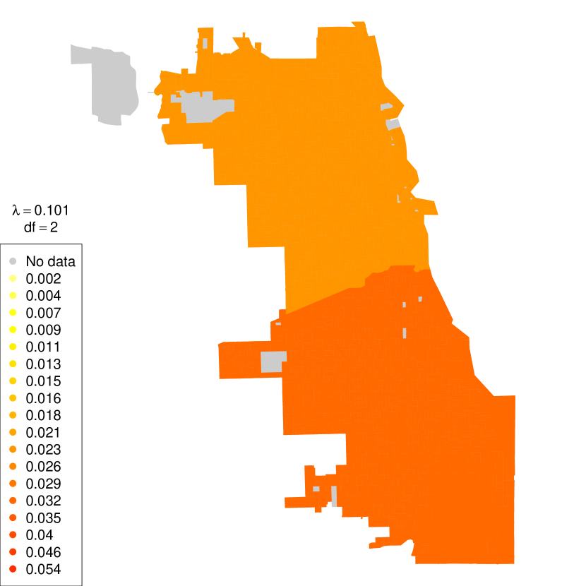
Figure 4: Fused lasso solution, from the Chicago crime data example, with $\lambda=0.101$.

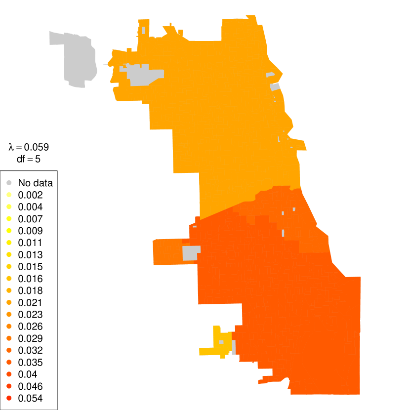
Figure 5: Fused lasso solution, from the Chicago crime data example, with $\lambda=0.059$.

Figure 6: Fused lasso solution, from the Chicago crime data example, with $\lambda=0.025$.

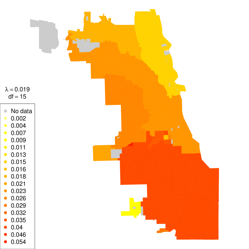
Figure 7: Fused lasso solution, from the Chicago crime data example, with $\lambda=0.019$.

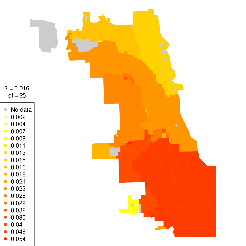
Figure 8: Fused lasso solution, from the Chicago crime data example, with $\lambda=0.016$.

References

- (1)
- Chambolle & Darbon (2009) Chambolle, A. & Darbon, J. (2009), ‘On total variation minimization and surface evolution using parametric maximum flows’, International Journal of Computer Vision 84, 288–307.
- Chen et al. (1998) Chen, S., Donoho, D. L. & Saunders, M. (1998), ‘Atomic decomposition for basis pursuit’, SIAM Journal on Scientific Computing 20(1), 33–61.
-
Chicago Police Department (2014)
Chicago Police Department (2014), ‘City of
chicago data portal, crimes – 2001 to present’.
https://data.cityofchicago.org/Public-Safety/Crimes-2001-to-present/ijzp-q8t2 - Davies & Kovac (2001) Davies, P. L. & Kovac, A. (2001), ‘Local extremes, runs, strings and multiresolution’, Annals of Statistics 29(1), 1–65.
- Davis (2011) Davis, T. (2011), ‘Algorithm 915, SuiteSparseQR: Multifrontal multithreaded rank-revealing sparse QR factorization’, ACM Transactions on Mathematical Software 38(1), 1–22.
- Davis & Hager (2009) Davis, T. & Hager, W. (2009), ‘Dynamic supernodes in sparse Cholesky update/downdate and triangular solves’, ACM Transactions on Mathematical Software 35(4), 1–23.
- Efron et al. (2004) Efron, B., Hastie, T., Johnstone, I. & Tibshirani, R. (2004), ‘Least angle regression’, Annals of Statistics 32(2), 407–499.
- Friedman et al. (2007) Friedman, J., Hastie, T., Hoefling, H. & Tibshirani, R. (2007), ‘Pathwise coordinate optimization’, Annals of Applied Statistics 1(2), 302–332.
- Golub & Van Loan (1996) Golub, G. H. & Van Loan, C. F. (1996), Matrix computations, The Johns Hopkins University Press, Baltimore. Third edition.
- Hoefling (2010) Hoefling, H. (2010), ‘A path algorithm for the fused lasso signal approximator’, Journal of Computational and Graphical Statistics 19(4), 984–1006.
- Johnson (2013) Johnson, N. (2013), ‘A dynamic programming algorithm for the fused lasso and -segmentation’, Journal of Computational and Graphical Statistics 22(2), 246–260.
- Kim et al. (2009) Kim, S.-J., Koh, K., Boyd, S. & Gorinevsky, D. (2009), ‘ trend filtering’, SIAM Review 51(2), 339–360.
- Land & Friedman (1996) Land, S. & Friedman, J. (1996), Variable fusion: a new adaptive signal regression method. http://www.stat.cmu.edu/tr/tr656/tr656.ps.
- Osborne et al. (2000a) Osborne, M., Presnell, B. & Turlach, B. (2000a), ‘A new approach to variable selection in least squares problems’, IMA Journal of Numerical Analysis 20(3), 389–404.
- Osborne et al. (2000b) Osborne, M., Presnell, B. & Turlach, B. (2000b), ‘On the lasso and its dual’, Journal of Computational and Graphical Statistics 9(2), 319–337.
-
R Development Core Team (2008)
R Development Core Team (2008), R: A
Language and Environment for Statistical Computing, R Foundation for
Statistical Computing, Vienna, Austria.
ISBN 3-900051-07-0.
http://www.R-project.org - Ramdas & Tibshirani (2014) Ramdas, A. & Tibshirani, R. (2014), Fast and flexible ADMM algorithms for trend filtering. arXiv: 1406.2082.
- Steidl et al. (2006) Steidl, G., Didas, S. & Neumann, J. (2006), ‘Splines in higher order TV regularization’, International Journal of Computer Vision 70(3), 214–255.
- Tibshirani (1996) Tibshirani, R. (1996), ‘Regression shrinkage and selection via the lasso’, Journal of the Royal Statistical Society: Series B 58(1), 267–288.
- Tibshirani (2014) Tibshirani, R. J. (2014), ‘Adaptive piecewise polynomial estimation via trend filtering’, Annals of Statistics 42(1), 285–323.
- Tibshirani & Taylor (2011) Tibshirani, R. J. & Taylor, J. (2011), ‘The solution path of the generalized lasso’, Annals of Statistics 39(3), 1335–1371.
- Tibshirani et al. (2005) Tibshirani, R., Saunders, M., Rosset, S., Zhu, J. & Knight, K. (2005), ‘Sparsity and smoothness via the fused lasso’, Journal of the Royal Statistical Society: Series B 67(1), 91–108.
- Vishnoi (2013) Vishnoi, N. (2013), ‘ – Laplacian solvers and their algorithmic applications’, Foundations and Trends in Theoretical Computer Science 8(1), 1–141.
- Zhou & Lange (2013) Zhou, H. & Lange, K. (2013), ‘A path algorithm for constrained estimation’, Journal of Computational and Graphical Statistics 22(2), 261–283.