On the Complexity of A/B Testing

Abstract

A/B testing refers to the task of determining the best option among two alternatives that yield random outcomes. We provide distribution-dependent lower bounds for the performance of A/B testing that improve over the results currently available both in the fixed-confidence (or $\delta$-PAC) and fixed-budget settings. When the distribution of the outcomes are Gaussian, we prove that the complexity of the fixed-confidence and fixed-budget settings are equivalent, and that uniform sampling of both alternatives is optimal only in the case of equal variances. In the common variance case, we also provide a stopping rule that terminates faster than existing fixed-confidence algorithms. In the case of Bernoulli distributions, we show that the complexity of fixed-budget setting is smaller than that of fixed-confidence setting and that uniform sampling of both alternatives—though not optimal—is advisable in practice when combined with an appropriate stopping criterion.

1 Introduction

A/B Testing is a popular procedure used, for instance, for website optimization: two versions of a webpage, say A and B, are empirically compared by being presented to users. Each user only sees one of the two versions, and the goal is to determine which version is preferable. We assume that the users provide a real-valued index of the quality of the pages, which is modeled by probability distributions $\nu_{A}$ and $\nu_{B}$, with respective means $\mu_{A}$ and $\mu_{B}$. For example, a standard objective is to determine which webpage has the highest conversion rate (probability that a user actually becomes a customer) by receiving binary feedback from the users.

Methods for A/B Testing are often viewed as statistical tests of the hypothesis $H_{0}:(\mu_{A}\leq\mu_{B})$ against $H_{1}:(\mu_{A}>\mu_{B})$. One may consider either classical tests, based on a number of samples $n_{A}$ and $n_{B}$ from each distribution fixed before the experiment, or sequential tests, based on paired samples ($X_{s},Y_{s}$) of $\nu_{A},\nu_{B}$ and in which a randomized stopping rule determines when the experiment is to be terminated. In both of these test settings, the sampling schedule is determined in advance, which is a possible source of sub-optimality as A/B Testing algorithms could take advantage of past observations to provide a smarter choice of the page to be displayed to the next user. In the sequel, we investigate whether A/B Testing could benefit from an adaptive sampling schedule. Ignoring the possible long-term effects on users of presenting one or the other option, we consider it as a particular instance of best arm identification in a two-armed bandit model.

A two-armed bandit model consists of two unknown probability distributions on $\mathbb{R}$, $\nu_{1}$ and $\nu_{2}$, sometimes referred to as arms or options (webpages in our motivating example). Arm $a$ has expectation $\mu_{a}$. At each time $t=1,2,\dots$, an agent chooses an option $A_{t}\in\{1,2\}$ and receives an independent draw $Z_{t}$ of the corresponding arm $\nu_{A_{t}}$. We denote by $\mathbb{P}_{\nu}$ (resp. $\mathbb{E}_{\nu}$) the probability law (resp. expectation) of the corresponding process $(Z_{t})$. We assume that the bandit model $\nu=(\nu_{1},\nu_{2})$ belongs to a class $\mathcal{M}$ such that for all $\nu\in\mathcal{M}$, $\mu_{1}\neq\mu_{2}$. In order to identify the best arm, that is the arm $a^{*}$ with highest expectation, the agent must use a strategy defining which arms to sample from, when to stop sampling, and which arm $\hat{a}$ to choose. The sampling rule determines how, at time $t$, the arm $A_{t}$ is chosen based on the past observations; in other words, $A_{t}$ is $\mathcal{F}_{t-1}$–measurable, with $\mathcal{F}_{t}=\sigma(A_{1},Z_{1},\dots,A_{t},Z_{t})$. The stopping rule $\tau$ is a stopping time with respect to $(\mathcal{F}_{t})_{t\in\mathbb{N}}$ satisfying $\mathbb{P}_{\nu}(\tau<+\infty)=1$. The recommendation rule is a $\mathcal{F}_{\tau}$-measurable random arm $\hat{a}\in\{1,2\}$. This triple $((A_{t}),\tau,\hat{a})$ entirely determines the strategy, which we denote in the sequel by $\mathcal{A}$. As discussed before, statistical tests correspond to strategies that sample the arms in a round-robin fashion, which we will refer to as uniform sampling.

In the bandit literature, two different settings have been considered. In the fixed-confidence setting, a risk parameter $\delta$ is fixed. A strategy $\mathcal{A}$ is called $\delta$-PAC if, for every choice of $\nu\in\mathcal{M}$, $\mathbb{P}_{\nu}(\hat{a}=a^{*})\geq 1-\delta$. The goal is, among the $\delta$-PAC strategies, to minimize the expected number of draws $\mathbb{E}_{\nu}[\tau]$. In the fixed-budget setting, the number of draws $\tau$ is fixed in advance ($\tau=t$ almost surely) and the goal is to choose the recommendation rule so as to minimize $p_{t}(\nu):=\mathbb{P}_{\nu}(\hat{a}\neq a^{*})$. In the fixed-budget setting, a strategy $\mathcal{A}$ is called consistent if, for every choice of $\nu\in\mathcal{M}$, $p_{t}(\nu)\underset{t\rightarrow\infty}{\rightarrow}0.$

In order to unify and compare these approaches, we define the complexity $\kappa_{C}(\nu)$ (resp. $\kappa_{B}(\nu)$) of best arm identification in the fixed-confidence (resp. fixed-budget) setting, as follows:

$$\kappa_{\text{C}}(\nu)=\inf_{\mathcal{A}\ \delta-\text{PAC}}\limsup_{\delta\rightarrow 0}\frac{\mathbb{E}_{\nu}[\tau]}{\log(1/\delta)},\hskip 28.45274pt\kappa_{\text{B}}(\nu)=\inf_{\mathcal{A}\ \text{consistent}}\left(\limsup_{t\rightarrow\infty}-\frac{1}{t}\log p_{t}(\nu)\right)^{-1}.$$

Heuristically, for a given bandit model $\nu$ and a given $\delta>0$, a fixed-confidence optimal strategy uses an average number of samples of order $\kappa_{C}(\nu)\log(1/\delta)$, whereas a fixed-budget optimal strategy uses approximately $t=\kappa_{B}(\nu)\log(1/\delta)$ draws in order to ensure a probability of error at most equal to $\delta$. Most of the existing performance bounds for the fixed confidence and fixed budget settings can be expressed using these complexity measures.

The main goal of this paper is to determine $\kappa_{\text{C}}$ and $\kappa_{\text{B}}$ for important classes of parametric bandit models, allowing for a comparison between the fixed-confidence and fixed-budget settings. Classical sequential testing theory provides a first element in that direction in the simpler case of fully specified alternatives. Consider for instance the case where $\nu_{1}$ and $\nu_{2}$ are Gaussian laws with the same known variance $\sigma^{2}$, the means $\mu_{1}$ and $\mu_{2}$ being known up to a permutation. Denoting by $P$ the joint distribution of the paired samples $(X_{s},Y_{s})$, one must choose between the hypotheses $H_{0}:P=\mathcal{N}\left(\mu_{1},\sigma^{2}\right)\otimes\mathcal{N}\left(\mu_{2},\sigma^{2}\right)$ and $H_{1}:P=\mathcal{N}\left(\mu_{2},\sigma^{2}\right)\otimes\mathcal{N}\left(\mu_{1},\sigma^{2}\right)$. It is known since [Wald (1945)] that among the sequential tests such that type I and type II probabilities of error are both smaller than $\delta$, the Sequential Probability Ratio Test (SPRT) minimizes the expected number of required samples, and is such that $\mathbb{E}_{\nu}[\tau]=2\sigma^{2}/(\mu_{1}-\mu_{2})^{2}\log(1/\delta)$. However, the batch test that minimizes both probabilities of error is the Likelihood Ratio test; it can be shown to require a sample size of order $8\sigma^{2}/(\mu_{1}-\mu_{2})^{2}\log(1/\delta)$ in order to ensure that both type I and type II error probabilities are smaller than $\delta$. Thus, when the sampling strategy is uniform and the parameters are known, there is a clear gain in using randomized stopping strategies. We show in the following that this conclusion is not valid anymore when the values of $\mu_{1}$ and $\mu_{2}$ are not assumed to be known.

Related works. Bandit models have received a considerable interest since their introduction by [Thompson (1933)]. An important focus was set on a different perspective, in which each observation is considered as a reward: the agent aims at maximizing the cumulative rewards obtained until some horizon $t$. Equivalently, his goal is to minimize the regret $R_{t}(\nu)=t\mu_{[1]}-\mathbb{E}_{\nu}\left[\sum_{s=1}^{t}Z_{s}\right]\;.$ Regret minimization, which is paradigmatic of the so-called exploration versus exploitation dilemma, was introduced by [Robbins (1952)] and its complexity is well understood for parametric bandits. In generic one-parameter models, [Lai and Robbins (1985)] prove that, with a proper notion of consistency adapted to regret minimization,

$$\inf_{A\ \text{consistent}}\liminf_{t\rightarrow\infty}\frac{R_{t}(\nu)}{\log t}\geq\sum_{a:\mu_{a}<\mu_{[1]}}\frac{(\mu_{[1]}-\mu_{a})}{\text{KL}(\nu_{a},\nu_{[1]})}\;,$$

where $\text{KL}(\nu_{i},\nu_{j})$ denotes the Kullback-Leibler divergence between distributions $\nu_{i}$ and $\nu_{j}$. Since then, non-asymptotic analyses of efficient algorithms matching this bound have been proposed. Optimal algorithms include the KL-UCB algorithm of [Cappé et al. (2013)]—a variant of UCB1 ([Auer et al. (2002)]) using informational upper bounds, Thompson Sampling ([Kaufmann et al. (2012b), Agrawal and Goyal (2013)]), the DMED algorithm (Honda and Takemura, 2011) and Bayes-UCB Kaufmann et al. (2012a). This paper is a first step in the attempt to similarly characterize the complexity of pure exploration, where the goal is to determine the best arms without trying to maximize the cumulated observations.

The problem of best arm identification has received an important interest in the 1950s as a particular case of ’ranking and identification problems’. The literature on the subject goes beyond two-armed bandit models to finding the $m>1$ best arms among $K>2$ arms, and sometimes introduces a relaxation parameter $\epsilon>0$, such that arms within $\epsilon$ of the best arm should be recommended. In the sequel, we always particularize the existing results to the two-armed bandit models presented above. The first advances on this topic are summarized in the monograph by Bechhofer et al. (1968), who only consider the fixed-confidence setting. In the same setting, algorithms introduced more recently by Even-Dar et al. (2006); Kalyanakrishnan et al. (2012); Gabillon et al. (2012) can be used to find the best arm in a two-armed bounded bandit model, in which $\nu_{1}$ and $\nu_{2}$ are probability distributions on $[0,1]$. Combining the upper bound on $\mathbb{E}_{\nu}[\tau]$ for the LUCB algorithm of Kalyanakrishnan et al. (2012) with the lower bound following from the work of Mannor and Tsitsiklis (2004), it can be shown that for bounded bandit models such that $\mu_{a}\in[0,1-\alpha]$ for $a\in\{1,2\}$, there exists a constant $C_{\alpha}$ for which

$${C_{\alpha}}/{(\mu_{1}-\mu_{2})^{2}}\leq\kappa_{C}(\nu)\leq{584}/(\mu_{1}-\mu_{2})^{2}.$$

The fixed-budget setting has been studied recently by Audibert et al. (2010); Bubeck et al. (2013). In two-armed bandit problems, the algorithms introduced in these papers boil down to sampling each arm $t/2$ times—$t$ denoting the total budget—and recommending the empirical best arm. A simple upper bound on the probability of error of this strategy can be derived, and this result paired with the lower bound of Audibert et al. (2010) yields, for bounded bandit models such that $\mu_{a}\in[\alpha;1-\alpha]$ for $a\in\{1,2\}$:

$${(2/5)\alpha(1-\alpha)}/{(\mu_{1}-\mu_{2})^{2}}\leq\kappa_{B}(\nu)\leq{2}/(\mu_{1}-\mu_{2})^{2}.$$

Bubeck et al. (2011) show that in the fixed-budget setting any sampling strategy designed to minimize regret performs poorly with respect to the simple regret $r_{t}:=\mu^{*}-\mu_{\hat{S}_{1}}$, a quantity closely related to the probability $p_{t}(\nu)$ of recommending the wrong arm. Therefore, good strategies for best arm identification have to be quite different from UCB-like strategies. We will show below that the complexities $\kappa_{B}(\nu)$ and $\kappa_{C}(\nu)$ of pure-exploration involve information terms that are different from the Kullback-Leibler divergence featured in Lai and Robbins’ lower bound on regret.

Contents of the paper. Compared to existing results, we provide general lower bounds on $\kappa_{B}(\nu)$ and $\kappa_{C}(\nu)$ that: (i) are tighter, leading in specific parametric cases to a precise evaluation of these complexities; (ii) do not require unnecessary support assumptions; and (iii) are stated in terms of information divergences between the distributions $\nu_{1}$ and $\nu_{2}$ rather than in terms of the gap $\mu_{1}-\mu_{2}$. As can be expected, we will indeed confirm that the inverse of the squared gap $(\mu_{1}-\mu_{2})^{2}$ is the relevant measure of complexity only in the Gaussian case, and an approximation (in the spirit of Pinsker’s inequality) for sub-Gaussian distributions.

Lower bounds on the sample complexity (resp. probability of error) of algorithms using the uniform sampling strategy in the fixed-confidence (resp. fixed-budget) setting are also derived and we show that for Gaussian bandit models with different variances, there is a significant gain in using a non-uniform sampling strategy. For Bernoulli bandits however, we show that little can be gained by departing from uniform sampling, and we therefore propose close-to-optimal tests both for the batch and sequential settings. For Gaussian bandits with a known common variance the optimal algorithm uses uniform sampling. In this specific case, we propose an improved $\delta$-PAC stopping rule, illustrating its performance through numerical experiments.

Our contributions follow from two main mathematical results: Lemma 6.1 provides a general relation between the expected number of draws and Kullback-Leibler divergences of the arms’ distributions, which is the key element to derive the lower bounds. Lemma 6.2 is a tight deviation inequality for martingales with sub-Gaussian increments, in the spirit of the Law of Iterated Logarithm.

The paper is structured as follows. Section 2 presents a distribution-dependent lower bound on both $\kappa_{B}(\nu)$ and $\kappa_{C}(\nu)$ under the some identifiability assumption, as well as lower bounds for algorithms using uniform sampling. Gaussian bandit models are then studied in details in Section 3, and Bernoulli bandit models in Section 4. Section 5 includes a practical illustration of the performance of matching algorithms for Gaussian bandits, as well as a practical comparison of the fixed-confidence and fixed-budget settings. The most important elements of proof are gathered in Section 6, with the rest of the proofs in the Appendix.

2 Lower Bounding the Complexity

Introducing the Kullback-Leibler divergence of any two probability distributions $p$ and $q$:

$$\mathrm{KL}(p,q)=\left\{\begin{array}[]{l}\int\log\left[\frac{dp}{dq}(x)\right]dp(x)\ \text{if}\ q\ll p,\\ +\infty\ \text{otherwise},\end{array}\right.$$

we make the assumption that there exists a set $\mathcal{N}$ such that for all $\nu=(\nu_{1},\nu_{2})\in\mathcal{M}$, for $a\in\{1,2\},\nu_{a}\in\mathcal{N}$ and that $\mathcal{N}$ satisfies

$$\forall p,q\in\mathcal{N},\ p\neq q\ \Rightarrow\ 0<\mathrm{KL}(p,q)<+\infty.$$

A class $\mathcal{M}$ of bandit models satisfying this property is called identifiable. For $\mathcal{M}$ an identifiable class of bandit models, Theorem 2.1 provides lower bounds on $\kappa_{B}(\nu)$ and $\kappa_{C}(\nu)$ for every $\nu\in\mathcal{M}$. The proof of this theorem is based on changes of distribution and detailed in Section 6.

Theorem 2.1.

Let $\mathbf{\nu}=(\nu_{1},\nu_{2})$ be a two-armed bandit model such that $\mu_{1}>\mu_{2}$. In the fixed-budget setting, any consistent algorithm satisfies

$$\limsup_{t\rightarrow\infty}-\frac{1}{t}\log p_{t}(\nu)\leq c^{*}(\nu),\ \ \ \text{where}\ \ \ c^{*}(\nu):=\inf_{(\nu_{1}^{\prime},\nu_{2}^{\prime})\in\mathcal{M}:\mu^{\prime}_{1}<\mu^{\prime}_{2}}\max\left\{\mathrm{KL}(\nu_{1}^{\prime},\nu_{1}),\mathrm{KL}(\nu_{2}^{\prime},\nu_{2})\right\}.$$

In the fixed-confidence setting any algorithm that is $\delta$-PAC on $\mathcal{M}$ satisfies, when $\delta\leq 0.15$,

$$\mathbb{E}_{\nu}[\tau]\geq\frac{1}{c_{*}(\nu)}\log\left(\frac{1}{2\delta}\right),\ \ \ \text{where}\ \ \ c_{*}(\nu):=\inf_{(\nu_{1}^{\prime},\nu_{2}^{\prime})\in\mathcal{M}:\mu_{1}^{\prime}<\mu_{2}^{\prime}}\max\left\{\mathrm{KL}(\nu_{1},\nu_{1}^{\prime}),\mathrm{KL}(\nu_{2},\nu_{2}^{\prime})\right\}.$$

In particular, Theorem 2.1 implies that $\kappa_{B}(\nu)\geq 1/{c^{*}(\nu)}$ and $\kappa_{C}(\nu)\geq 1/{c_{*}(\nu)}$. Proceeding similarly, one can obtain lower bounds for the algorithms that use uniform sampling of both arms. The proof of the following result is easily adapted from that of Theorem 2.1 (cf. Section 6), using that each arm is drawn $\tau/2$ times.

Theorem 2.2.

Let $\mathbf{\nu}=(\nu_{1},\nu_{2})$ be a two-armed bandit model such that $\mu_{1}>\mu_{2}$. In the fixed-budget setting, any consistent algorithm using a uniform sampling strategy satisfies

$$\limsup_{t\rightarrow\infty}-\frac{1}{t}\log p_{t}(\nu)\leq I^{*}(\nu)\ \ \ \text{where}\ \ \ I^{*}(\nu):=\inf_{(\nu_{1}^{\prime},\nu_{2}^{\prime})\in\mathcal{M}:\mu^{\prime}_{1}<\mu^{\prime}_{2}}\frac{\mathrm{KL}\left(\nu_{1}^{\prime},\nu_{1}\right)+\mathrm{KL}\left(\nu_{2}^{\prime},\nu_{2}\right)}{2}.$$

In the fixed-confidence setting, any algorithm that is $\delta$-PAC on $\mathcal{M}$ and uses a uniform sampling strategy satisfies, for $\delta\leq 0.15$,

$$\hskip 42.67912pt\mathbb{E}_{\nu}[\tau]\geq\frac{1}{I_{*}(\nu)}\log\frac{1}{2\delta}\ \ \ \text{where}\ \ \ I_{*}(\nu):=\inf_{(\nu_{1}^{\prime},\nu_{2}^{\prime})\in\mathcal{M}:\mu^{\prime}_{1}<\mu^{\prime}_{2}}\frac{\mathrm{KL}\left(\nu_{1},\nu_{1}^{\prime}\right)+\mathrm{KL}\left(\nu_{2},\nu_{2}^{\prime}\right)}{2}.$$

Obviously, one always has $I^{*}(\nu)\leq c^{*}(\nu)$ and $I_{*}(\nu)\leq c_{*}(\nu)$ suggesting that uniform sampling can be sub-optimal. It is possible to give explicit expressions for the quantities $c^{*}(\nu),c_{*}(\nu)$ and $I^{*}(\nu),I_{*}(\nu)$ for specific classes of parametric bandit models that will be considered in the rest of the paper. In the case of Gaussian bandits with known variance (see Section 3):

$$\mathcal{M}=\{\nu=\left(\mathcal{N}\left(\mu_{1},\sigma_{1}^{2}\right),\mathcal{N}\left(\mu_{2},\sigma_{2}^{2}\right)\right):(\mu_{1},\mu_{2})\in\mathbb{R}^{2},\mu_{1}\neq\mu_{2}\},$$ (1)

one obtains

$$c^{*}(\nu)=c_{*}(\nu)=\frac{(\mu_{1}-\mu_{2})^{2}}{2(\sigma_{1}+\sigma_{2})^{2}}\ \ \ \text{and}\ \ \ I^{*}(\nu)=I_{*}(\nu)=\frac{(\mu_{1}-\mu_{2})^{2}}{4(\sigma_{1}^{2}+\sigma_{2}^{2})}.$$

Hence, the lower bounds of Theorem 2.1 are equal in this case, and we provide in Section 3 matching upper bounds confirming that indeed $\kappa_{B}(\nu)=\kappa_{C}(\nu)$. In addition, the observation that $2I^{*}(\nu)\geq c^{*}(\nu)\geq I^{*}(\nu)$ implies that, except when $\sigma_{1}=\sigma_{2}$, strategies based on uniform sampling are sub-optimal.

The values of $c^{*}(\nu)$ and $c_{*}(\nu)$ can also be computed for canonical one-parameter exponential families with density with respect to some reference measure given by

$$f_{\theta}(x)=A(x)\exp(\theta x-b(\theta)),\ \ \text{for}\ \theta\in\Theta\subset\mathbb{R}.$$ (2)

We consider the class of bandit models

$$\mathcal{M}=\{\nu=(\nu_{\theta_{1}},\nu_{\theta_{2}}):(\theta_{1},\theta_{2})\in\Theta^{2},\theta_{1}\neq\theta_{2}\}$$

where $\nu_{\theta_{a}}$ has density $f_{\theta_{a}}$ given by (2). Using the shorthand $\mathrm{K}(\theta,\theta^{\prime})=\mathrm{KL}(\nu_{\theta},\nu_{\theta^{\prime}})$ for $(\theta,\theta^{\prime})\in\Theta^{2}$, one can show that, for $\nu$ such that $\mu_{1}>\mu_{2}$:

$$\begin{array}[]{ccccl}c^{*}(\nu)&=&\inf_{\theta\in\Theta}\max\left(\mathrm{K}(\theta,\theta_{1}),\mathrm{K}(\theta,\theta_{2})\right)&=&\mathrm{K}(\theta^{*},\theta_{1}),\ \ \text{where}\ \ \mathrm{K}(\theta^{*},\theta_{1})=\mathrm{K}(\theta^{*},\theta_{2}),\\ c_{*}(\nu)&=&\inf_{\theta\in\Theta}\max\left(\mathrm{K}(\theta_{1},\theta),\mathrm{K}(\theta_{2},\theta)\right)&=&\mathrm{K}(\theta_{1},\theta_{*}),\ \ \text{where}\ \ \mathrm{K}(\theta_{1},\theta_{*})=\mathrm{K}(\theta_{2},\theta_{*}).\end{array}$$

The coefficient $c^{*}(\nu)$ is known as the Chernoff information $\mathrm{K}^{*}(\theta_{1},\theta_{2})$ between the distributions $\nu_{\theta_{1}}$ and $\nu_{\theta_{2}}$ (see Cover and Thomas (2006) and Kaufmann and Kalyanakrishnan (2013) for earlier notice of the relevance of this quantity in the best arm selection problem). By analogy, we will also denote $c_{*}(\nu)$ by $\mathrm{K}_{*}(\theta_{1},\theta_{2})=\mathrm{K}(\theta_{1},\theta_{*})$.

For exponential family bandits the quantities $c^{*}(\nu)$ and $c_{*}(\nu)$ are not equal in general, although it can be shown that it is the case when the log-partition function $b(\theta)$ is (Fenchel) self-conjugate (e.g., for Gaussian and exponential variables). In Section 4, we will focus on the case of Bernoulli models for which $c^{*}(\nu)>c_{*}(\nu)$. By exhibiting a matching strategy in the fixed-budget case, we will show that this implies that $\kappa_{C}(\nu)>\kappa_{B}(\nu)$ in this case.

3 The Gaussian Case

We study in this Section the class of two-armed Gaussian bandit models with known variances defined by (1), where $\sigma_{1}$ and $\sigma_{2}$ are fixed. In this case, we observed above that the lower bounds of Theorem 2.1 are similar, because $c^{*}(\nu)=c_{*}(\nu)$. We prove in this section that indeed

$$\kappa_{C}(\nu)=\kappa_{B}(\nu)=\frac{2(\sigma_{1}+\sigma_{2})^{2}}{(\mu_{1}-\mu_{2})^{2}}$$

by exhibiting strategies that reach these performance bounds. These strategies are based on the simple recommendation of the empirical best arm but use non-uniform sampling in cases where $\sigma_{1}$ and $\sigma_{2}$ differ. When $\sigma_{1}=\sigma_{2}$ we provide in Theorem 3.1 an improved stopping rule that is $\delta$-PAC but results in a significant reduction of the running time of fixed-confidence tests.

3.1 Fixed-Budget Setting

We consider the simple family of static strategies that draw $n_{1}$ samples from arm 1 followed by $n_{2}=t-n_{1}$ samples of arm 2, and then choose arm 1 if $\hat{\mu}_{1,n_{1}}<\hat{\mu}_{2,n_{2}}$, where $\hat{\mu}_{i,n_{i}}$ denotes the empirical mean of the $n_{i}$ samples from arm $i$. Assume for instance that $\mu_{1}>\mu_{2}$. Since $\hat{\mu}_{1,n_{1}}-\hat{\mu}_{2,n_{2}}-\mu_{1}+\mu_{2}\sim\mathcal{N}\left(0,{\sigma_{1}^{2}}/{n_{1}}+{\sigma_{2}^{2}}/{n_{2}}\right)$, the probability of error of such a strategy is easily upper bounded as:

$$\mathbb{P}\left(\hat{\mu}_{1,n_{1}}<\hat{\mu}_{2,n_{2}}\right) \leq \exp\left(-\left(\frac{\sigma_{1}^{2}}{n_{1}}+\frac{\sigma_{2}^{2}}{n_{2}}\right)^{-1}\frac{(\mu_{1}-\mu_{2})^{2}}{2}\right).$$

The right hand side is minimized when $n_{1}/(n_{1}+n_{2})={\sigma_{1}}/{(\sigma_{1}+\sigma_{2})}$, and the static strategy drawing $n_{1}=\left\lceil\sigma_{1}t/(\sigma_{1}+\sigma_{2})\right\rceil$ times arm 1 is such that

$$\liminf_{t\rightarrow\infty}-\frac{1}{t}\log p_{t}(\nu)\geq\frac{(\mu_{1}-\mu_{2})^{2}}{2(\sigma_{1}+\sigma_{2})^{2}}\;,$$

which matches the bound of Theorem 2.1 for Gaussian bandit models.

3.2 Fixed-Confidence Setting

3.2.1 Equal Variances

We start with the simpler case $\sigma_{1}=\sigma_{2}=\sigma$, where the quantity $I_{*}(\nu)$ introduced in Theorem 2.2 coincides with $c_{*}(\nu)$, which suggests that uniform sampling could be optimal. A uniform sampling strategy is equivalent to collecting paired samples $(X_{s},Y_{s})$ from both arms. The difference $X_{s}-Y_{s}$ is Gaussian with mean $\mu=\mu_{1}-\mu_{2}$ and a $\delta$-PAC algorithm is equivalent to a sequential test of $H_{0}:\mu<0$ versus $H_{1}:\mu>0$ such that the probability of error is uniformly bounded by $\delta$. Robbins (1970) proposes such a test that stops after a number of samples

$$\tau=\inf\left\{t\in 2\mathbb{N}^{*}:\left|\sum_{s=1}^{t/2}(X_{s}-Y_{s})\right|>\sqrt{2\sigma^{2}t\beta(t,\delta)}\right\}\ \text{with}\ \beta(t,\delta)=\frac{t+1}{t}\log\left(\frac{t+1}{2\delta}\right)$$ (3)

and recommends the empirical best arm. This procedure belongs to the class of elimination strategies, introduced by Jennison et al. (1982) who derive a lower bound on the sample complexity of any $\delta$-PAC elimination strategy—whereas our lower bound applies to any $\delta$-PAC algorithm—matched by Robbins’ algorithm, that is, $\lim_{\delta\rightarrow 0}{\mathbb{E}_{\nu}[\tau]}/{\log\frac{1}{\delta}}={8\sigma^{2}}/{(\mu_{1}-\mu_{2})^{2}}.$ Therefore, Robbins’ rule (3) yields an optimal strategy matching our general lower bound of Theorem 2.1 in the particular case of Gaussian distributions with common known variance.

Note that any elimination strategy that is $\delta$-PAC and uses a threshold function smaller than Robbins’ also matches our asymptotic lower bound, while being strictly more efficient than Robbins’ rule. For practical purpose, it is therefore interesting to exhibit smaller exploration rates $\beta(t,\delta)$ leading to a $\delta$-PAC algorithm. The probability of error of such an algorithm is upper bounded, for example for $\mu_{1}<\mu_{2}$ by

$$\mathbb{P}_{\nu}\left(\exists k\in\mathbb{N}:\sum_{s=1}^{k}\frac{X_{s}-Y_{s}-(\mu_{1}-\mu_{2})}{\sqrt{2\sigma^{2}}}>\sqrt{2k\beta(2k,\delta)}\right)=\mathbb{P}\left(\exists k\in\mathbb{N}:S_{k}>\sqrt{2k\beta(2k,\delta)}\right)$$ (4)

where $S_{k}$ is a sum of $k$ i.i.d. variables of distribution $\mathcal{N}\left(0,1\right)$. Robbins (1970) obtains a non-explicit confidence region of risk at most $\delta$ by choosing $\beta(2k,\delta)=\log\left({\log(k)}/{\delta}\right)+o(\log\log(k))$. The dependency in $k$ is in some sense optimal, because the Law of Iterated Logarithm (LIL) states that $\limsup_{k\rightarrow\infty}{S_{k}}/\sqrt{2k\log\log(k)}=1$ almost surely. Recently, Jamieson et al. (2013) proposed an explicit confidence region inspired by the LIL. However, Lemma 1 of (Jamieson et al., 2013) cannot be used to upper bound (4) by $\delta$ and we provide in Section 6 a result derived independently (Lemma 6.2) that achieves this goal and yields the following result.

Theorem 3.1.

For $\delta$ small enough, the elimination strategy (3) is $\delta$-PAC with

$$\beta(t,\delta)=\log\frac{1}{\delta}+\frac{3}{4}\log\log\frac{1}{\delta}+\frac{3}{2}\log(1+\log(t/2)).$$ (5)

3.2.2 Mismatched Variances

In the case where $\sigma_{1}\neq\sigma_{2}$, we rely on an $\alpha$-elimination strategy, described in Algorithm 1. For $a=1,2$, $\hat{\mu}_{a}(t)$ denotes the empirical mean of the samples gathered from arm $a$ up to time $t$. The algorithm is based on a non-uniform sampling strategy governed by the parameter $\alpha\in(0,1)$ which ensures that, at the end of every round $t$, $N_{1}(t)=\lceil\alpha t\rceil$, $N_{2}(t)=t-\lceil\alpha t\rceil$ and $\hat{\mu}_{1}(t)-\hat{\mu}_{2}(t)\sim\mathcal{N}\left(\mu_{1}-\mu_{2},\sigma_{t}^{2}(\alpha)\right)$. The sampling schedule used here is thus deterministic.

Algorithm 1 $\alpha$-Elimination

0:  Exploration function $\beta(t,\delta)$, parameter $\alpha$.

1:  Initialization: $\hat{\mu}_{1}(0)=\hat{\mu}_{2}(0)=0$, $\sigma^{2}_{0}(\alpha)=1$. $t=0$.

2:  while $|\hat{\mu}_{1}(t)-\hat{\mu}_{2}(t)|\leq\sqrt{2\sigma^{2}_{t}(\alpha)\beta(t,\delta)}$ do

3:     $t=t+1$.

4:     If $\lceil\alpha t\rceil=\lceil\alpha(t-1)\rceil$, $A_{t}=2$, else $A_{t}=1$.

5:     Observe $Z_{t}\sim\nu_{A_{t}}$ and compute the empirical means $\hat{\mu}_{1}(t)$ and $\hat{\mu}_{2}(t)$.

6:     Compute $\sigma_{t}^{2}(\alpha)=\sigma_{1}^{2}/\lceil\alpha t\rceil+\sigma_{2}^{2}/(t-\lceil\alpha t\rceil).$

7:  end while

8:  return  $a=\underset{a=1,2}{\text{argmax}}\ \hat{\mu}_{a}(t)$

Theorem 3.2 shows that the $\sigma_{1}/(\sigma_{1}+\sigma_{2})$-elimination algorithm, with a suitable exploration rate, is $\delta$-PAC and matches the lower bound on $\mathbb{E}_{\nu}[\tau]$, at least asymptotically when $\delta\rightarrow 0$. Its proof can be found in Appendix LABEL:proof:MatchingFC.

Theorem 3.2.

If $\alpha=\sigma_{1}/(\sigma_{1}+\sigma_{2})$, the $\alpha$-elimination strategy using the exploration rate $\beta(t,\delta)=\log\frac{t}{\delta}+2\log\log(6t)$ is $\delta$-PAC on $\mathcal{M}$ and satisfies, for every $\nu\in\mathcal{M}$, for every $\epsilon>0$,

$$\mathbb{E}_{\nu}[\tau]\leq(1+\epsilon)\frac{2(\sigma_{1}+\sigma_{2})^{2}}{(\mu_{1}-\mu_{2})^{2}}\log\left(\frac{1}{\delta}\right)+\underset{\delta\rightarrow 0}{o_{\epsilon}}\left(\log\left(\frac{1}{\delta}\right)\right).$$

Remark 3.3.

When $\sigma_{1}=\sigma_{2}$, $1/2$-elimination reduces, up to rounding effects, to the elimination procedure described in Section 3.2.1, for which Theorem 3.1 suggests an exploration rate of order $\log(\log(t)/\delta)$. As the feasibility of this exploration rate when $\sigma_{1}\neq\sigma_{2}$ is yet to be established, we focus on Gaussian bandits with equal variances in the numerical experiments of Section 5.

4 The Bernoulli Case

We consider in this section the class of Bernoulli bandit models defined by

$$\mathcal{M}=\{\nu=\left(\mathcal{B}(\mu_{1}),\mathcal{B}(\mu_{2})\right):(\mu_{1},\mu_{2})\in]0;1[^{2},\mu_{1}\neq\mu_{2}\},$$

where each arm can be equivalently parametrized by the natural parameter of the exponential family, $\theta_{a}=\log({\mu_{a}}/{(1-\mu_{a})})$. Following the notation of Section 2, the Kullback-Leibler divergence between two Bernoulli distributions can be either expressed as a function of the means, $\mathrm{KL}(\mathcal{B}(\mu_{1}),\mathcal{B}(\mu_{2}))$, or of the natural parameters, $\mathrm{K}(\theta_{1},\theta_{2})$.

In this Section, we prove that $\kappa_{C}(\nu)>\kappa_{B}(\nu)$ for Bernoulli bandit models (Proposition 4.2). To do so, we first introduce a static strategy matching the lower bound of Theorem 2.1 in the fixed-budget case (Proposition 4.1). This strategy is reminiscent of the algorithm exhibited for Gaussian bandits in Section 3 and uses parameter-dependent non uniform sampling. This strategy is not directly helpful in practice but we show that it can be closely approximated by an algorithm using the uniform sampling strategy. In the fixed-confidence setting we similarly conjecture that little can be gained from using a non-uniform sampling strategy and propose an algorithm based on a non-trivial stopping strategy that is believed to match the bound of Theorem 2.2.

Proposition 4.1.

Let $\alpha(\theta_{1},\theta_{2})$ be defined by

$$\alpha(\theta_{1},\theta_{2})=\frac{\theta^{*}-\theta_{1}}{\theta_{2}-\theta_{1}}\ \ \ \text{where}\ \ \mathrm{K}(\theta^{*},\theta_{1})=\mathrm{K}(\theta^{*},\theta_{2}).$$

For all $t$, the static strategy that allocates $\left\lceil\alpha(\theta_{1},\theta_{2})t\right\rceil$ samples to arm 1 , and recommends the empirical best arm, satisfies $p_{t}(\nu)\leq\exp(-K^{*}(\theta_{1},\theta_{2})t)$.

This result, proved in Appendix LABEL:proof:ConcExp, shows in particular that for every $\nu\in\mathcal{M}$ there exists a consistent static strategy such that

$$\liminf_{t\rightarrow\infty}-\frac{1}{t}\log p_{t}\geq\mathrm{K}^{*}(\theta_{1},\theta_{2}),\ \ \ \text{andhencethat}\ \ \kappa_{B}(\nu)=\frac{1}{\mathrm{K}^{*}(\theta_{1},\theta_{2})}.$$

However, as $\alpha(\theta_{1},\theta_{2})$ depends in the Bernoulli case on the unknown means of the arms, this optimal static strategy is not useful in practice. So far, it is not known whether there exists a universal strategy such that $p_{t}(\nu)\leq\exp(-\mathrm{K}^{*}(\theta_{1},\theta_{2})t)$ for all bandit instance $\nu\in\mathcal{M}$.

For Bernoulli bandit models it can be checked that for all $\nu\in\mathcal{M}$, $\mathrm{K}_{*}(\theta_{1},\theta_{2})<\mathrm{K}^{*}(\theta_{1},\theta_{2})$. This fact together with Proposition 4.1 and Theorem 2.1 yields the following inequality.

Proposition 4.2.

For all $\nu\in\mathcal{M}$, $\kappa_{C}(\nu)>\kappa_{B}(\nu)$.

In the specific case of Bernoulli distributions, there is a strong incentive to use uniform sampling: the quantities $I^{*}(\nu)$ and $I_{*}(\nu)$ introduced in Theorem 2.2 appear to be very close to $c^{*}(\nu)$ and $c_{*}(\nu)$ respectively. This fact is illustrated in Figure 1, on which we represent these different quantities, that are functions of the means $\mu_{1},\mu_{2}$ of the arms, as a function of $\mu_{1}$, for two fixed values of $\mu_{2}$. Therefore, algorithms matching the bounds of Theorem 2.2 provide upper bounds on $\kappa_{B}(\nu)$ (resp. $\kappa_{C}(\nu)$) very close to $1/c^{*}(\nu)$ (resp. $1/c_{*}(\nu)$). In the fixed-budget setting, Lemma LABEL:lem:ConcExp shows that the strategy with uniform sampling that recommends the empirical best arm, satisfies $p_{t}(\nu)\leq e^{-tI^{*}(\nu)}$, and matches the bound of Theorem 2.2 (see Remark LABEL:rem:Match in Appendix LABEL:proof:ConcExp). Hence, problem-dependent optimal strategy described above can be approximated by a very simple, universal algorithm.

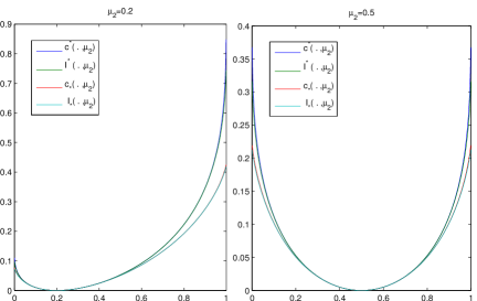
Figure 1: Comparison of different information terms in Bernoulli bandit models.

Similarly, finding an algorithm for the fixed-confidence setting sampling the arms uniformly and matching the bound of Theorem 2.2 is a crucial matter. This boils down to finding a good stopping rule. In all the algorithms studied so far, the stopping rule was based on the difference of the empirical means of the arms. For Bernoulli arms, such a strategy can be analyzed with the tools provided in this paper: the algorithm stopping for $t$ such that $\hat{\mu}_{1,t/2}-\hat{\mu}_{2,t/2}>\sqrt{{2\beta(t,\delta)}/{t}}$ with $\beta(t,\delta)$ as in Theorem 3.1 is $\delta$-PAC and its expected running time bounded by ${2}/{(\mu_{1}-\mu_{2})^{2}}\log\frac{1}{\delta}+o\left(\log\frac{1}{\delta}\right)$. Yet, Pinsker’s inequality implies that $I_{*}(\mu_{1},\mu_{2})>(\mu_{1}-\mu_{2})^{2}/2$ and this algorithm is thus not optimal with respect to Theorem 2.2. The approximation $I_{*}(\mu_{1},\mu_{2})=(\mu_{1}-\mu_{2})^{2}/(8\mu_{1}(1-\mu_{1}))+o\left((\mu_{1}-\mu_{2})^{2}\right)$ suggests that the loss with respect to the optimal error exponent is particularly significant when both means are close to 0 or 1. The stopping rule we propose to circumvent this drawback is the following:

$$\tau=\inf\left\{t\in 2\mathbb{N}^{*}:tI_{*}(\hat{\mu}_{1,t/2},\hat{\mu}_{2,t/2})>\log\left((\log(t)+1)/{\delta}\right)\right\}.$$ (6)

This algorithm is related to the KL-LUCB algorithm of Kaufmann and Kalyanakrishnan (2013). Indeed, $I_{*}(x,y)$ mostly coincides with $\mathrm{K}_{*}(\mathcal{B}(x),\mathcal{B}(y))$ (Figure 1) and a closer examination shows that the stopping criterion in KL-LUCB for two arms is exactly of the form $tK_{*}(\mathcal{B}(\hat{\mu}_{1,t/2}),\mathcal{B}(\hat{\mu}_{2,t/2}))>\beta(t,\delta)$. The results of Kaufmann and Kalyanakrishnan (2013) show in particular that the algorithm based on (6) is provably $\delta$-PAC for appropriate choices of $\beta(t,\delta)$. However, by analogy with the result of Theorem 3.1 we believe that the analysis of Kaufmann and Kalyanakrishnan (2013) is too conservative and that the proposed approach should be $\delta$-PAC for exploration rates $\beta(t,\delta)$ that grow as a function of $t$ only at rate $\log\log t$.

5 Numerical Experiments and Discussion

The goal of this Section is twofold: to compare results obtained in the fixed-budget and fixed-confidence settings and to illustrate the improvement resulting from the adoption of the reduced exploration rate of Theorem 3.1.

In Figure 2, we consider two bandit models: the ’easy’ one is $\mathcal{N}\left(0.5,0.25\right)\otimes\mathcal{N}\left(0,0.25\right)$, $\kappa=8$ (left) and the ’difficult’ one is $\mathcal{N}\left(0.01,0.25\right)\otimes\mathcal{N}\left(0,0.25\right)$, $\kappa=20000$ (right). In the fixed-budget setting, stars (’*’) report the probability of error $p_{n}(\nu)$ as a function of $n$. In the fixed-confidence setting, we plot both the empirical probability of error by circles (’O’) and the specified maximal error probability $\delta$ by crosses (’X’) as a function of the empirical average of the running times. Note the logarithmic scale used for the probabilities on the y-axis. All results are averaged on $N=10^{6}$ independent Monte Carlo replications. For comparison purposes, a plain line represents the theoretical rate $x\mapsto\exp(-x/\kappa)$ which is a straight line on the log scale.

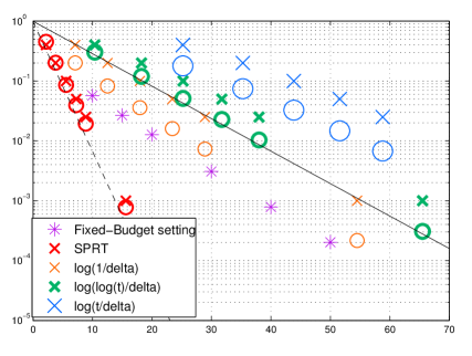
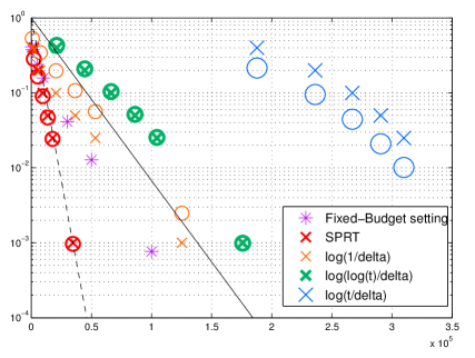
Figure 2: Experimental results (descriptions in text; plots best viewed in color).

In the fixed-confidence setting, we report results for algorithms of the form (3) with $g(t,\delta)=\sqrt{2\sigma^{2}t\beta(t,\delta)}$ for three different exploration rates $\beta(t,\delta)$. The exploration rate we consider are: the provably-PAC rate of Robbins’ algorithm $\log({t}/{\delta})$ (large blue symbols), the conjectured ’optimal’ exploration rate $\log({(\log(t)+1)}/{\delta})$, almost provably $\delta$-PAC according to Theorem 3.1 (bold green symbols), and the rate $\log({1}/{\delta})$, which would be appropriate if we were to perform the stopping test only at a single pre-specified time (orange symbols). For each algorithm, the log probability of error is approximately a linear function of the number of samples, with a slope close to $-1/\kappa$, where $\kappa$ is the complexity. We can visualize the gain in sample complexity achieved by smaller exploration rates, but while the rate $\log((\log(t)+1)/\delta)$ appears to guarantee the desired probability of error across all problems, the use of $\log(1/\delta)$ seems too risky, as one can see that the probability of error becomes larger than $\delta$ on difficult problems. To illustrate the gain in sample complexity when the means of the arms are known, we add in red the SPRT algorithm mentioned in the introduction along with the theoretical relation between the probability of error and the expected number of samples, materialized as a dashed line. The SPRT stops for $t$ such that $|(\mu_{1}-\mu_{2})(S_{1,t/2}-S_{2,t/2})|>\log(1/\delta)$.

Robbins’ algorithm is $\delta$-PAC and matches the complexity (which is illustrated by the slope of the measures), though in practice the use of the exploration rate $\log((\log(t)+1)/\delta)$ leads to huge gain in terms of number of samples used. It is important to keep in mind that running times play the same role as error exponents and hence the threefold increase of average running times observed on the rightmost plot of Figure 2 when using $\beta(t,\delta)=\log({t}/{\delta})$ is really prohibitive. This illustrates the asymptotic nature of our notion of complexity: the leading term in $\mathbb{E}_{\nu}[\tau]$ is indeed $\kappa\log(1/\delta)$ but there is a second-order constant term which is not negligible for fixed value of $\delta$. Jamieson et al. (2013) implicitly consider an alternative complexity for Gaussian bandit models with common known variance: for a fixed value of $\delta$, if $\Delta=\mu_{1}-\mu_{2}$, they show that when the gap $\Delta$ goes to zeros, the sample complexity if of order some constant—that depends on $\delta$—multiplied by $\Delta^{-2}\log\log\Delta^{-2}$.

If one compares on each problem the results for the fixed-budget setting to those for the best $\delta$-PAC algorithm (in green), one can see that to obtain the same probability of error, the fixed-confidence algorithm needs an average number of samples of order at least twice larger than the deterministic number of samples required by the fixed-budget setting algorithm. This remark should be related to the fact that a $\delta$-PAC algorithm is designed to be uniformly good across all problems, whereas consistency is a weak requirement in the fixed-budget setting: any strategy that draws both arm infinitely often and recommends the empirical best is consistent. Figure 2 shows that when the values of $\mu_{1}$ and $\mu_{2}$ are unknown, the sequential version of the test is no more preferable to its batch counterpart and can even become much worse if the exploration rate $\beta(t,\delta)$ is chosen too conservatively. This observation should be mitigated by the fact that the sequential (or fixed-confidence) approach is adaptive with respect to the difficulty of the problem whereas it is impossible to predict the efficiency of a batch (or fixed-budget) experiment without some prior knowledge regarding the problem under consideration.

6 Elements of Proof

6.1 Proof of Theorem 2.1

The cornerstone of the proof of all the lower bounds given in this paper is Lemma 6.1 which relates the probabilities of the same event under two different models to the expected number of draws of each arm. Its proof, which may be found in Appendix A, encapsulates the technical aspects of the change of distributions. $N_{a}(t)$ denotes the number of draws of arm $a$ up to round $t$ and $N_{a}=N_{a}(\tau)$ is the total number of draws of arm $a$ by some algorithm $\mathcal{A}$.

Lemma 6.1.

Let $\nu$ and $\nu^{\prime}$ be two bandit models. For any $A\in\mathcal{F}_{\tau}$ such that $0<\mathbb{P}_{\nu}(A)<1$

$$\mathbb{E}_{\nu}[N_{1}]\mathrm{KL}(\nu_{1},\nu^{\prime}_{1})+\mathbb{E}_{\nu}[N_{2}]\mathrm{KL}(\nu_{2},\nu^{\prime}_{2})\geq d(\mathbb{P}_{\nu}(A),\mathbb{P}_{\nu^{\prime}}(A)),$$ (7)

where $d(x,y):=\mathrm{KL}(\mathcal{B}(x),\mathcal{B}(y))=x\log(x/y)+(1-x)\log\big{(}(1-x)/(1-y)\big{)}.$

Without loss of generality, assume that the bandit model $\nu=(\nu_{1},\nu_{2})$ is such that $a^{*}=1$. Consider any alternative bandit model $\nu^{\prime}=(\nu_{1}^{\prime},\nu_{2}^{\prime})$ in which $a^{*}=2$ and the event $A=(\hat{a}=1)$ where $\hat{a}$ is the arm chosen by algorithm $\mathcal{A}$. Clearly $A\in\mathcal{F}_{\tau}.$

Fixed-Confidence Setting.

Let $\mathcal{A}$ be a $\delta$-PAC algorithm. Then it is correct on both $\nu$ and $\nu^{\prime}$ and satisfies $\mathbb{P}_{\nu}(A)\geq 1-\delta$ and $\mathbb{P}_{\nu^{\prime}}(A)\leq\delta$. Using monotonicity properties of $d$ (for example $x\mapsto d(x,y)$ is increasing when $x>y$ and decreasing when $x<y$) and inequality (7) in Lemma 6.1 yields $\mathbb{E}_{\nu}[N_{1}]\mathrm{KL}(\nu_{1},\nu_{1}^{\prime})+\mathbb{E}_{\nu}[N_{2}]\mathrm{KL}(\nu_{2},\nu_{2}^{\prime})\geq d(\delta,1-\delta)$, and hence

$$\mathbb{E}_{\nu}[\tau]\geq\frac{d(\delta,1-\delta)}{\max_{a=1,2}\mathrm{KL}(\nu_{a},\nu_{a}^{\prime})},$$

using that $\tau=N_{1}+N_{2}$. Optimizing over the possible model $\nu^{\prime}$ satisfying $\mu_{1}^{\prime}<\mu_{2}^{\prime}$ to make the right hand side of the inequality as large as possible gives the result, using moreover that for $\delta\leq 0.15$, it can be shown that $d(1-\delta,\delta)\geq\log({1}/(2\delta))$.

Fixed-Budget Setting.

Inequality (7) in Lemma 6.1 applied to $A$ yields

$$\mathbb{E}_{\nu^{\prime}}[N_{1}(t)]\mathrm{KL}(\nu^{\prime}_{1},\nu_{1})+\mathbb{E}_{\nu^{\prime}}[N_{2}(t)]\mathrm{KL}(\nu^{\prime}_{2},\nu_{2})\geq d(\mathbb{P}_{\nu^{\prime}}(A),\mathbb{P}_{\nu}(A)).$$

Note that $p_{t}(\nu)=1-\mathbb{P}_{\nu}(A)$ and $p_{t}(\nu^{\prime})=\mathbb{P}_{\nu^{\prime}}(A)$. As algorithm $\mathcal{A}$ is correct on both $\nu$ and $\nu^{\prime}$, for every $\epsilon>0$ there exists $t_{0}(\epsilon)$ such that for all $t\geq t_{0}(\epsilon)$, $\mathbb{P}_{\nu^{\prime}}(A)\leq\epsilon\leq\mathbb{P}_{\nu}(A)$. For $t\geq t_{0}(\epsilon)$,

$$\mathbb{E}_{\nu^{\prime}}[N_{1}(t)]\mathrm{KL}(\nu^{\prime}_{1},\nu_{1})+\mathbb{E}_{\nu^{\prime}}[N_{2}(t)]\mathrm{KL}(\nu^{\prime}_{2},\nu_{2})\geq d(\epsilon,1-p_{t}(\nu))\geq(1-\epsilon)\log\frac{1-\epsilon}{p_{t}(\nu)}+\epsilon\log{\epsilon}.$$

Taking the limsup (denoted by $\overline{\lim}$) and letting $\epsilon$ go to zero, one can show that

$$\overline{\lim}-\frac{1}{t}\log p_{t}(\nu) \leq \overline{\lim}\Bigl{[}\frac{\mathbb{E}_{\nu^{\prime}}[N_{1}(t)]}{t}\mathrm{KL}(\nu_{1}^{\prime},\nu_{1})+\frac{\mathbb{E}_{\nu^{\prime}}[N_{2}(t)]}{t}\mathrm{KL}(\nu_{2}^{\prime},\nu_{2})\Bigr{]}\leq\max_{a=1,2}\mathrm{KL}(\nu_{a}^{\prime},\nu_{a}).$$

Optimizing over the possible model $\nu^{\prime}$ satisfying $\mu_{1}^{\prime}<\mu_{2}^{\prime}$ to make the right hand side of the inequality as small as possible gives the result.

6.2 Proof of Theorem 3.1

According to (4), the proof of Theorem 3.1 boils down to finding an exploration rate such that $\mathbb{P}(\exists t\in\mathbb{N}^{*}:S_{t}>\sqrt{2\sigma^{2}t\beta(t,\delta)})\leq\delta$, where $S_{t}=X_{1}+\dots+X_{t}$ is a sum of i.i.d. normal random variable. Lemma 6.2 provides such a confidence region. Its proof can be found in Appendix LABEL:proof:DevIneq.

Lemma 6.2.

Let $\zeta(u)=\sum_{k\geq 1}k^{-u}$. Let $X_{1},X_{2},\dots$ be independent random variables such that, for all $\lambda\in\mathbb{R}$, $\phi(\lambda):=\log\mathbb{E}[\exp(\lambda X_{1})]\leq\lambda^{2}\sigma^{2}/2$. For every positive integer $t$ let $S_{t}=X_{1}+\dots+X_{t}$. Then, for all $\beta>1$ and $x\geq\frac{8}{(e-1)^{2}}$,

$$\mathbb{P}\Bigl{(}\exists t\in\mathbb{N}^{*}:{S_{t}}>\sqrt{2\sigma^{2}t(x+\beta\log\log(et))}\Bigr{)}\leq\sqrt{e}\,\zeta\Bigl{(}\beta\bigl{(}1-\frac{1}{2x}\bigr{)}\Bigr{)}\Bigl{(}\frac{\sqrt{x}}{2\sqrt{2}}+1\Bigr{)}^{\beta}\exp(-x).$$

Let $\beta(t,\delta)$ be of the form $\beta(t,\delta)=\log\frac{1}{\delta}+c\log\log\frac{1}{\delta}+d\log\log(et)$, for some constants $c>0$ and $d>1$. Lemma 6.2 yields

$$\mathbb{P}\Bigl{(}\exists t\in\mathbb{N}:S_{t}>\sqrt{2\sigma^{2}t\beta(t,\delta)}\Bigr{)}\leq\zeta\Bigl{(}d\bigl{(}1-\frac{1}{2(z+c\log z)}\bigr{)}\Bigr{)}\frac{\sqrt{e}}{(2\sqrt{2})^{d}}\frac{(\sqrt{z+c\log z}+\sqrt{8})^{d}}{z^{c}}\delta,$$

where $z:=\log\frac{1}{\delta}>0$. To upper bound the above probability by $\delta$, at least for large values of $z$ (which corresponds to small values of $\delta$), it suffices to choose the parameters $c$ and $d$ such that

$$\sqrt{e}\,\zeta\Bigl{(}d\bigl{(}1-\frac{1}{2(z+c\log z)}\bigr{)}\Bigr{)}\frac{1}{(2\sqrt{2})^{d}}\frac{(\sqrt{z+c\log z}+2\sqrt{2})^{d}}{z^{c}}\leq 1.$$

For $c={d}/{2}$, the left hand side tends to ${\sqrt{e}\zeta\left(d\right)}/{(2\sqrt{2})^{d}}$ when $z$ goes to infinity, which is smaller than 1 for $d\geq 1.47$. Thus, for $\delta$ small enough, the desired inequality holds for $d={3}/{2}$ and $c={3}/{4}$, which corresponds to the exploration rate of Theorem 3.1.

7 Conclusion

We provide distribution-dependent lower bounds for best-arm identification in the context of two-armed bandit models. These bounds involve information-theoretic quantities that reflect the typical causes of failure, which are different from those appearing in regret analysis. For Gaussian and Bernoulli bandit models, we exhibit matching algorithms showing that these bounds are (mostly) tight, highlighting relationships between the complexities of the fixed-budget and fixed-confidence settings. Our numerical experiments illustrate the significance of using appropriate exploration rates in the context of best arm(s) identification and we believe that Lemma 6.1 can be adapted to deal with more general $K$-armed bandit scenarios.

These results suggest three practical implications for A/B testing. First, for Binary and Gaussian-like responses with matched variances it is reasonable to consider only tests—i.e., strategies using uniform sampling—rather than general sequential sampling strategies. Second, using a sequential stopping rule in this context is mostly of interest because it does not requires prior knowledge of the complexity of the problem. It should however not be expected to reduce the (average) running time of the experiment for a given probability of error. This leads to the third message regarding the utmost importance of using proper (i.e., provably $\delta$-PAC but not too conservative) exploration rates when using a sequential stopping rule.

We thank Sébastien Bubeck for fruitful discussions during the visit of the first author at Princeton University. This work was supported by the ANR-2010-COSI-002 grant of the French National Research Agency.

Appendix A Proof of Lemma 6.1: Changes of Distributions

Under the identifiability assumption, there exists a common measure $\lambda$ such that for all $\nu=(\nu_{1},\nu_{2})$, for all $a\in\{1,2\}$ $\nu_{a}$ has a density $f_{a}$ with respect to $\lambda$.

Let $\nu\in\mathcal{M}$ be a bandit model, and consider an alternative bandit model $\nu^{\prime}\in\mathcal{M}$. $f_{a},f_{a}^{\prime}$ are the densities of $\nu_{a},\nu_{a}^{\prime}$ respectively and one can introduce the log-likelihood ratio of the observations up to time $t$ under an algorithm $\mathcal{A}$:

$$L_{t}:=\sum_{s=1}^{t}\mathds{1}_{(A_{s}=1)}\log\left(\frac{f_{1}(Z_{s})}{f^{\prime}_{1}(Z_{s})}\right)+\sum_{s=1}^{t}\mathds{1}_{(A_{s}=2)}\log\left(\frac{f_{2}(Z_{s})}{f^{\prime}_{2}(Z_{s})}\right).$$

The key element in a change of distribution is the following classical lemma (whose proof is omitted) that relates the probabilities of an event under $\mathbb{P}_{\nu}$ and $\mathbb{P}_{\nu^{\prime}}$ through the log-likelihood ratio of the observations. Such a result has often been used in the bandit literature for $\nu$ and $\nu^{\prime}$ that differ just from one arm (either $\nu_{1}=\nu^{\prime}_{1}$ or $\nu_{2}=\nu^{\prime}_{2}$), for which the expression of the log-likelihood ratio is simpler. As we will see, here we consider more general changes of distributions.

Lemma A.1.

Let $\sigma$ be any stopping time with respect to $\mathcal{F}_{t}$. For every event $A\in\mathcal{F}_{\sigma}$ (i.e. $A$ such that $A\cap(\sigma=t)\in\mathcal{F}_{t}$),

$$\mathbb{P}_{\nu^{\prime}}(A)=\mathbb{E}_{\nu}[\mathds{1}_{A}\exp(-L_{\sigma})]$$

Let $\tau$ be the stopping rule of algorithm $\mathcal{A}$. We start by showing that for all $A\in\mathcal{F}_{\tau}$, $\mathbb{P}_{\nu}(A)=0$ if and only if $\mathbb{P}_{\nu^{\prime}}(A)=0$. Thus, if $0<\mathbb{P}_{\nu}(A)<1$ one also has $0<\mathbb{P}_{\nu^{\prime}}(A)<1$ and the quantity $d(\mathbb{P}_{\nu}(A),\mathbb{P}_{\nu^{\prime}}(A))$ in the statement of Lemma 6.1 is well defined. Let $A\in\mathcal{F}_{\tau}$. Lemma A.1 yields $\mathbb{P}_{\nu^{\prime}}(A)=\mathbb{E}_{\nu}[\mathds{1}_{A}\exp(-L_{\tau})]$. Thus $\mathbb{P}_{\nu^{\prime}}(A)=0$ implies $\mathds{1}_{A}\exp(-L_{\tau})=0\ \mathbb{P}_{\nu}-a.s$. As $\mathbb{P}_{\nu}(\tau<+\infty)=1$, $\mathbb{P}_{\nu}(\exp(L_{\tau})>0)=1$ and $\mathbb{P}_{\nu^{\prime}}(A)=0\Rightarrow\mathbb{P}_{\nu}(A)=0$. A similar reasoning yields $\mathbb{P}_{\nu}(A)=0\Rightarrow\mathbb{P}_{\nu^{\prime}}(A)=0$.

We now prove Lemma 6.1. Let $A\in\mathcal{F}_{\tau}$ be such that $0<\mathbb{P}_{\nu}(A)<1$. Then $0<\mathbb{P}_{\nu^{\prime}}(A)<1$. Lemma A.1 and the conditional Jensen inequality leads to P_ν’(A) & = E_ν[exp(-L_τ)1_A] = E_ν[E_ν[exp(-L_τ) — 1_A] 1_A]
≥E_ν[exp

References

- Agrawal and Goyal (2013) S. Agrawal and N. Goyal. Further Optimal Regret Bounds for Thompson Sampling. In Conference on Artificial Intelligence and Statistics (AISTATS), 2013.
- Audibert et al. (2010) J-Y. Audibert, S. Bubeck, and R. Munos. Best Arm Identification in Multi-armed Bandits. In Conference on Learning Theory (COLT), 2010.
- Auer et al. (2002) P. Auer, N. Cesa-Bianchi, and P. Fischer. Finite-time analysis of the multiarmed bandit problem. Machine Learning, 47(2):235–256, 2002.
- Bechhofer et al. (1968) Robert Bechhofer, Jack Kiefer, and Milton Sobel. Sequential identification and ranking procedures. The university of Chicago Press, 1968.
- Bubeck et al. (2011) S. Bubeck, R. Munos, and G. Stoltz. Pure Exploration in Finitely Armed and Continuous Armed Bandits. Theoretical Computer Science, 412:1832–1852, 2011.
- Bubeck et al. (2013) S. Bubeck, T. Wang, and N. Viswanathan. Multiple Identifications in multi-armed bandits. In International Conference on Machine Learning (ICML), 2013.
- Cappé et al. (2013) O. Cappé, A. Garivier, O-A. Maillard, R. Munos, and G. Stoltz. Kullback-Leibler upper confidence bounds for optimal sequential allocation. Annals of Statistics, 41(3):1516–1541, 2013.
- Cover and Thomas (2006) T. Cover and J. Thomas. Elements of Information Theory (2nd Edition). Wiley, 2006.
- Even-Dar et al. (2006) E. Even-Dar, S. Mannor, and Y. Mansour. Action Elimination and Stopping Conditions for the Multi-Armed Bandit and Reinforcement Learning Problems. Journal of Machine Learning Research, 7:1079–1105, 2006.
- Gabillon et al. (2012) V. Gabillon, M. Ghavamzadeh, and A. Lazaric. Best Arm Identification: A Unified Approach to Fixed Budget and Fixed Confidence. In Neural Information and Signal Processing (NIPS), 2012.
- Honda and Takemura (2011) J. Honda and A. Takemura. An asymptotically optimal policy for finite support models in the multiarmed bandit problem. Machine Learning, 85(3):361–391, 2011.
- Jamieson et al. (2013) K. Jamieson, M. Malloy, R. Nowak, and S. Bubeck. lil’UCB: an optimal exploration algorithm for multi-armed bandits. arXiv:1312.7308, 2013.
- Jennison et al. (1982) C. Jennison, I.M. Johnstone, and B.W. Turnbull. Asymptotically optimal procedures for sequential adaptive selection of the best of several normal means. Statistical Decision Theory and Related Topics III, 2:55–86, 1982.
- Kalyanakrishnan et al. (2012) S. Kalyanakrishnan, A. Tewari, P. Auer, and P. Stone. PAC subset selection in stochastic multi-armed bandits. In International Conference on Machine Learning (ICML), 2012.
- Kaufmann and Kalyanakrishnan (2013) E. Kaufmann and S. Kalyanakrishnan. Information complexity in bandit subset selection. In Conference On Learning Theory (COLT), 2013.
- Kaufmann et al. (2012a) E. Kaufmann, A. Garivier, and O. Cappé. On Bayesian Upper-Confidence Bounds for Bandit Problems. In AISTATS, 2012a.
- Kaufmann et al. (2012b) E. Kaufmann, N. Korda, and R. Munos. Thompson Sampling : an Asymptotically Optimal Finite-Time Analysis. In Algorithmic Learning Theory (ALT), 2012b.
- Lai and Robbins (1985) T.L. Lai and H. Robbins. Asymptotically efficient adaptive allocation rules. Advances in Applied Mathematics, 6(1):4–22, 1985.
- Mannor and Tsitsiklis (2004) S. Mannor and J. Tsitsiklis. The Sample Complexity of Exploration in the Multi-Armed Bandit Problem. Journal of Machine Learning Research, pages 623–648, 2004.
- Robbins (1952) H. Robbins. Some aspects of the sequential design of experiments. Bulletin of the American Mathematical Society, 58(5):527–535, 1952.
- Robbins (1970) H. Robbins. Statistical Methods Related to the law of the iterated logarithm. Annals of Mathematical Statistics, 41(5):1397–1409, 1970.
- Siegmund (1985) D. Siegmund. Sequential Analysis. Springer-Verlag, 1985.
- Thompson (1933) W.R. Thompson. On the likelihood that one unknown probability exceeds another in view of the evidence of two samples. Biometrika, 25:285–294, 1933.
- Wald (1945) A. Wald. Sequential tests of statistical hypotheses. Annals of Mathematical Statistics, 16(2):117–186, 1945.