Dynamical formation of detached trans-Neptunian objects close to the 2:5 and 1:3 mean motion resonances with Neptune

Abstract

Aims. It is widely accepted that the past dynamical history of the solar system included a scattering of planetesimals from a primordial disk by the major planets. The primordial scattered population is likely the origin of the current scaterring disk and possibly the detached objects. In particular, an important argument has been presented for the case of $2004XR_{190}$ as having an origin in the primordial scattered disk through a mechanism including the 3:8 mean motion resonance (MMR) with Neptune (Gomes 2011). Here we aim at developing a similar study for the cases of the 1:3 and 2:5 resonances that are stronger than the 3:8 resonance.

Methods. Through a semi-analytic approach of the Kozai resonance inside a MMR, we show phase diagrams ($e,\omega$) that suggest the possibility of a scattered particle, after being captured in a mean motion resonance with Neptune, to become a detached object. We ran several numerical integrations with thousands of particles perturbed by the four major planets, and there are cases with and without Neptune’s residual migration. These were developed to check the semi-analytic approach and to better understand the dynamical mechanisms that produce the detached objects close to a MMR.

Results. The numerical simulations with and without a residual migration for Neptune stress the importance of a particular resonance mode, which we name the hibernating mode, on the formation of fossilized detached objects close to MMRs. When considering Neptune’s residual migration we are able to show the formation of detached orbits. These objects are fossilized and cannot be trapped in the MMRs again. We find a ratio of the number of fossilized objects with moderate perihelion distance ($35<q<40au$) to the number of objects with high perihelion distance ($q>40au$) as 3.0/1 for objects close to the 2:5, and 1.7/1 for objects close to the 1:3 resonance. We estimate that the two fossilized population have a total mass between $0.1$ and $0.3$ Pluto’s mass.

1 Introduction

Since the mid-twentieth century, scientists have speculated about the existence of small bodies beyond the orbit of Neptune (Edgeworth 1949; Kuiper 1951, 1974). These objects would form a disk and their orbits would have low eccentricities and inclinations. More than four decades later Jewitt & Luu (1993) found the first object, 1992QB₁, (except for Pluto and Charon) belonging to the Kuiper belt. This object’s orbital characteristics were consistent with those proposed by the first idealizers, with fairly low eccentricity and inclination. However, over the years, hundreds of new discoveries have revealed a much more complex scenario. One of the important unexplained features was the unexpectedly large number of objects with high inclinations. The first dynamical formation models (Malhotra 1993, 1995) were very successful at explaining several features of the Kuiper belt orbits, including the Plutinos and other resonant orbits, but in the end they failed to explain the high inclination of the Kuiper belt objects satisfactorily. Although up to now no theoretical model explain all the features of the trans-Neptunian region, the fact that there are many objects with high inclination orbits is something that differs a lot from what was initially expected. Gomes (2003a, b, 2011) have introduced, through a disk scattering mechanism, a new approach in producing high-inclination objects for the the hot population of the classical Kuiper belt and detached TNO’s.

The detached objects are roughly defined as having $a>50au$, $q\gtrsim 36au$, and usually high inclination ($i>10^{\circ}$). These characteristics provide much more stable dynamics without close encounters with Neptune, as is the case of the scattering disk objects whose perihelia, q, of the orbits approach Neptune ($30<q<35au$) and have semimajor axis $a>50au$. The detached population currently has the lowest number of discovered members, owing to the difficulty observing and tracking objects with large perihelia and high inclinations. But, detecting, tracking, and understanding how these objects could have formed may, nevertheless, reveal important dynamical processes that occurred in the primordial solar system (Gladman et al. 2002; Gomes et al. 2005b, 2008; Allen et al. 2006).

There have been several hypotheses for the dynamical formation of detached objects belonging to the detached group, since they started to be discovered. The object $2000CR_{105}$ ($a=228.8au,q=44.13au,i=22.77^{\circ}$) is one of the first discoveries belonging to the detached objects group, called “extended scattered disk” (ESD) at that time. Gladman et al. (2002) show that a process like long-term diffusive chaos is not good enough to reproduce such orbit. Then they propose other alternatives, such as perturbations by distant rogue planets or by primordial stellar passages as possible candidates to explain $2000CR_{105}$ dynamical formation. Gomes et al. (2006) show a mechanism for producing distant high-q detached objects, invoking the possibility that these bodies had interacted with a planetary-mass solar companion. Brasser et al. (2006, 2012), in turn, propose that the inner Oort cloud objects (actually, it is difficult to say when the detached population ends and the inner Oort cloud begins) would be formed by the perihelion-raising effect of a promordial cluster that was supposed to be the Sun’s birth environment. The authors consider close stellar encounters and the gas potential in the cluster as a scenario that produces such orbits with $a>200au$.

Gomes (2003a, b) and Gomes et al. (2005b) present a scenario where detached objects are generated exclusively through gravitational interaction with the Jovian planets. The authors propose that objects scattered during planetary migration can be captured in a mean motion resonance (MMR) with Neptune. Once in MMR, some particles could enter the Kozai resonance and present large variations in the eccentricities and inclinations. When the particle is in a low-eccentricity mode (and high inclination), the MMR critical angle may present a very large libration amplitude. Therefore, the object can escape both resonances while Neptune is still migrating, becoming a fossilized object with a high perihelion distance. Thus it is possible to produce detached orbits belonging to the ESD by just considering the perturbation of the giant planets, at least for $a\lesssim 100au$. To fossilize the orbits it is only necessary that Neptune experiences a residual migration. This mechanism could thus be valid in principle for both smooth migration (Hahn & Malhotra 1999, 2005) as well as for “direct emplacement” migration models (Tsiganis et al. 2005; Gomes et al. 2005a; Nesvorný 2011; Nesvorný & Morbidelli 2012).

Gomes (2011) uses this mechanism to explain the dynamical formation of $2004XR_{190}$ which is a fossilized object with high perihelion distance ($q\sim 51.6au$) and that is close to but not in the 3:8 MMR with Neptune (Allen et al. 2006). In his work the author highlights an interesting resonant mode in which the particle spends a long time with low eccentricity and high inclination (hibernating mode) and suggests that similar behavior should also occur for other MMRs. Although other models propose the formation of detached objects (Hahn & Malhotra 2005), we understand that the results in Gomes (2011) are compelling enough that we should reconsider the same mechanism applied to other important exterior MMRs with Neptune.

We thus intend to carry out a comprehensive study in this paper of the dynamical formation of detached objects near the 2:5 and 1:3 MMRs with Neptune, which are the strongest ones beyond the 1:2 MMR, since they have the smaller combination of order and degree. We performed several numerical integrations of the four giant planets and two disks of scattered particles surrounding the resonances of interest. We considered scenarios with the actual solar system and another one where Neptune is a little before its current position, so that one can impose a final phase of residual migration on Neptune. Therefore we intend to increase our understanding of the dynamical formation mechanism of detached objects near these MMRs.

The paper is divided as follows. In Section 2, we present the results of a many-particles numerical integration of the equations of motion of the major planets and a disk of planetesimals following the Nice model. This integration is used to determine the migration speed used in the following sections and also to present an example of the mechanism of creating fossilized detached objects that will motivate the rest of the work. In Section 3 we present a semi-analytic study of the Kozai mechanism inside the 2:5 and 1:3 MMRs. Section 4 shows the main results of our numerical experiments without Neptune’s residual migration. We devised a pathway for the formation of detached objects from primarily scattered particles, and relate it to the semi-analytic study developed in Section 3. Section 5 shows the main results of our numerical experiments with Neptune’s residual migration. We present a calculation of the ratio between detached objects with high and moderate perihelia and an estimate of the mass deposited near those resonances. Finally, we summarize our main results and give the conclusions in Section 6.

2 Results from a numerical integration with the Nice model

In this section we consider a numerical integration of the equations of motion of the planets and massive particles according to the Nice model (Tsiganis et al. 2005). The initial orbital semimajor axes for the planets are $5.45au$, $8.18au$, $11.5au$ and $14.2au$ for Jupiter, Saturn, Uranus, and Neptune, respectively. Their eccentricities are initially zero, and their inclinations are either $0^{\circ}$ or $0.5^{\circ}$. The disk is initially composed of $10^{3}$ planetesimals with a total mass of $35$ Earth masses, and with a surface density scaling as $r^{-1}$ and situated between $16.0$ and $40.0au$. They have zero eccentricities and inclinations. When the planets had stopped their mutual encounters, we cloned each planetesimal $30$ times. Figure 1 shows the evolution of the semimajor axes of the planets just before and after the instability phase triggered by the close encounters between the planets. We focus particularly on Neptune’s migration. Figure 2 shows the evolution of Neptune’s migration speed. This is done by averaging Neptune’s semimajor axes at every My, then averaging the migration speed taken from the previous averaged semimajor axes for every $100$ My. We notice that from $t=0.75$ Gy to $t=1.5$ Gy, Neptune’s migration speed varies roughly from $5au/Gy$ to $0.1au/Gy$. This is the range of speeds used in the simulations in Section 5, which corresponds to Neptune’s migration speed during a time span of roughly $0.85$ Gy. It must also be noticed that although after around $1.5$ Gy in the integration shown in Figure 2, Neptune has an average migration speed below $0.1au/Gy$ if we do not perform an average of these speeds. We notice the absolute value of Neptune’s migration speed above $0.1au/Gy$ during most of the time ($78$%). We might thus argue that in a sense Neptune has experienced a residual migration until today.

Figure 1: Evolution of semimajor axes of the giant planets for a Nice model simulation. Each planet in this plot is identified by its present order of distance from the Sun.

Figure 2: Evolution of Neptune’s migration speed during the Nice model simulation shown in Figure 1. Horizontal lines stand for migration speeds $0.1au/Gy$ and $0.5au/Gy$

This simulation also showed one instance of a trapping and later escape with respect to both the 2:5 and 1:3 resonances. Figure 3 shows such a case for the 2:5 resonance. We notice that a little after $0.8$ Gy to a little before $0.9$ Gy, the particle experiences the 2:5 MMR coupled with Kozai resonance. Somewhere before $0.9$ Gy, the particle escapes both resonances and gets apparently fossilized with fairly low eccentricity and high inclination. It is also instructive to follow the evolution of the resonant angle with more detail at two especific times of the particle’s evolution. This is shown in Figure 4 where in the lefthand panel the resonant angle is librating with $\sim 90^{\circ}$ amplitude around $180^{\circ}$. At around $0.884$ Gy (right panel), the particle’s resonant angle libation amplitude is very large and eventually turns to circulation, defining a escape from the resonance.

Figure 5 shows the distribution of the particle’s inclination around the 2:5 and 1:3 MMR, including a range of semimajor axes plus or minus $1au$ around the resonance’s nominal semimajor axis. The perihelion distances are from Neptune’s semimajor axis up to $5au$ beyond. These distributions will be useful for comparing with the simulations undertaken in the following sections. The data are from a time range between $0.7$ and $1$ Gy.

Figure 3: Orbital evolution of a SDO that get trapped into the 2:5 MMR with Neptune, experiences the Kozai mechanism and eventually escaped the resonance being fossilized as a detached object near the 2:5 resonance. Angles are in degrees.

Figure 4: Evolution of the 2:5 resonant angle for the same particle as in Figure 3 at two different times giving more detail on its variation. In the left panel, the particle is well inside the resonance. In the right panel the libration amplitude of the resonant angle is very large and eventually it switches to circulation. That would roughly define the time of escape from the resonance. Angles are in degrees.

Figure 5: Distribution of inclinations of particles around the 2:5 and 1:3 resonances. These inclinations were taken from a time range from $0.7$ to $1$ Gy in the Nice model simulation shown in Figure1.

3 A semi-analytic approach of the Kozai mechanism inside 2:5 and 1:3 MMRs

Based on the work of Thomas & Morbidelli (1996), Gomes et al. (2005b), Gomes (2011), and Gallardo et al. (2012), we developed our study for particles trapped in the 2:5 and 1:3 MMRs with Neptune. We consider the four major planets in planar and circular orbits. Our aim in this section is to find an average perturbation of the planets on the particle. This amounts to computing an average of the Hamiltonian in the mean longitudes of the planets and particle. When the particle experiences a MMR, the problem can be reduced to the calculation of a single integral, since we have a fixed relation between the mean longitudes of the planet and the particle given by the resonant angle (when its libration amplitude is zero). The general resonant angle is defined by

$$\qquad\qquad\qquad\phi=(p+q)\lambda_{N}-p\lambda-k_{1}\varpi-k_{2}\Omega$$ (1)

where $\lambda_{N}$ and $\lambda$ are the mean longitudes of Neptune and the particle, the integers $p$ and $q$ are the degree and order of the resonance, $k_{1},k_{2}$ are integers satisfying $k_{1}+k_{2}=q$, $\varpi$ is the particle’s longitude of perihelion and $\Omega$ its longitude of the ascending node. In the rest of the paper, we always consider $\phi_{2:5}$ and $\phi_{1:3}$ as the eccentricity-type ones, those that do not include the longitude of the node, defined by $\phi_{2:5}=5\lambda-2\lambda_{N}-3\varpi$ and $\phi_{1:3}=3\lambda-\lambda_{N}-2\varpi$.

In real N-body dynamics the particle always presents a finite libration amplitude of the resonant angle. Thus we turn back again to a double integral where the mean longitudes are still related through the resonant angle, which is made to vary according to a sinusoid of the given amplitude. Owing to the averaging in the particle’s mean longitude, its canonical conjugate

$$\qquad\qquad\qquad\qquad\qquad L=\sqrt{\mu a}$$ (2)

is constant. In Eq. (2), $a$ is the semimajor axis of the trans-Neptunian object and $\mu$ the gravitational constant times the Sun’s mass. Due to rotational invariance in the longitude of the node, its conjugate (divided by $L$)

$$\qquad\qquad\qquad\qquad H=\sqrt{1-e^{2}}\cos(i)$$ (3)

will also be a constant, where $i$ is the particle’s orbital inclination and $e$ its eccentricity. In the end, the averaged Hamiltonian will be in the form $E=E(G,g)$ where the canonical conjugated pair represents $g\equiv\omega$ (argument of perihelion), and $G=\sqrt{\mu a(1-e^{2})}$. Therefore, one has two constants of motion: the Hamiltonian ($E$), which is related to the energy, and $H$, which stands for the particle’s angular momentum projected on the reference (planets’ orbital) plane. Since our Hamiltonian is one degree of freedom, it is possible to draw level curves for fixed values of $E$ and $H$.

As pointed out by Kozai (1962), when the orbital inclination of the asteroid is high enough ($39^{\circ}\leq i\leq 141^{\circ}$ for asteroids in the main belt), its argument of perihelion starts to librate around fixed values ($\omega=k.90^{\circ}$, with $k$ an integer), and the pair ($e,i$) will be related by the constant of motion $H$. This kind of behavior has been known as Kozai resonance ever since then. Other authors have shown that if a TNO is trapped in a MMR with Neptune, it can present the Kozai dynamics for inclinations lower than $39^{\circ}$ (Gomes 2003a, b; Gomes et al. 2005b; Gomes 2011; Gallardo et al. 2012). Moreover, if the resonance is of type $1:N$, the classical Kozai centers vanish and new asymmetric centers ($\omega\neq k.90^{\circ}$) take their place (Kozai 1985; Gallardo et al. 2012). This is because the centers of $\phi_{1:N}$ are different from $0^{\circ}$ and $180^{\circ}$, and new terms in the mean resonant disturbing function arise (Gallardo et al. 2012).

From the semi-analytical approach described above we can build Figure 6, which shows two examples of diagrams e vs. $\omega$ for particles trapped in the 2:5 MMR. In figure 6(a) the particle has $H=0.851$, $a=55.47au$, $\bar{\phi}_{2:5}=180^{\circ}$, and $70^{\circ}$ of libration amplitude. Each level curve stands for a specific energy level and presents the classical Kozai dynamics where $\omega$ librates around the centers $\omega=k.90^{\circ}$. Therefore it is expected that a particle with these caracteristics presents anti-phase large variations in the pair ($e,i$) due to the conservation of $H$ and libration of $\omega$ around the classical centers. If the libration amplitude of $\phi_{2:5}$ increases, the relation between the mean longitudes is almost lost, and the motion will be similar to non-MMR Kozai dynamics. Figure 6(b) shows almost the same case as Figure 6(a), except that we now take $120^{\circ}$ for the libration amplitude of the resonant angle ($\phi_{2:5}$). Since $H$ is still a constant of motion, the lower curves represent orbits that have low eccentricities and high inclinations, while the higher ones have lower inclinations and higher eccentricities.

In Figure 7 we present a narrow window in time of one of our numerical simulations in which the process described above appears for a particle whose $H=0.851$. It experiences the 2:5 MMR coupled with the Kozai resonance for $\sim 100My$ ($\sim 3.27Gy$ to $\sim 3.37Gy$). Then it accesses a dynamical mode with low eccentricity or high perihelion distance (and high inclination) and high libration amplitude of the MMR angle for the rest of the simulation. We call this last dynamical mode of hibernating mode because the particle may “awake” at any time and return to the MMR+Kozai dynamics. In Figure 8 we show a zoom in time of Figure 7, for the unaveraged resonant angle. Although this behavior might be mistaken for a circulation, Figure 8 shows that the resonant angle is really librating when the libration period timescale is considered. On the other hand, the libration center is not constant but circulates. This is why it is more instructive to show the variation in the resonant angle in Figure 7 as averages in libration amplitude and libration center. It is important to note that in these exterior MMRs coupled with Kozai resonance, the variation of the libration center is the rule and not the exception.

Figure 9 presents the energy level curves associated with each square in Figure 7. The process of entering a hibernating mode seems quite subtle. In panel (c), the particle had a high libration amplitude, and the energy level curves were flat like in a non-MMR mode. In panel (d), the libration amplitude had already decreased enough to lead to the appearance of closed curves ($\omega$-librating) with large variations in the eccentricity. The particle thus manages to escape the hibernating mode along one of these Kozai curves. A similar process is observed from panels (g) to (h), but in this case the decrease of the libration amplitude was not large enough to create an ascending path for the particle, and as shown in panel (i), it enters the hibernating mode. The exact circumstances that enable a particle to enter or not the hibernating mode seems quite complicated and is most likely suitable to being studied as a probabilistic event, although that is beyond the scope of this paper. Owing the chaotic behavior of this dynamics, a particle once in hibernating mode can again be trapped in the MMR coupled with Kozai. To place the particle in a fossilized orbit, without the risk of being trapped again into the MMR, a complementar mechanism is needed. This will be discussed in the next sections.

Figure 6: (a) Energy level curves e vs. $\omega$ for a particle trapped in the 2:5 MMR, librating around $\bar{\phi}_{2:5}=180^{\circ}$ with $70^{\circ}$ of amplitude. We notice the appearance of the classical Kozai centers at $\omega=k.90^{\circ}$. The particle can experience large variations in the eccentricity and inclination. In (b) we have the same initial conditions as (a), except for the libration amplitude thas is now equal to $120^{\circ}$. We notice the disappearance of the classical Kozai centers at $\omega=k.90^{\circ}$. The large ($e,i$) variations are not possible, so each orbit will either have high eccentricity and low inclination or vice-versa.

Figure 7: Results of a numerical simulation in which the particle experiences the 2:5 MMR+Kozai, and the disappearance of both due to a large libration amplitude of $\phi_{2:5}$. The final orbit has low eccentricity, hence high inclination (not shown), because it is in a state called hibernating mode, since it can turn out to experience the MMR+Kozai due the chaotic behavior presented. The four panels show the time evolution of the eccentricity, argument of perihelion, mean resonant angle ($\phi_{2:5}$), and its amplitude, respectively. Angles are in degrees. The plotted squares stand for specific times for which energy level curves are plotted in Fig. 9.

Figure 8: The variation in the same resonant angle as in Figure 7 not averaged and zoomed in time so as to make the libration period timescale apparent. This behavior is common to exterior MMRs with Neptune coupled with Kozai resonance. Even when the particle is not in the hibernating mode, this behavior appears as, for instance, during the time between $3.3$ Gy and $3.32$ Gy as shown in Figure 7.

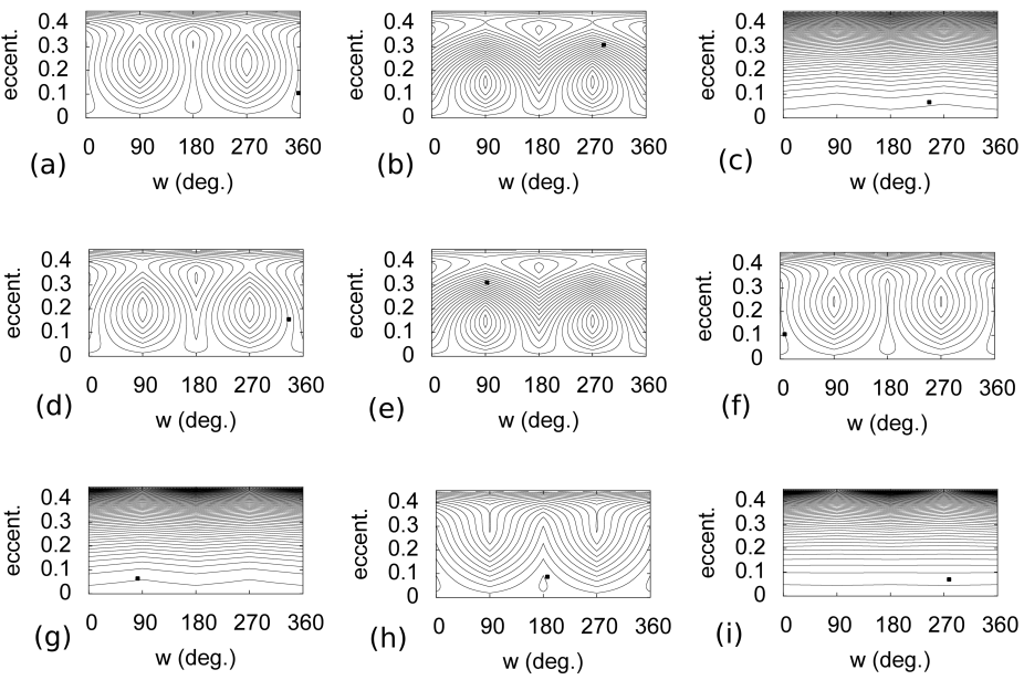
Figure 9: This sequence of shots are associated to the sequence of points in Figure 7 represented as squares. We plot $e$ vs. $\omega$ of the particle also as squares. At each point, the amplitude and libration center of the resonant angle enable us to plot the energy level curves associated with each square, so the squares follow equipotential curves in time-varying energy level diagrams. The main point is to show the random character of the entrance into the hibernating mode. Panels c and g are very similar and correspond to peaks in libration amplitude as shown in Figure 7. The transition to panels d and h shows the subtle difference between entering and not entering the hibernating mode.

For the 1:3 MMR, the same main features may occur, except that in this case when the inclination is high enough the asymmetric centers of the Kozai resonance appear. Figure 10 presents these asymmetric centers for different values of the libration center $\bar{\phi}_{1:3}$ and libration amplitudes. In all cases the particle preserves $a=62.63au$ and $H=0.82$. Again, if the amplitude of $\phi$ is large, the flattened curves appear, indicating that the hibernating mode is also possible for this resonance.

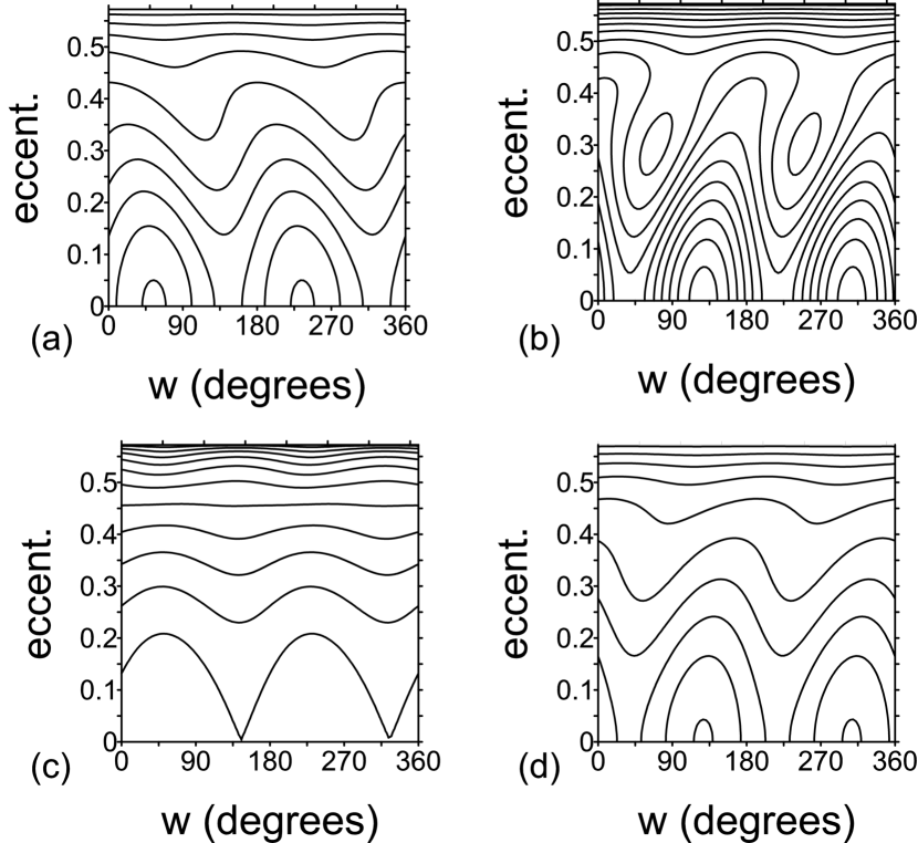
Figure 10: Energy level curves e vs. $\omega$ for the 1:3 MMR. In (a) $\bar{\phi}_{1:3}=70^{\circ}$ with $30^{\circ}$ of amplitude, in (b) $\bar{\phi}_{1:3}=285^{\circ}$ with $5^{\circ}$ of amplitude, in (c) $\bar{\phi}_{1:3}=70^{\circ}$ with $60^{\circ}$ of amplitude, and in (d) $\bar{\phi}_{1:3}=285^{\circ}$ with $30^{\circ}$ of amplitude. The asymmetric centers of the Kozai resonance are clear in (b), and the flattened curves in (c) indicate that the hibernating mode can also be reached. All cases have $a=62.63au$ and $H=0.82$.

4 Numerical simulations without migration

We present the results of seven numerical simulations of the equations of motion of the four giant planets in their current orbits referred to the ecliptic plane at Julian date 2454200.5 and a total of 22,500 massless scattered particles. The integrations were performed for $4.5Gy$ in steps of 0.5 years, which is approximately equal to 1/20 of the smallest orbital period (Jupiter). We used the hybrid integrator of the Mercury package (Chambers 1999) for these numerical simulations. The particles were divided into two groups around the mean motion resonances 2:5 ($a_{2:5}=55.5164au$) and 1:3 ($a_{1:3}=62.6912au$) with Neptune. Initial conditions were assigned randomly, respecting the following limits: $54.5161\leq a\leq 56.5161au$ or $61.6912\leq a\leq 63.6912au$ for semimajor axis, $30<q\leq 35au$ for perihelion distance, $0\leq i\leq 50^{\circ}$ for inclination, $[0,360^{\circ}]$ for the angles argument of perihelion $\omega$, longitude of the ascending node $\Omega$, and mean anomaly $l$. The planets interact among themselves and disturb the massless particles, which are discarded from the simulations when $a<52.50au$ or $a>65.75au$, decreasing the large cpu time spent to complete this kind of simulation. Since the particles are considered to be massless, there is no exchange of energy and angular momentum between the disks and the planets, and therefore there is no planetary migration.

We now present two representative figures that show the most interesting dynamic modes found. Figure 11 shows the case of a particle initially in the region of the 2:5 MMR, and in Figure 12 the particle was initially near the 1:3 MMR. The particle in Figure 11 starts in Kozai resonance and MMR, as seen in the middle and bottom plots and the coupled oscillation between the perihelion distance and inclination in the top plot. This Kozai mode, whose centers are $0$ and $180^{\circ}$, lasts about 700My. After that, the argument of perihelion starts to circulate with a long period, and the particle remains in a high-eccentricity orbit, whose perihelion is close to Neptune’s orbit, basically following similar dynamics to one of the top flattened curves of Figure 6-b, for $\sim 400My$. Close encounters with Neptune do not occur because it remains in MMR, as seen by the libration of $\phi_{2:5}$. Between $1.2Gy<t<3.4Gy$, the particle experiences a new type of Kozai mode, where the oscillations of eccentricity and inclination have greater amplitude and the libration centers of $\omega$ are most of the time at $90^{\circ}$ and $270^{\circ}$, but it circulates during some time around $2$ Gy. This behavior is also consistent with that shown in Figure 6-a. Although it appears that the angle $\phi_{2:5}$ does not librate in this interval, with a zoomed plot similar to Figure 8, one notices that the center mostly librates around $180^{\circ}$ and undergoes some rapid changes, which on a scale like the one presented in Figure 11 leads to a misinterpretation of circulation. For $t>3Gy$, the argument of the perihelion starts to circulate again before the particle reaches a mode with low eccentricity (high perihelion distance) and high inclination to the end of the numerical simulation (hibernating mode).

A similar analysis can be made ​​of Figure 12; however, it is important to note that the rise of the asymmetric centers of the Kozai resonance, as noted between 900My and 1.4Gy and in the energy level curves presented in Figure 10-b. Another noteworthy aspect is that despite spending a long period in hibernating mode, the resonances may return to be active and bring the particle back to the resonant dynamics where large perihelion variations are possible. This is noticed in the last $500My$ of the simulation in Figure 12.

Up to now, we have shown that detached objects can be formed in a solar system without planetary migration. But it is not guaranteed that they will remain as detached or return to the resonant dynamics. However, no matter how slowly, the planets are always migrating, since they interact with the TNOs and with the comets from the Oort cloud. In this sense, it is possible currently to form detached objects and fossilize their orbits. This subject is addressed in the next section.

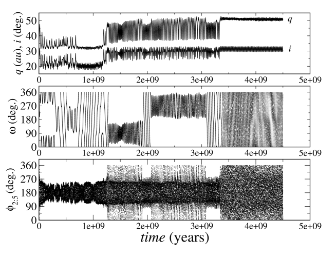
Figure 11: Time evolution of a particle captured by the 2:5 MMR with Neptune. Upper panel shows the evolution of the perihelion distance, q, and inclination, i. The middle panel shows the evolution of the argument of perihelion, $\omega$, and the bottom panel presents the resonant angle $\phi_{2:5}$. We notice several dynamical modes like the Kozai+MMR, and the hibernating mode. In the end the particle is in a non-fossilized detached orbit.

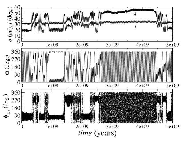
Figure 12: Time evolution of a particle captured in the 1:3 MMR with Neptune. Upper panel shows the evolution of the perihelion distance, q, and inclination, i. The middle panel shows the evolution of the argument of perihelion, $\omega$, and the bottom panel presents the resonant angle $\phi_{1:3}$. It is possible to note one of the asymmetric centers of the Kozai resonance between $800My$ and $1.4Gy$. Despite the particle remains in the hibernating mode for a long time, the resonances restart in the Kozai mode and the large perihelion variation dynamics are installed at the end of the simulation.

5 Imposing a residual migration on Neptune

We now proceed to a new set of numerical integrations with no migration. This time Jupiter, Saturn, and Uranus are at their current positions, as in the last section, while the mean semimajor axis of Neptune was decreased to $\bar{a}_{N}=29.8au$. A total of 16,000 particles were initially considered. The limits on the particles’ initial conditions and other integration parameters are equivalent to those in section 4, except that the semimajor axes of the particles are distributed around $a=54.8911\pm 1au$ and $a=61.9854\pm 1au$. This new set of integrations was done to check whether the main characteristics of the first set of integrations were maintained and to introduce the possibility of including a residual migration on Neptune for further analysis with migration. One finds that the global features are the same for the two sets of numerical simulations. Similar results are also possible in the case, as shown by Figures 11 and 12, where Neptune is placed before its actual position. One also finds that $12\%$ of the particles attain $q>40au$ regardless of whether they survive or not for the age of the solar system, but only one fourth of them reach hibernating mode. In these integrations, we identify the hibernating mode whenever $q>40au$ for $\Delta t\geq 100My$. With this condition, one can identify, in a general way, the hibernating cases inside the large data set generated by the simulations without looking one by one. Since in the hibernating mode the resonant angle circulates or librates with very large amplitude, these particles become potential candidates to fossilization while Neptune migrates.

With these simulations we want to understand the behavior of the particles when Neptune is still migrating to its current position. To accomplish this task we artificially added a force that depends on the velocity components into Neptune’s equations of motion in order to linearly increase its semimajor axis. Our idea was to study the final phase of a planetary migration. We considered that Neptune’s migration speed comes from the Nice model integration described in Section 2. We also note that for a smooth migration, roughly the same migration speeds are obtained. This result argues for the robustness of the mechanism presented here. We only consider Neptune’s migration since the farther planet migrates much faster than the others, and dynamical processes experienced by TNOs (like mean motion resonances) are almost solely related to Neptune.

The first experiment consisted of choosing two different points in the orbital evolution of a particle. For one of these points, the particle is experiencing the Kozai dynamics with strong variations in the eccentricity and the inclination, and the particle is in the hibernating mode for the other point. In this experiment we only considered that particle and the planets at those two chosen times. For either point (particle and time), new integrations were started as many times as the chosen migration speeds for Neptune in the interval $[0.1;5.0]au/Gy$, with steps of $0.01au/Gy$. Therefore, the resonant semimajor axis also migrates. The simulations were stopped whenever Neptune reaches its current average semimajor axis of $30.11au$.

By this experiment it is possible to check the particle’s ability to escape from each dynamical mode and get fossilized in a smaller semimajor axis than the resonant ones. It is also possible to verify whether such escapes are related to the migration speed of Neptune. Figures 13 and 14 show the results of Neptune’s migration rates as a function of the averaged semimajor axis over the final $5\%$ of each integration for particles that were initially in the regions of the 2:5 MMR and 1:3 MMR, respectively. They also show the approximate values of the resonant semimajor axis at the beginning and end of Neptune’s residual migration . It is noted that in almost $100\%$ of the cases initially in Kozai dynamics, the particles tend to follow Neptune’s migration, and continue captured in the MMRs.

There are a few cases where the particle started in the Kozai dynamics and escaped the MMR (Figure 14). Analyzing the data from these simulations, one notices that, before the particle escaped the resonance, it switched to the hibernating mode. As for the case where the particles begin in the hibernating mode (filled circles) one has the opposite situation, where most particles tend to escape the MMR easily, being fossilized without migrating. In the simulations where the particle was initially in the hibernating mode and followed Neptune’s migration, we also observed that it switched the dynamic mode (from hibernating to Kozai) before starting the migration. Thus, we could claim through this experiment that to become a fossilized object with low eccentricity, the particle must reach the hibernating mode while Neptune is still migrating. The escapes from resonance at a specific point in the evolution were shown to be a function almost only of whether the particle was in Kozai or hibernating mode with barely any correlation with Neptune’s migration rate in the studied range.

Figure 13: Diagram $V_{mig}$ vs. averaged semimajor axis for particles that were initially in 2:5 MMR with Neptune. The average is calculated over the past $5\%$ of each simulation. The black filled circles represent particles that started the new simulations in the hibernating mode, while the open circles represent those that started in the Kozai mode. The vertical lines are the approximate resonant semimajor axis before (at left) and after (at right) the residual migration of Neptune. It is clear that particles initially in the hibernating mode tend to escape the MMR, becoming fossilized objects, while the ones started in the Kozai mode, in the opposite way, tend to stay trapped in the MMR and follow the migration.

Figure 14: Analogous to the Figure 13 for particles that were initially close to the 1:3 MMR with Neptune.

The experiments just performed suggest that escapes from the hibernating mode is a near 100$\%$ chance event for migration speeds above 0.1$au/Gy$, thus, as Figure 2 shows, particles must escape from resonance in hibernating mode until at least 3Gy before the present date. However, it is not obvious that escapes after 1.5$Gy$ at hibernating mode are unlikely. In fact, although the migration speed is on average below 0.1$au/Gy$ during the past 3$Gy$ of integration, we notice that this speed can fluctuate between positive and negative values, being often above 0.1$au/Gy$ in absolute value. So as to check how likely escapes from resonance at hibernating mode are for Neptune migration speeds, such as those in the great integration shown in Figure 2, we performed the following experiment. Everything were the same as for the experiments that yielded Figures 13 and 14, except that the migration speed imposed on Neptune will be dictated by the migration experienced by Neptune in the great integration that yielded Figure 2. We thus computed Neptune’s migration speed through the differences in the average Neptune’s semimajor axis in successive 5$My$ time ranges. Then we applied these successive migration speeds, which was changed at every 5$My$, to Neptune coming from the static integrations. We only used the initial conditions at hibernating mode for both the 2:5 and 1:3 resonances as those used in the experiments that yielded Figures 13 and 14, in the beginning of this section. For either resonance we did 25 numerical integrations imposing Neptune’s migration speed as those from the great integration as if Neptune started at 1.6$Gy$ until 4.0$Gy$ with steps of 0.1$Gy$. All integrations extend to 4.5$Gy$. Figure 15 shows the results of this experiment, where we show Neptune’s average semimajor axis orbital evolution, and for each integration started at the time shown in the figure, we plot “E” for an escape event and “R” for a still in resonance event. We find that there are still escapes from the hibernating mode during the last 3$Gy$ of Neptune’s mild migration for a fraction between one half and one third of the cases.

Figure 15: Average evolution of Neptune’s semimajor axis with Neptune’s initial semimajor axis coming from the static integrations and experiencing migration with the same migration rates as those suffered by Neptune for the last 3Gy of the great integration shown in Figure 2. Also plotted is the result of the application of Neptune’s migration on particles started at hibernating mode:“R” stands for a particle that remained in resonance to the end of the integration and “E” for a particle that eventually escaped the resonance before the end of the integration. The time associated with either of these symbols stands for the initial time of integration with Neptune experiencing the semimajor axis evolution shown in this plot. All integrations are extended to 4.5Gy

To find the most probable values of the eccentricities for fossilized particles, after they escape the MMR, we did a complementary experiment. This time we fixed the residual migration rate of Neptune in $V_{mig}=0.5au/Gy$, a reasonable value for the final migration phase in simulations that take massive particles into account (e.g., Nice model). We chose nine particles that were initially in the 2:5 MMR region and seven other from the 1:3 MMR region. These particles show the most interesting dynamical modes, especially long periods in the hibernating mode, like those in Figures 11 and 12. Then, we took 123 points for each particle, along their original simulations and restarted them by considering a migrating Neptune. Therefore, 1107 (9x123) runs were made for 2:5 MMR particles and 861 (7x123) runs for 1:3 MMR particles. In the end, $240$ particles escaped the 2:5 MMR and $168$ particles escaped the 1:3 MMR. Figures 16 and 17 exhibit histograms for the original eccentricities distribution and for the averaged eccentricities after the MMR escapes, for particles that became fossilized for the 2:5 and 1:3 MMRs, respectively. It is noteworthy that particles that escaped the MMRs mostly have low eccentricities. It is found that the most probable values for the eccentricities are 0.12 and 0.18 ($44.9\lesssim q\lesssim 48.7au$) for the 2:5 MMR case, and 0.21 ($48.8\lesssim q\lesssim 49.3au$) for the 1:3 MMR case. These results confirm what is proposed by Gomes (2011) that orbits similar to $2004XR_{190}$ may be formed close to other MMRs.

Figure 16: Comparison between the eccentricities distribution for the evolution of the 9 original particles in the 2:5 MMR region (dotted histogram) and the averaged eccentricities for the test particles that escaped the resonance while Neptune was migrating, becoming fossilized (continuous black histogram). Peaks at $e\sim 0.12$ and $e\sim 0.18$ suggest that $2004XR_{190}$-like orbits might be formed close to 2:5 MMR with Neptune.

Figure 17: Comparison between the eccentricities distribution for the evolution of the 7 original particles in the 1:3 MMR region (dotted histogram) and the averaged eccentricities for the test particles that released the resonance while Neptune migrates, becoming fossilized (continuous black histogram). The peak at $e\sim 0.21$ suggests that $2004XR_{190}$-like orbits might be formed close to 1:3 MMR with Neptune.

The previous experiments show that it is possible to form detached objects fossilized close to the 2:5 and 1:3 MMRs. However, these experiments do not allow calculating the fraction of objects that become fossilized from the initial population, since they were chosen on purpose based on specific particles evolution in which the hibernating mode appeared. To make a more unbiased analysis that takes the total time which the particles spend in the hibernating mode into account, we performed another experiment. It consists of taking the simulations with Neptune at $29.8au$ and restart them from different times, considering that Neptune migrates with $V_{mig}=0.5au/Gy$. All bodies present at the selected times are considered. Thus it is possible to verify the formation of fossilized objects in a scenario in which several types of scattered particles are perturbed by a migrating Neptune. We consider that an object is fossilized if its average semimajor axis, after Neptune reaches its current position, is in the region $54.6<a<55.4au$ for bodies close to the 2:5 MMR or $61.8<a<62.4au$ for bodies close to the 1:3 MMR. A total of 15 simulations were performed. In all of them at least one fossilized object with $q>40au$ was formed in both regions, as shown by Table 1. However, we note that these simulations are also able to produce fossilized objects with moderate perihelion distance ($35<q<40au$). This result is qualitatively in accordance with Figures 16 and 17, which show two peaks in the distributions of detached objects, one for moderate perihelion distance and another one for high perihelion distance. Of course those figures do not show quantitative coherence since the initial conditions were chosen on purpose from orbital evolutions exhibiting the hibernating mode. Approximately 70 $\%$ of fossilized objects with moderate perihelion distance turned out to be stable for periods of billions of years on later simulations, while 100$\%$ of fossilized objects with high perihelion distance ($q>40au$) are stable. The simulations in this new experiment generated, on average, 4.22 fossilized particles with moderate perihelion distance for each fossilized object with high perihelion distance for the 2:5 MMR case, while this ratio is 2.43 to 1 for the 1:3 MMR. We continued the integration of some of the particles for an extra Gy and found out that on average 30% of the moderate perihelion distance ones did not keep stable. Thus the corrected rates not including the unstable particles should be 2.95/1 (2:5 MMR) and 1.70/1 (1:3 MMR).

Table 1: Particles fossilized with moderate and high q when Neptune achieves its current position. Left side stands for the results of the 2:5MMR runs, while the right side for the 1:3MMR. The columns represent the run ID, the number of objects fossilized with $q>40au$ ($N_{1}$), and the number of objects with $35<q<40au$ ($N_{2}$).

Run	N1	N2		Run	$N_{1}$	$N_{2}$
$\#1$	$5$	$14$		$\#1$	$3$	$5$
$\#2$	$2$	$18$		$\#2$	$4$	$8$
$\#3$	$5$	$15$		$\#3$	$3$	$8$
$\#4$	$2$	$9$		$\#4$	$5$	$11$
$\#5$	$1$	$8$		$\#5$	$5$	$7$
$\#6$	$4$	$12$		$\#6$	$4$	$10$
$\#7$	$4$	$12$		$\#7$	$4$	$10$
$\#8$	$3$	$25$		$\#8$	$2$	$11$
$\#9$	$6$	$23$		$\#9$	$3$	$10$
$\#10$	$6$	$24$		$\#10$	$3$	$12$
$\#11$	$6$	$20$		$\#11$	$1$	$8$
$\#12$	$8$	$21$		$\#12$	$3$	$10$
$\#13$	$5$	$12$		$\#13$	$6$	$3$
$\#14$	$4$	$19$		$\#14$	$4$	$8$
$\#15$	$6$	$51$		$\#15$	$8$	$20$
Tot.	$67$	$283$		Tot.	$58$	$141$

Figure 18 shows the results for the region of the 2:5 MMR for one original simulation without migration, which was restarted with Neptune’s migration from approximately 3.5 Gy, and Figure 19 presents the 1:3 MMR region for the same original simulation restarted from approximately 1Gy. Most bodies tends to remain trapped to the MMRs and follow the migration of Neptune. Nevertheless, some particles escape the resonance becoming scattered objects (below the lower horizontal line), fossilized with moderate perihelion distances (between horizontal lines and $54.6<a<55.4au$ or $61.8<a<62.4au$) or fossilized with high perihelion distance (above the upper horizontal line and $54.6<a<55.4au$ or $61.8<a<62.4au$).

The scattered objects are very moble in the semimajor axis. They are strongly perturbed by Neptune and usually end up being ejected from the solar system on hyperbolic orbits. The fossilized objects with moderate perihelion distances have less mobility in semimajor axis than the scattered ones, and most of them are stable after Neptune arrives at its current position. The fossilized objects with high perihelion distance, on the other hand, have almost no mobility in semimajor axis and are very stable, surviving by the age of the solar system after Neptune reaches its current position. Through an experiment using a more generic approach, we thus show that detached objects close to the 2:5 and 1:3 MMRs with Neptune can be generated through gravitational interactions among scattered particles and giant planets without the need of an external agent (e.g., stellar passages or planetary companion with planetary mass). We just need a scattered particle to be captured in a MMR with Neptune, to experience the Kozai resonance, and to access the hibernating mode while Neptune is still migrating to its current position.

One comment is in order with respect to the particles that remain trapped in the MMRs with Neptune in this last experiment. Since these particles amount to many more that escape, one could try to estimate the ratio of current trapped particles to escaped ones. But we do not think this experiment is suitable for that calculation. In fact, the integration with migration lasts just 600 My in view of the initial position of Neptune and the migration speed. This is justifiable since the migration is in fact exponentially damping and we are taking it as linear, and most of the migration will take place in these first 600 My. There will therefore be some 3.5 Gy left for evolution time, during which we expect that most of the resonant particles will be scattered out of the resonance.

Figure 18: Results in the region of the 2:5 MMR for one original simulation restarted from $\sim 3.5Gy$. Neptune was initially at $a_{N}=29.8$au and was made to migrate with $V_{mig}=0,5au/Gy$. The vertical lines account for the initial (at left) and final (at right) resonant semimajor axis $a_{2:5}$. All particles that were present in the original integration at that time they were considered.

Figure 19: Results in the region of the 1:3 MMR for one original simulation restarted from $\sim 1.0Gy$. Neptune was initially at $a_{N}=29.8$au and was made to migrate with $V_{mig}=0.5au/Gy$. The vertical lines account for the initial (at left) and final (at right) resonant semimajor axis $a_{1:3}$. All particles that were present in the original integration at that time were considered.

Since we considered an initial uniform distribution of inclinations between $0^{\circ}$ and $50^{\circ}$, a natural question is how the formation of fossilized detached objects depends on the initial inclination. For this we considered all integrations without migration and plot histograms of the initial inclination of all particles that experienced at least one instance of a hibernating mode. Figure 20 shows these histograms for the 2:5 and 1:3 resonances. It is interesting to compare this with Figure 5, which gives the distribution of inclinations near these resonances for the numerical integration presented in Section 2. The comparison of these two distributions will be used to better estimate the mass likely deposited near the resonances in the next section. It is interesting to note that the histogram for the 1:3 resonance is much more skewed to the left than the one for the 2:5 resonance. Although we do not attempt to explain this feature, we can confirm that it is real in the sense that a particle trapped in the 1:3 MMR with a low inclination can eventually get into Kozai resonance and experience a large amplitude couple variation of the eccentricity and inclination that brings the eccentricity to near $0.1$ and the inclination to near $30^{\circ}$. Figure 21 shows an example of such behavior.

5.1 Estimation of the mass of detached fossilized objects

Although the simulations performed here were not particularly aimed at computing the total number of detached objects that would come from a past hibernating episode, we do think that we can roughly estimate the total mass that would be deposited near the 2:5 and 1:3 resonances as fossilized objects with high perihelion distance. We consider the integrations without migration and assume that every instance of a hibernating mode creates a fossilized object with high perihelion distance, which is reasonable in view of the examples shown in Figures13 and 14. For the 2:5 resonance we find that $0.38$% of the particles show at least one instance of a hibernating mode for the first $0.85$ Gy, whereas for the 1:3 resonance this fracion is $0.55$%. Now we compare this fraction with the total mass available in the neighborhood of each resonance taken from the Nice model simulation described in Section 2. This mass at $0.75$ Gy, after which Neptune experiences an effective residual migration for $0.85$ Gy is 0.041 and 0.036 Earth masses for the 2:5 and 1:3 resonances, respectively. This yields final total masses for fossilized objects with high perihelion near those resonances as $0.07$ and $0.09$ in Pluto’s mass.

If we consider the last 3$Gy$ of planetary migration, the fractions of particles that show at least one instance of a hibernating mode is 1.8% and 2.2% for the 2:5 and 1:3 MMR, respectively. Considering the probability of escaping from the hibernating mode during the last 3 $Gy$ is around 40% as suggested by Figure 15, we estimate a total mass in the neighborhood of the 2:5 and 1:3 MMR as 0.21 and 0.26 in Pluto’s mass.

Now we must also consider that this calculation was based on a uniform distribution of the inclination from $0^{\circ}$ to $50^{\circ}$. The distribution of inclinations that yields at least one instance of a hibernating mode is shown in Figure 20. On the other hand, the expected distribution of inclinations around the 2:5 and 1:3 MMR is shown in Figure 5. To get more accurate fractions of particles that show at least one instance of a hibernating mode, we must multiply the above numbers by a factor which is the weighed sum of the fraction of particles in each bin of the distributions shown in Figure 20. The weights are given by normalizing the fractions given in Figure 5 so that the sum of these weights equals $10$, the number of bins. With this in mind we found the factors $0.88$ and $1.57$ that must multiply the estimated masses above in the neighborhood of the 2:5 and 1:3 MMR’s. The larger multiplying factor obtained for the 1:3 MMR reflects that the distribution of inclinations that yielded hibernating modes in Figure 20 is quite similar to the distribution of inclinations that particles should have near the 1:3 resonance according to Figure 5.

Figure 20: Distribution of initial inclinations of particles that yielded at least one instance of a hibernating mode episode

Figure 21: Evolution of a particle trapped in the 1:3 MMR with Neptune, experiencing the Kozai resonance and eventually the hibernating mode. The particle starts with a small inclination and shows large coupled variations of the eccentricity and inclination.

It is also helpful to consider the great simulation presented in Section 2. As noted earlier, there are one case for the 2:5 resonance and another one for the 1:3 resonance where a particle is trapped into MMR and Kozai resonance and eventually escape those resonances. Each of these particles carries roughly $0.32$ Pluto’s mass, which could be considered as another mass estimate at low eccentricities in the neighborhood of these resonances. This number is more in accordance with the mass estimate taken from the cases where we consider a longer time range during which a particle can enter and escape a hibernating mode. On the other hand, from the two examples taken from the Nice model numerical simulation, the particles that get detached near the 2:5 and 1:3 resonances are fossilized between $0.8$ and $0.9$ Gy, thus in the first $0.15$ Gy of Neptune’s residual migration. We notice, however, particles that are fossilized much later coming from resonances of higher order and farther from Neptune. One caveat in the computation of the mass through the indirect method described above is that this computation is based on the total mass (particles) at the beginning of the integration. Since in the simulations undertaken in Sects. 4 and 5 we impose artificial limits for discarding the particles the number of particles in the neighborhood of the resonances decrease much faster than reality (for instance, considering the numerical integration of Section 2) which also entails a fewer particles available to experience all the mechanism that produces the fossilized detached particles thus underestimating the total mass near those resonances. Considering all these factors, we can roughly estimate the amount of mass with low eccentricity near each of those resonances as $0.1$ to $0.3$ Pluto’s mass.

6 Conclusions

We addressed the main aspects of the dynamical formation of detached objects close to the 2:5 and 1:3 MMRs with Neptune from primordial scattered disk particles. Our simulations show that a considerable fraction of the scattered disk particles at the neighborhood of those resonances reach $q>40au$ at some point in their orbital evolution. For such an increase in perihelion, considering only the gravitational perturbation of the giant planets, it is necessary that the particle get captured in exterior mean motion resonance with Neptune and thereafter experience the Kozai resonance, which produces large variations in the inclination and perihelion. Thus it is possible that several TNOs are currently undergoing this resonance coupling, showing characteristics of detached objects. But sooner or later, the perihelion will decrease and the object may, again, be severely perturbed by Neptune.

As in Gomes (2011), we also identified the emergence of the hibernating mode on particles that suffer the coupling between MMR + KR. This mode is characterized by long periods ($t>100My$) of low eccentricity ($q>40au$) and high inclination and can be accessed when the amplitude of oscillation of the resonant angle, $\phi$, becomes very high ($>100^{\circ}$). Through the semi-analytical approach, for the cases of 2:5 and 1:3, we have shown the topological changes in the energy level curves associated with the hibernating mode. However, if there is no dissipative mechanism, the particle can return to experience the large amplitude anti-phase variation of the eccentricity and inclination characteristic of MMR+KR.

Through experiments considering the residual migration of Neptune, we show that the hibernating mode is a preponderant factor in the formation of fossilized objects with high perihelion, outside the resonant semimajor axis and without the possibility of suffering the Kozai mechanism again. Besides these high perihelion fossilized particles we also found objects with moderate perihelion distance ($35<q<40au$) through numerical experiments. They are not associated with the hibernating mode. We estimate that the ratio of the number of moderate-to-high perihelion objects fossilized near the 2:5 and 1:3 resonances are 2.95:1 and 1.70:1, respectively. It is important to note however that these ratios must not represent real observations since observational bias makes it easier to observe objects with smaller perihelia. We also roughly estimated the amount of mass with low eccentricity near either of those resonances as $0.1$ to $0.3$ Pluto’s mass.

As shown here for the resonances 2:5 and 1:3, and 3:8 by Gomes (2011), the same mechanism could act in other MMRs in the trans-Neptunian region, forming other groups of detached objects, mostly for MMRs with $a<100au$. In principle, since there are some MMR with Neptune in the classical Kuiper belt (e.g., 4:7, 3:5, 5:8), it is possible that the same process could also be effective near those resonances and contribute to the formation of part of hot classical Kuiper belt objects (HCKBOs). We can anticipate that in preliminary tests, the hibernating mode showed up for some of the resonances in the classical belt. However, determining the efficiency of the process, as well as its relative contribution to the HCKBOs group, deserves further investigation that is going to be the subject of future works.