1 Introduction
Interface problems for partial differential equations (PDEs) are initial boundary value problems for which the solution of an equation in one domain prescribes boundary conditions for the equations in adjacent domains. In applications, precise interface conditions follow from conservations laws. Few interface problems allow for an explicit closed-form solution using classical solution methods. Using the Fokas method [7 , 8 , 9 ] such solutions may be constructed for both dissipative and dispersive linear interface problems.
In two recent papers [2 , 6 ] this was done for the classical problem of the heat equation. In [6 ] the main application considered is that of heat flow in composite walls or rods while in [2 ] the heat equation is viewed as a simplified reaction-diffusion equation describing the spreading of tumors in the brain. Problems in both finite and infinite domains were investigated in [6 ] and the method was compared with classical solution approaches if such exist [4 , 10 ] . The same is done here for the linear Schrödinger (LS) equation with an interface. We restrict to the case of a continuous wave function with a jump in the derivative across the interface. Although the problem and the method considered here are similar to the one presented in [2 ] and [6 ] , the dispersive nature of the problem makes it more difficult to solve both classically and using the method of Fokas.
The linear Schrödinger equation is arguably the simplest dispersive equation, having the dispersion relation ω ( k ) = k 2 𝜔 𝑘 superscript 𝑘 2 \omega(k)=k^{2} [14 ] , and as the linearization of various nonlinear equations, most notably the nonlinear Schrödinger (NLS) equations i q t ( x , t ) = − q x x ( x , t ) ± | q ( x , t ) | 2 q ( x , t ) 𝑖 subscript 𝑞 𝑡 𝑥 𝑡 plus-or-minus subscript 𝑞 𝑥 𝑥 𝑥 𝑡 superscript 𝑞 𝑥 𝑡 2 𝑞 𝑥 𝑡 iq_{t}(x,t)=-q_{xx}(x,t)\pm|q(x,t)|^{2}q(x,t) [18 ] , plasma physics [17 ] , nonlinear fiber optics [11 , 12 ] , magneto-static spin waves [19 ] , and many other settings.
The LS equation describes the behavior of solutions of the NLS equation in the small amplitude limit and understanding it dynamics is fundamental in understanding the dynamics of the more complicated nonlinear problem.
Recently Cascaval and Hunter [5 ] have considered the time-dependent LS on simple networks. Their solution formulas are not explicit, as they contain implicit integral equations for the interface conditions. Their analysis is easily extended to more than two domains and also considers the nonlinear Schrödinger (NLS) equation. Some work has been done using the Fokas Method for moving boundary value problems in the case when the movement of the boundary is prescribed [FokasPelloni5 ] . In some cases, the solution of such problems requires the use of the “d-bar method” which reduces the problem to a linear integral equation.
The LS equation in two semi-infinite domains with an interface is considered in Section 2 3 [13 , 15 ] . Throughout, our emphasis is on non-steady state solutions. The solutions presented here using the Fokas Method are explicit and depend only on known quantities. Although we present solution formulas only for the case of two domains (both finite or both infinite) it is straightforward to generalize this method to n 𝑛 n [6 ] (three domains, both finite and infinite) and in [2 ] (n 𝑛 n
2 Two semi-infinite domains
We wish to find q L ( x , t ) superscript 𝑞 𝐿 𝑥 𝑡 q^{L}(x,t) q R ( x , t ) superscript 𝑞 𝑅 𝑥 𝑡 q^{R}(x,t)
i q t L ( x , t ) = 𝑖 subscript superscript 𝑞 𝐿 𝑡 𝑥 𝑡 absent \displaystyle iq^{L}_{t}(x,t)= σ L q x x L ( x , t ) , subscript 𝜎 𝐿 subscript superscript 𝑞 𝐿 𝑥 𝑥 𝑥 𝑡 \displaystyle\sigma_{L}q^{L}_{xx}(x,t),~{}~{}~{} − ∞ < absent \displaystyle-\infty< x < 0 , 𝑥 0 \displaystyle x<0,~{} t > 0 , 𝑡 0 \displaystyle t>0, (1)
i q t R ( x , t ) = 𝑖 subscript superscript 𝑞 𝑅 𝑡 𝑥 𝑡 absent \displaystyle iq^{R}_{t}(x,t)= σ R q x x R ( x , t ) , subscript 𝜎 𝑅 subscript superscript 𝑞 𝑅 𝑥 𝑥 𝑥 𝑡 \displaystyle\sigma_{R}q^{R}_{xx}(x,t),~{}~{}~{} 0 < 0 absent \displaystyle 0< x < ∞ , 𝑥 \displaystyle x<\infty,~{} t > 0 , 𝑡 0 \displaystyle t>0,
subject to the asymptotic conditions
lim x → − ∞ q L ( x , t ) = subscript → 𝑥 superscript 𝑞 𝐿 𝑥 𝑡 absent \displaystyle\lim_{x\to-\infty}q^{L}(x,t)= γ L , subscript 𝛾 𝐿 \displaystyle\gamma_{L}, (2)
lim x → ∞ q R ( x , t ) = subscript → 𝑥 superscript 𝑞 𝑅 𝑥 𝑡 absent \displaystyle\lim_{x\to\infty}q^{R}(x,t)= γ R , subscript 𝛾 𝑅 \displaystyle\gamma_{R},
the initial conditions
q L ( x , 0 ) = superscript 𝑞 𝐿 𝑥 0 absent \displaystyle q^{L}(x,0)= q 0 L ( x ) , subscript superscript 𝑞 𝐿 0 𝑥 \displaystyle q^{L}_{0}(x),~{}~{}~{} − ∞ \displaystyle-\infty < x < 0 , absent 𝑥 0 \displaystyle<x<0, (3)
q R ( x , 0 ) = superscript 𝑞 𝑅 𝑥 0 absent \displaystyle q^{R}(x,0)= q 0 R ( x ) , subscript superscript 𝑞 𝑅 0 𝑥 \displaystyle q^{R}_{0}(x),~{}~{}~{} 0 0 \displaystyle 0 < x < ∞ , absent 𝑥 \displaystyle<x<\infty,
and the interface conditions
q L ( 0 , t ) = superscript 𝑞 𝐿 0 𝑡 absent \displaystyle q^{L}(0,t)= q R ( 0 , t ) , superscript 𝑞 𝑅 0 𝑡 \displaystyle q^{R}(0,t),~{}~{}~{} t > 0 , 𝑡 0 \displaystyle t>0, (4)
β L q x L ( 0 , t ) = subscript 𝛽 𝐿 subscript superscript 𝑞 𝐿 𝑥 0 𝑡 absent \displaystyle\beta_{L}q^{L}_{x}(0,t)= β R q x R ( 0 , t ) , subscript 𝛽 𝑅 subscript superscript 𝑞 𝑅 𝑥 0 𝑡 \displaystyle\beta_{R}q^{R}_{x}(0,t),~{}~{}~{} t > 0 , 𝑡 0 \displaystyle t>0,
where γ L , γ R , σ L , σ R , β L subscript 𝛾 𝐿 subscript 𝛾 𝑅 subscript 𝜎 𝐿 subscript 𝜎 𝑅 subscript 𝛽 𝐿
\gamma_{L},\gamma_{R},\sigma_{L},\sigma_{R},\beta_{L} β R subscript 𝛽 𝑅 \beta_{R} t 𝑡 t L 𝐿 L R 𝑅 R σ L subscript 𝜎 𝐿 \sigma_{L} σ R subscript 𝜎 𝑅 \sigma_{R}
First, we shift the problem so that the asymptotic conditions are identically zero. We define v L ( x , t ) = q L ( x , t ) − γ L superscript 𝑣 𝐿 𝑥 𝑡 superscript 𝑞 𝐿 𝑥 𝑡 subscript 𝛾 𝐿 v^{L}(x,t)=q^{L}(x,t)-\gamma_{L} v R ( x , t ) = q R ( x , t ) − γ R superscript 𝑣 𝑅 𝑥 𝑡 superscript 𝑞 𝑅 𝑥 𝑡 subscript 𝛾 𝑅 v^{R}(x,t)=q^{R}(x,t)-\gamma_{R}
i v t L ( x , t ) = 𝑖 subscript superscript 𝑣 𝐿 𝑡 𝑥 𝑡 absent \displaystyle iv^{L}_{t}(x,t)= σ L v x x L ( x , t ) , subscript 𝜎 𝐿 subscript superscript 𝑣 𝐿 𝑥 𝑥 𝑥 𝑡 \displaystyle\sigma_{L}v^{L}_{xx}(x,t), − ∞ < absent \displaystyle-\infty< x < 0 , 𝑥 0 \displaystyle x<0, t ≥ 0 , 𝑡 0 \displaystyle t\geq 0, (5a)
i v t R ( x , t ) = 𝑖 subscript superscript 𝑣 𝑅 𝑡 𝑥 𝑡 absent \displaystyle iv^{R}_{t}(x,t)= σ R v x x R ( x , t ) , subscript 𝜎 𝑅 subscript superscript 𝑣 𝑅 𝑥 𝑥 𝑥 𝑡 \displaystyle\sigma_{R}v^{R}_{xx}(x,t), 0 < 0 absent \displaystyle 0< x < ∞ , 𝑥 \displaystyle x<\infty, t ≥ 0 , 𝑡 0 \displaystyle t\geq 0, (5b)
lim x → − ∞ v L ( x , t ) = subscript → 𝑥 superscript 𝑣 𝐿 𝑥 𝑡 absent \displaystyle\lim_{x\to-\infty}v^{L}(x,t)= 0 , 0 \displaystyle 0, t ≥ 0 , 𝑡 0 \displaystyle t\geq 0, (5c)
lim x → ∞ v R ( x , t ) = subscript → 𝑥 superscript 𝑣 𝑅 𝑥 𝑡 absent \displaystyle\lim_{x\to\infty}v^{R}(x,t)= 0 , 0 \displaystyle 0, t ≥ 0 , 𝑡 0 \displaystyle t\geq 0, (5d)
v L ( x , 0 ) = superscript 𝑣 𝐿 𝑥 0 absent \displaystyle v^{L}(x,0)= v 0 L ( x ) , subscript superscript 𝑣 𝐿 0 𝑥 \displaystyle v^{L}_{0}(x), − ∞ < absent \displaystyle-\infty< x < 0 , 𝑥 0 \displaystyle x<0, (5e)
v R ( x , 0 ) = superscript 𝑣 𝑅 𝑥 0 absent \displaystyle v^{R}(x,0)= v 0 R ( x ) , subscript superscript 𝑣 𝑅 0 𝑥 \displaystyle v^{R}_{0}(x), 0 < 0 absent \displaystyle 0< x < ∞ , 𝑥 \displaystyle x<\infty, (5f)
v L ( 0 , t ) + γ L = superscript 𝑣 𝐿 0 𝑡 superscript 𝛾 𝐿 absent \displaystyle v^{L}(0,t)+\gamma^{L}= v R ( 0 , t ) + γ R , superscript 𝑣 𝑅 0 𝑡 superscript 𝛾 𝑅 \displaystyle v^{R}(0,t)+\gamma^{R}, t ≥ 0 , 𝑡 0 \displaystyle t\geq 0, (5g)
β L v x L ( 0 , t ) = subscript 𝛽 𝐿 subscript superscript 𝑣 𝐿 𝑥 0 𝑡 absent \displaystyle\beta_{L}v^{L}_{x}(0,t)= β R v x R ( 0 , t ) , subscript 𝛽 𝑅 subscript superscript 𝑣 𝑅 𝑥 0 𝑡 \displaystyle\beta_{R}v^{R}_{x}(0,t), t ≥ 0 . 𝑡 0 \displaystyle t\geq 0. (5h)
We follow the standard steps in the application of the Fokas Method [7 , 8 , 9 ] , beginning with the so-called “local relations” [7 ]
( e − i k x + λ L t v L ( x , t ) ) t = subscript superscript 𝑒 𝑖 𝑘 𝑥 subscript 𝜆 𝐿 𝑡 superscript 𝑣 𝐿 𝑥 𝑡 𝑡 absent \displaystyle\left(e^{-ikx+{\color[rgb]{0,0,0}\lambda_{L}}t}v^{L}(x,t)\right)_{t}= ( σ L e − i k x + λ L t ( k v L ( x , t ) − i v x L ( x , t ) ) ) x , subscript subscript 𝜎 𝐿 superscript 𝑒 𝑖 𝑘 𝑥 subscript 𝜆 𝐿 𝑡 𝑘 superscript 𝑣 𝐿 𝑥 𝑡 𝑖 subscript superscript 𝑣 𝐿 𝑥 𝑥 𝑡 𝑥 \displaystyle\left(\sigma_{L}e^{-ikx+{\color[rgb]{0,0,0}\lambda_{L}}t}(kv^{L}(x,t)-iv^{L}_{x}(x,t))\right)_{x},~{}~{}~{} − ∞ < absent \displaystyle-\infty< x < 0 , 𝑥 0 \displaystyle x<0, (6a)
( e − i k x + λ R t v R ( x , t ) ) t = subscript superscript 𝑒 𝑖 𝑘 𝑥 subscript 𝜆 𝑅 𝑡 superscript 𝑣 𝑅 𝑥 𝑡 𝑡 absent \displaystyle\left(e^{-ikx+{\color[rgb]{0,0,0}\lambda_{R}}t}v^{R}(x,t)\right)_{t}= ( σ R e − i k x + λ R t ( k v R ( x , t ) − i v x R ( x , t ) ) ) x , subscript subscript 𝜎 𝑅 superscript 𝑒 𝑖 𝑘 𝑥 subscript 𝜆 𝑅 𝑡 𝑘 superscript 𝑣 𝑅 𝑥 𝑡 𝑖 subscript superscript 𝑣 𝑅 𝑥 𝑥 𝑡 𝑥 \displaystyle\left(\sigma_{R}e^{-ikx+{\color[rgb]{0,0,0}\lambda_{R}}t}(kv^{R}(x,t)-iv^{R}_{x}(x,t))\right)_{x},~{}~{}~{} 0 < 0 absent \displaystyle 0< x < ∞ . 𝑥 \displaystyle x<\infty. (6b)
Figure 1: Domains for the application of Green’s Theorem for v L ( x , t ) superscript 𝑣 𝐿 𝑥 𝑡 v^{L}(x,t) v R ( x , t ) superscript 𝑣 𝑅 𝑥 𝑡 v^{R}(x,t)
These are parameter relations obtained by rewriting (5a 5b λ L = − i σ L k 2 subscript 𝜆 𝐿 𝑖 subscript 𝜎 𝐿 superscript 𝑘 2 {\color[rgb]{0,0,0}\lambda_{L}}=-i\sigma_{L}k^{2} λ R = − i σ R k 2 subscript 𝜆 𝑅 𝑖 subscript 𝜎 𝑅 superscript 𝑘 2 {\color[rgb]{0,0,0}\lambda_{R}}=-i\sigma_{R}k^{2} The functions λ L ( k ) subscript 𝜆 𝐿 𝑘 \lambda_{L}(k) λ R ( k ) subscript 𝜆 𝑅 𝑘 \lambda_{R}(k) λ L = − i ω L subscript 𝜆 𝐿 𝑖 subscript 𝜔 𝐿 \lambda_{L}=-i\omega_{L} λ R = − i ω R subscript 𝜆 𝑅 𝑖 subscript 𝜔 𝑅 \lambda_{R}=-i\omega_{R} Applying Green’s Theorem [1 ] in the strip ( − ∞ , 0 ) × ( 0 , t ) 0 0 𝑡 (-\infty,0)\times(0,t) 1
0 = 0 absent \displaystyle 0= ∫ − ∞ 0 e − i k x v 0 L ( x ) d x − ∫ − ∞ 0 e − i k x + λ L t v L ( x , t ) d x + ∫ 0 t σ L e λ L s ( k v L ( 0 , s ) − i v x L ( 0 , s ) ) d s , superscript subscript 0 superscript 𝑒 𝑖 𝑘 𝑥 superscript subscript 𝑣 0 𝐿 𝑥 differential-d 𝑥 superscript subscript 0 superscript 𝑒 𝑖 𝑘 𝑥 subscript 𝜆 𝐿 𝑡 superscript 𝑣 𝐿 𝑥 𝑡 differential-d 𝑥 superscript subscript 0 𝑡 subscript 𝜎 𝐿 superscript 𝑒 subscript 𝜆 𝐿 𝑠 𝑘 superscript 𝑣 𝐿 0 𝑠 𝑖 subscript superscript 𝑣 𝐿 𝑥 0 𝑠 differential-d 𝑠 \displaystyle\int_{-\infty}^{0}e^{-ikx}v_{0}^{L}(x)\,\mathrm{d}x-\int_{-\infty}^{0}e^{-ikx+{\color[rgb]{0,0,0}\lambda_{L}}t}v^{L}(x,t)\,\mathrm{d}x+\int_{0}^{t}\sigma_{L}e^{{\color[rgb]{0,0,0}\lambda_{L}}s}\left(kv^{L}(0,s)-iv^{L}_{x}(0,s)\right)\,\mathrm{d}s, (7a)
0 = 0 absent \displaystyle 0= ∫ 0 ∞ e − i k x v 0 R ( x ) d x − ∫ 0 ∞ e − i k x + λ R t v R ( x , t ) d x − ∫ 0 t σ R e λ R s ( k v R ( 0 , s ) − i v x R ( 0 , s ) ) d s . superscript subscript 0 superscript 𝑒 𝑖 𝑘 𝑥 superscript subscript 𝑣 0 𝑅 𝑥 differential-d 𝑥 superscript subscript 0 superscript 𝑒 𝑖 𝑘 𝑥 subscript 𝜆 𝑅 𝑡 superscript 𝑣 𝑅 𝑥 𝑡 differential-d 𝑥 superscript subscript 0 𝑡 subscript 𝜎 𝑅 superscript 𝑒 subscript 𝜆 𝑅 𝑠 𝑘 superscript 𝑣 𝑅 0 𝑠 𝑖 subscript superscript 𝑣 𝑅 𝑥 0 𝑠 differential-d 𝑠 \displaystyle\int_{0}^{\infty}e^{-ikx}v_{0}^{R}(x)\,\mathrm{d}x-\int_{0}^{\infty}e^{-ikx+{\color[rgb]{0,0,0}\lambda_{R}}t}v^{R}(x,t)\,\mathrm{d}x-\int_{0}^{t}\sigma_{R}e^{{\color[rgb]{0,0,0}\lambda_{R}}s}\left(kv^{R}(0,s)-iv^{R}_{x}(0,s)\right)\,\mathrm{d}s. (7b)
Let ℂ + = { z ∈ ℂ : Im ( z ) ≥ 0 } superscript ℂ conditional-set 𝑧 ℂ Im 𝑧 0 \mathbb{C}^{+}=\{z\in\mathbb{C}:\operatorname{Im}(z)\geq 0\} ℂ − = { z ∈ ℂ : Im ( z ) ≤ 0 } superscript ℂ conditional-set 𝑧 ℂ Im 𝑧 0 \mathbb{C}^{-}=\{z\in\mathbb{C}:\operatorname{Im}(z)\leq 0\} 7 k ∈ ℂ + 𝑘 superscript ℂ k\in\mathbb{C}^{+} 7a k ∈ ℂ − 𝑘 superscript ℂ k\in\mathbb{C}^{-} 7b k ∈ ℂ 𝑘 ℂ k\in\mathbb{C}
g 0 ( ω , t ) = subscript 𝑔 0 𝜔 𝑡 absent \displaystyle g_{0}({\omega},t)= ∫ 0 t e ω s v L ( 0 , s ) d s = ∫ 0 t e ω s ( v R ( 0 , s ) + γ R − γ L ) d s superscript subscript 0 𝑡 superscript 𝑒 𝜔 𝑠 superscript 𝑣 𝐿 0 𝑠 differential-d 𝑠 superscript subscript 0 𝑡 superscript 𝑒 𝜔 𝑠 superscript 𝑣 𝑅 0 𝑠 superscript 𝛾 𝑅 superscript 𝛾 𝐿 differential-d 𝑠 \displaystyle\int_{0}^{t}e^{\omega s}v^{L}(0,s)\,\mathrm{d}s=\int_{0}^{t}e^{\omega s}(v^{R}(0,s)+\gamma^{R}-\gamma^{L})\,\mathrm{d}s
= \displaystyle= ( γ R − γ L ) ( e ω t − 1 ) ω + ∫ 0 t e ω s v R ( 0 , s ) d s , superscript 𝛾 𝑅 superscript 𝛾 𝐿 superscript 𝑒 𝜔 𝑡 1 𝜔 superscript subscript 0 𝑡 superscript 𝑒 𝜔 𝑠 superscript 𝑣 𝑅 0 𝑠 differential-d 𝑠 \displaystyle\frac{(\gamma^{R}-\gamma^{L})(e^{\omega t}-1)}{\omega}+\int_{0}^{t}e^{\omega s}v^{R}(0,s)\,\mathrm{d}s,
g 1 ( ω , t ) = subscript 𝑔 1 𝜔 𝑡 absent \displaystyle g_{1}({\omega},t)= ∫ 0 t e ω s v x L ( 0 , s ) d s = β R β L ∫ 0 t e ω s v x R ( 0 , s ) d s , superscript subscript 0 𝑡 superscript 𝑒 𝜔 𝑠 subscript superscript 𝑣 𝐿 𝑥 0 𝑠 differential-d 𝑠 subscript 𝛽 𝑅 subscript 𝛽 𝐿 superscript subscript 0 𝑡 superscript 𝑒 𝜔 𝑠 subscript superscript 𝑣 𝑅 𝑥 0 𝑠 differential-d 𝑠 \displaystyle\int_{0}^{t}e^{{\omega}s}v^{L}_{x}(0,s)\,\mathrm{d}s=\frac{\beta_{R}}{\beta_{L}}\int_{0}^{t}e^{{\omega}s}v^{R}_{x}(0,s)\,\mathrm{d}s,
v ^ L ( k , t ) = superscript ^ 𝑣 𝐿 𝑘 𝑡 absent \displaystyle\hat{v}^{L}(k,t)= ∫ − ∞ 0 e − i k x v L ( x , t ) d x , superscript subscript 0 superscript 𝑒 𝑖 𝑘 𝑥 superscript 𝑣 𝐿 𝑥 𝑡 differential-d 𝑥 \displaystyle\int_{-\infty}^{0}e^{-ikx}v^{L}(x,t)\,\mathrm{d}x, v ^ 0 L ( k ) = subscript superscript ^ 𝑣 𝐿 0 𝑘 absent \displaystyle\hat{v}^{L}_{0}(k)= ∫ − ∞ 0 e − i k x v 0 L ( x ) d x , superscript subscript 0 superscript 𝑒 𝑖 𝑘 𝑥 subscript superscript 𝑣 𝐿 0 𝑥 differential-d 𝑥 \displaystyle\int_{-\infty}^{0}e^{-ikx}v^{L}_{0}(x)\,\mathrm{d}x,
v ^ R ( k , t ) = superscript ^ 𝑣 𝑅 𝑘 𝑡 absent \displaystyle\hat{v}^{R}(k,t)= ∫ 0 ∞ e − i k x v R ( x , t ) d x , superscript subscript 0 superscript 𝑒 𝑖 𝑘 𝑥 superscript 𝑣 𝑅 𝑥 𝑡 differential-d 𝑥 \displaystyle\int_{0}^{\infty}e^{-ikx}v^{R}(x,t)\,\mathrm{d}x, v ^ 0 R ( k ) = subscript superscript ^ 𝑣 𝑅 0 𝑘 absent \displaystyle\hat{v}^{R}_{0}(k)= ∫ 0 ∞ e − i k x v 0 R ( x ) d x . superscript subscript 0 superscript 𝑒 𝑖 𝑘 𝑥 subscript superscript 𝑣 𝑅 0 𝑥 differential-d 𝑥 \displaystyle\int_{0}^{\infty}e^{-ikx}v^{R}_{0}(x)\,\mathrm{d}x.
Using these definitions, the global relations (7
0 = 0 absent \displaystyle 0= v ^ 0 L ( k ) − e λ L t v ^ L ( k , t ) + k σ L g 0 ( λ L , t ) − i σ L g 1 ( λ L , t ) , superscript subscript ^ 𝑣 0 𝐿 𝑘 superscript 𝑒 subscript 𝜆 𝐿 𝑡 superscript ^ 𝑣 𝐿 𝑘 𝑡 𝑘 subscript 𝜎 𝐿 subscript 𝑔 0 subscript 𝜆 𝐿 𝑡 𝑖 subscript 𝜎 𝐿 subscript 𝑔 1 subscript 𝜆 𝐿 𝑡 \displaystyle\hat{v}_{0}^{L}(k)-e^{{\color[rgb]{0,0,0}\lambda_{L}}t}\hat{v}^{L}(k,t)+k\sigma_{L}g_{0}({\color[rgb]{0,0,0}\lambda_{L}},t)-i\sigma_{L}g_{1}({\color[rgb]{0,0,0}\lambda_{L}},t), (8a)
0 = 0 absent \displaystyle 0= v ^ 0 R ( k ) − e λ R t v ^ R ( k , t ) − k σ R g 0 ( λ R , t ) + i ( γ R − γ L ) k ( e λ R t − 1 ) + i σ R β L β R g 1 ( λ R , t ) , superscript subscript ^ 𝑣 0 𝑅 𝑘 superscript 𝑒 subscript 𝜆 𝑅 𝑡 superscript ^ 𝑣 𝑅 𝑘 𝑡 𝑘 subscript 𝜎 𝑅 subscript 𝑔 0 subscript 𝜆 𝑅 𝑡 𝑖 subscript 𝛾 𝑅 subscript 𝛾 𝐿 𝑘 superscript 𝑒 subscript 𝜆 𝑅 𝑡 1 𝑖 subscript 𝜎 𝑅 subscript 𝛽 𝐿 subscript 𝛽 𝑅 subscript 𝑔 1 subscript 𝜆 𝑅 𝑡 \displaystyle\hat{v}_{0}^{R}(k)-e^{{\color[rgb]{0,0,0}\lambda_{R}}t}\hat{v}^{R}(k,t)-k\sigma_{R}g_{0}({\color[rgb]{0,0,0}\lambda_{R}},t)+\frac{i(\gamma_{R}-\gamma_{L})}{k}(e^{{\color[rgb]{0,0,0}\lambda_{R}}t}-1)+\frac{i\sigma_{R}\beta_{L}}{\beta_{R}}g_{1}({\color[rgb]{0,0,0}\lambda_{R}},t), (8b)
where k ∈ ℂ + 𝑘 superscript ℂ k\in\mathbb{C}^{+} 8a k ∈ ℂ − 𝑘 superscript ℂ k\in\mathbb{C}^{-} 8b the functions λ R subscript 𝜆 𝑅 \lambda_{R} λ L subscript 𝜆 𝐿 \lambda_{L} are invariant under k → − k → 𝑘 𝑘 k\to-k 8 − k 𝑘 -k
0 = 0 absent \displaystyle 0= v ^ 0 L ( − k ) − e λ L t v ^ L ( − k , t ) − k σ L g 0 ( λ L , t ) − i σ L g 1 ( λ L , t ) , superscript subscript ^ 𝑣 0 𝐿 𝑘 superscript 𝑒 subscript 𝜆 𝐿 𝑡 superscript ^ 𝑣 𝐿 𝑘 𝑡 𝑘 subscript 𝜎 𝐿 subscript 𝑔 0 subscript 𝜆 𝐿 𝑡 𝑖 subscript 𝜎 𝐿 subscript 𝑔 1 subscript 𝜆 𝐿 𝑡 \displaystyle\hat{v}_{0}^{L}(-k)-e^{{\color[rgb]{0,0,0}\lambda_{L}}t}\hat{v}^{L}(-k,t)-k\sigma_{L}g_{0}({\color[rgb]{0,0,0}\lambda_{L}},t)-i\sigma_{L}g_{1}({\color[rgb]{0,0,0}\lambda_{L}},t), (9a)
0 = 0 absent \displaystyle 0= v ^ 0 R ( − k ) − e λ R t v ^ R ( − k , t ) + k σ R g 0 ( λ R , t ) − i ( γ R − γ L ) k ( e λ R t − 1 ) + i σ R β L β R g 1 ( λ R , t ) , superscript subscript ^ 𝑣 0 𝑅 𝑘 superscript 𝑒 subscript 𝜆 𝑅 𝑡 superscript ^ 𝑣 𝑅 𝑘 𝑡 𝑘 subscript 𝜎 𝑅 subscript 𝑔 0 subscript 𝜆 𝑅 𝑡 𝑖 subscript 𝛾 𝑅 subscript 𝛾 𝐿 𝑘 superscript 𝑒 subscript 𝜆 𝑅 𝑡 1 𝑖 subscript 𝜎 𝑅 subscript 𝛽 𝐿 subscript 𝛽 𝑅 subscript 𝑔 1 subscript 𝜆 𝑅 𝑡 \displaystyle\hat{v}_{0}^{R}(-k)-e^{{\color[rgb]{0,0,0}\lambda_{R}}t}\hat{v}^{R}(-k,t)+k\sigma_{R}g_{0}({\color[rgb]{0,0,0}\lambda_{R}},t)-\frac{i(\gamma_{R}-\gamma_{L})}{k}(e^{{\color[rgb]{0,0,0}\lambda_{R}}t}-1)+\frac{i\sigma_{R}\beta_{L}}{\beta_{R}}g_{1}({\color[rgb]{0,0,0}\lambda_{R}},t), (9b)
where k ∈ ℂ − 𝑘 superscript ℂ k\in\mathbb{C}^{-} 9a k ∈ ℂ + 𝑘 superscript ℂ k\in\mathbb{C}^{+} 9b
Inverting the Fourier transform in (8a
v L ( x , t ) = 1 2 π ∫ − ∞ ∞ e i k x − λ L t v ^ 0 L ( k ) d k + 1 2 π ∫ − ∞ ∞ e i k x − λ L t σ L ( k g 0 ( λ L , t ) − i g 1 ( λ L , t ) ) d k , superscript 𝑣 𝐿 𝑥 𝑡 1 2 𝜋 superscript subscript superscript 𝑒 𝑖 𝑘 𝑥 subscript 𝜆 𝐿 𝑡 superscript subscript ^ 𝑣 0 𝐿 𝑘 differential-d 𝑘 1 2 𝜋 superscript subscript superscript 𝑒 𝑖 𝑘 𝑥 subscript 𝜆 𝐿 𝑡 subscript 𝜎 𝐿 𝑘 subscript 𝑔 0 subscript 𝜆 𝐿 𝑡 𝑖 subscript 𝑔 1 subscript 𝜆 𝐿 𝑡 differential-d 𝑘 v^{L}(x,t)=\frac{1}{2\pi}\int_{-\infty}^{\infty}e^{ikx-{\color[rgb]{0,0,0}\lambda_{L}}t}\hat{v}_{0}^{L}(k)\,\mathrm{d}k+\frac{1}{2\pi}\int_{-\infty}^{\infty}e^{ikx-{\color[rgb]{0,0,0}\lambda_{L}}t}\sigma_{L}(kg_{0}({\color[rgb]{0,0,0}\lambda_{L}},t)-ig_{1}({\color[rgb]{0,0,0}\lambda_{L}},t))\,\mathrm{d}k,
for − ∞ < x < 0 𝑥 0 -\infty<x<0 t > 0 𝑡 0 t>0 D = { k ∈ ℂ : Re ( − i k 2 ) < 0 } = D + ∪ D − 𝐷 conditional-set 𝑘 ℂ Re 𝑖 superscript 𝑘 2 0 superscript 𝐷 superscript 𝐷 D=\{k\in\mathbb{C}:\operatorname{Re}({-ik^{2}})<0\}=D^{+}\cup D^{-} D 𝐷 D 2 k → ∞ → 𝑘 k\to\infty k ∈ ℂ − ∖ D − 𝑘 superscript ℂ superscript 𝐷 k\in\mathbb{C}^{-}\setminus D^{-} [1 ] we can replace the contour of integration of the second integral by − ∫ ∂ D − subscript superscript 𝐷 -\int_{\partial D^{-}}
v L ( x , t ) = 1 2 π ∫ − ∞ ∞ e i k x − λ L t v ^ 0 L ( k ) d k − 1 2 π ∫ ∂ D − e i k x − λ L t σ L ( k g 0 ( λ L , t ) − i g 1 ( λ L , t ) ) d k . superscript 𝑣 𝐿 𝑥 𝑡 1 2 𝜋 superscript subscript superscript 𝑒 𝑖 𝑘 𝑥 subscript 𝜆 𝐿 𝑡 superscript subscript ^ 𝑣 0 𝐿 𝑘 differential-d 𝑘 1 2 𝜋 subscript superscript 𝐷 superscript 𝑒 𝑖 𝑘 𝑥 subscript 𝜆 𝐿 𝑡 subscript 𝜎 𝐿 𝑘 subscript 𝑔 0 subscript 𝜆 𝐿 𝑡 𝑖 subscript 𝑔 1 subscript 𝜆 𝐿 𝑡 differential-d 𝑘 v^{L}(x,t)=\frac{1}{2\pi}\int_{-\infty}^{\infty}e^{ikx-{\color[rgb]{0,0,0}\lambda_{L}}t}\hat{v}_{0}^{L}(k)\,\mathrm{d}k-\frac{1}{2\pi}\int_{\partial D^{-}}e^{ikx-{\color[rgb]{0,0,0}\lambda_{L}}t}\sigma_{L}(kg_{0}({\color[rgb]{0,0,0}\lambda_{L}},t)-ig_{1}({\color[rgb]{0,0,0}\lambda_{L}},t))\,\mathrm{d}k. (10)
Im ( k ) Im 𝑘 \operatorname{Im}(k)
Re ( k ) Re 𝑘 \operatorname{Re}(k)
Figure 2: The Domains D + superscript 𝐷 D^{+} D − superscript 𝐷 D^{-}
Similarly, inverting the Fourier transform in (8b
v R ( x , t ) = ( γ R − γ L ) 2 ϕ ( σ R , x , t ) + 1 2 π ∫ − ∞ ∞ e i k x − λ R t v ^ 0 R ( k ) d k + 1 2 π ∫ − ∞ ∞ e i k x − λ R t σ R ( − k g 0 ( λ R , t ) + i β L β R g 1 ( λ R , t ) ) d k , superscript 𝑣 𝑅 𝑥 𝑡 subscript 𝛾 𝑅 subscript 𝛾 𝐿 2 italic-ϕ subscript 𝜎 𝑅 𝑥 𝑡 1 2 𝜋 superscript subscript superscript 𝑒 𝑖 𝑘 𝑥 subscript 𝜆 𝑅 𝑡 superscript subscript ^ 𝑣 0 𝑅 𝑘 differential-d 𝑘 1 2 𝜋 superscript subscript superscript 𝑒 𝑖 𝑘 𝑥 subscript 𝜆 𝑅 𝑡 subscript 𝜎 𝑅 𝑘 subscript 𝑔 0 subscript 𝜆 𝑅 𝑡 𝑖 subscript 𝛽 𝐿 subscript 𝛽 𝑅 subscript 𝑔 1 subscript 𝜆 𝑅 𝑡 differential-d 𝑘 \begin{split}v^{R}(x,t)=&\frac{(\gamma_{R}-\gamma_{L})}{2}\phi(\sigma_{R},x,t)+\frac{1}{2\pi}\int_{-\infty}^{\infty}e^{ikx-{\color[rgb]{0,0,0}\lambda_{R}}t}\hat{v}_{0}^{R}(k)\,\mathrm{d}k\\
&+\frac{1}{2\pi}\int_{-\infty}^{\infty}e^{ikx-{\color[rgb]{0,0,0}\lambda_{R}}t}\sigma_{R}\left(-kg_{0}({\color[rgb]{0,0,0}\lambda_{R}},t)+\frac{i\beta_{L}}{\beta_{R}}g_{1}({\color[rgb]{0,0,0}\lambda_{R}},t)\right)\,\mathrm{d}k,\end{split}
for 0 < x < ∞ 0 𝑥 0<x<\infty t > 0 𝑡 0 t>0
ϕ ( σ , x , t ) = { 0 , t = 0 , − sgn ( x ) + 1 π σ t e i π / 4 ∫ 0 x e − i y 2 / ( 4 σ t ) d y , t > 0 . italic-ϕ 𝜎 𝑥 𝑡 cases 0 missing-subexpression 𝑡 0 sgn 𝑥 1 𝜋 𝜎 𝑡 superscript 𝑒 𝑖 𝜋 4 superscript subscript 0 𝑥 superscript 𝑒 𝑖 superscript 𝑦 2 4 𝜎 𝑡 differential-d 𝑦 missing-subexpression 𝑡 0 \phi(\sigma,x,t)=\left\{\begin{array}[]{lcr}0,&&t=0,\\
-\mbox{sgn}(x)+\frac{1}{\sqrt{\pi\sigma t}}e^{i\pi/4}\int_{0}^{x}e^{-iy^{2}/(4\sigma t)}\,\mathrm{d}y,&&t>0.\end{array}\right.
The integrand of the third integral is entire and decays as k → ∞ → 𝑘 k\to\infty k ∈ ℂ + ∖ D + 𝑘 superscript ℂ superscript 𝐷 k\in\mathbb{C}^{+}\setminus D^{+} [1 ] we can replace the contour of integration of this integral by ∫ ∂ D + subscript superscript 𝐷 \int_{\partial D^{+}}
v R ( x , t ) = γ R − γ L 2 ϕ ( σ R , x , t ) + 1 2 π ∫ − ∞ ∞ e i k x − λ R t v ^ 0 R ( k ) d k + 1 2 π ∫ ∂ D + e i k x − λ R t σ R ( − k g 0 ( λ R , t ) + i β L β R g 1 ( λ R , t ) ) d k . superscript 𝑣 𝑅 𝑥 𝑡 subscript 𝛾 𝑅 subscript 𝛾 𝐿 2 italic-ϕ subscript 𝜎 𝑅 𝑥 𝑡 1 2 𝜋 superscript subscript superscript 𝑒 𝑖 𝑘 𝑥 subscript 𝜆 𝑅 𝑡 superscript subscript ^ 𝑣 0 𝑅 𝑘 differential-d 𝑘 1 2 𝜋 subscript superscript 𝐷 superscript 𝑒 𝑖 𝑘 𝑥 subscript 𝜆 𝑅 𝑡 subscript 𝜎 𝑅 𝑘 subscript 𝑔 0 subscript 𝜆 𝑅 𝑡 𝑖 subscript 𝛽 𝐿 subscript 𝛽 𝑅 subscript 𝑔 1 subscript 𝜆 𝑅 𝑡 differential-d 𝑘 \begin{split}v^{R}(x,t)=&\frac{\gamma_{R}-\gamma_{L}}{2}\phi(\sigma_{R},x,t)+\frac{1}{2\pi}\int_{-\infty}^{\infty}e^{ikx-{\color[rgb]{0,0,0}\lambda_{R}}t}\hat{v}_{0}^{R}(k)\,\mathrm{d}k\\
&+\frac{1}{2\pi}\int_{\partial D^{+}}e^{ikx-{\color[rgb]{0,0,0}\lambda_{R}}t}\sigma_{R}\left(-kg_{0}({\color[rgb]{0,0,0}\lambda_{R}},t)+\frac{i\beta_{L}}{\beta_{R}}g_{1}({\color[rgb]{0,0,0}\lambda_{R}},t)\right)\,\mathrm{d}k.\end{split} (11)
The expressions (10 11 v L ( x , t ) superscript 𝑣 𝐿 𝑥 𝑡 v^{L}(x,t) v R ( x , t ) superscript 𝑣 𝑅 𝑥 𝑡 v^{R}(x,t) g 0 subscript 𝑔 0 g_{0} g 1 subscript 𝑔 1 g_{1} 8b 9a g 0 ( λ L , t ) subscript 𝑔 0 subscript 𝜆 𝐿 𝑡 g_{0}({\color[rgb]{0,0,0}\lambda_{L}},t) g 1 ( λ L , t ) subscript 𝑔 1 subscript 𝜆 𝐿 𝑡 g_{1}({\color[rgb]{0,0,0}\lambda_{L}},t) { λ L ( k ) , λ R ( k ) } subscript 𝜆 𝐿 𝑘 subscript 𝜆 𝑅 𝑘 \{\lambda_{L}(k),\lambda_{R}(k)\} . Namely, the transformation k → σ L / σ R k → 𝑘 subscript 𝜎 𝐿 subscript 𝜎 𝑅 𝑘 k\to\sqrt{\sigma_{L}/\sigma_{R}}k 8b 10
v L ( x , t ) = β R σ L ( γ R − γ L ) β R σ L + β L σ L σ R ϕ ( σ L , x , t ) + 1 2 π ∫ − ∞ ∞ e i k x − λ L t v ^ 0 L ( k ) d k + β R σ L − β L σ L σ R 2 π ( β R σ L + β L σ L σ R ) ∫ ∂ D − e i k x − λ L t v ^ 0 L ( − k ) d k − β R σ L π ( σ R β L + β R σ L σ R ) ∫ ∂ D − e i k x − λ L t v ^ 0 R ( k σ L σ R ) d k − β R σ L − β L σ L σ R 2 π ( β R σ L + β L σ L σ R ) ∫ ∂ D − e i k x v ^ L ( − k , t ) d k + β R σ L π ( σ R β L + β R σ L σ R ) ∫ ∂ D − e i k x v ^ R ( k σ L σ R , t ) d k , superscript 𝑣 𝐿 𝑥 𝑡 subscript 𝛽 𝑅 subscript 𝜎 𝐿 subscript 𝛾 𝑅 subscript 𝛾 𝐿 subscript 𝛽 𝑅 subscript 𝜎 𝐿 subscript 𝛽 𝐿 subscript 𝜎 𝐿 subscript 𝜎 𝑅 italic-ϕ subscript 𝜎 𝐿 𝑥 𝑡 1 2 𝜋 superscript subscript superscript 𝑒 𝑖 𝑘 𝑥 subscript 𝜆 𝐿 𝑡 superscript subscript ^ 𝑣 0 𝐿 𝑘 differential-d 𝑘 subscript 𝛽 𝑅 subscript 𝜎 𝐿 subscript 𝛽 𝐿 subscript 𝜎 𝐿 subscript 𝜎 𝑅 2 𝜋 subscript 𝛽 𝑅 subscript 𝜎 𝐿 subscript 𝛽 𝐿 subscript 𝜎 𝐿 subscript 𝜎 𝑅 subscript superscript 𝐷 superscript 𝑒 𝑖 𝑘 𝑥 subscript 𝜆 𝐿 𝑡 superscript subscript ^ 𝑣 0 𝐿 𝑘 differential-d 𝑘 subscript 𝛽 𝑅 subscript 𝜎 𝐿 𝜋 subscript 𝜎 𝑅 subscript 𝛽 𝐿 subscript 𝛽 𝑅 subscript 𝜎 𝐿 subscript 𝜎 𝑅 subscript superscript 𝐷 superscript 𝑒 𝑖 𝑘 𝑥 subscript 𝜆 𝐿 𝑡 superscript subscript ^ 𝑣 0 𝑅 𝑘 subscript 𝜎 𝐿 subscript 𝜎 𝑅 differential-d 𝑘 subscript 𝛽 𝑅 subscript 𝜎 𝐿 subscript 𝛽 𝐿 subscript 𝜎 𝐿 subscript 𝜎 𝑅 2 𝜋 subscript 𝛽 𝑅 subscript 𝜎 𝐿 subscript 𝛽 𝐿 subscript 𝜎 𝐿 subscript 𝜎 𝑅 subscript superscript 𝐷 superscript 𝑒 𝑖 𝑘 𝑥 superscript ^ 𝑣 𝐿 𝑘 𝑡 differential-d 𝑘 subscript 𝛽 𝑅 subscript 𝜎 𝐿 𝜋 subscript 𝜎 𝑅 subscript 𝛽 𝐿 subscript 𝛽 𝑅 subscript 𝜎 𝐿 subscript 𝜎 𝑅 subscript superscript 𝐷 superscript 𝑒 𝑖 𝑘 𝑥 superscript ^ 𝑣 𝑅 𝑘 subscript 𝜎 𝐿 subscript 𝜎 𝑅 𝑡 differential-d 𝑘 \begin{split}v^{L}(x,t)=&\frac{\beta_{R}\sigma_{L}(\gamma_{R}-\gamma_{L})}{\beta_{R}\sigma_{L}+\beta_{L}\sqrt{\sigma_{L}\sigma_{R}}}\phi(\sigma_{L},x,t)+\frac{1}{2\pi}\int_{-\infty}^{\infty}e^{ikx-{\color[rgb]{0,0,0}\lambda_{L}}t}\hat{v}_{0}^{L}(k)\,\mathrm{d}k\\
&+\frac{\beta_{R}\sigma_{L}-\beta_{L}\sqrt{\sigma_{L}\sigma_{R}}}{2\pi(\beta_{R}\sigma_{L}+\beta_{L}\sqrt{\sigma_{L}\sigma_{R}})}\int_{\partial D^{-}}e^{ikx-{\color[rgb]{0,0,0}\lambda_{L}}t}\hat{v}_{0}^{L}(-k)\,\mathrm{d}k\\
&-\frac{\beta_{R}\sigma_{L}}{\pi(\sigma_{R}\beta_{L}+\beta_{R}\sqrt{\sigma_{L}\sigma_{R}})}\int_{\partial D^{-}}e^{ikx-{\color[rgb]{0,0,0}\lambda_{L}}t}\hat{v}_{0}^{R}\left(k\sqrt{\frac{\sigma_{L}}{\sigma_{R}}}\right)\,\mathrm{d}k\\
&-\frac{\beta_{R}\sigma_{L}-\beta_{L}\sqrt{\sigma_{L}\sigma_{R}}}{2\pi(\beta_{R}\sigma_{L}+\beta_{L}\sqrt{\sigma_{L}\sigma_{R}})}\int_{\partial D^{-}}e^{ikx}\hat{v}^{L}(-k,t)\,\mathrm{d}k\\
&+\frac{\beta_{R}\sigma_{L}}{\pi(\sigma_{R}\beta_{L}+\beta_{R}\sqrt{\sigma_{L}\sigma_{R}})}\int_{\partial D^{-}}e^{ikx}\hat{v}^{R}\left(k\sqrt{\frac{\sigma_{L}}{\sigma_{R}}},t\right)\,\mathrm{d}k,\end{split} (12)
for − ∞ < x < 0 𝑥 0 -\infty<x<0 t > 0 𝑡 0 t>0 k ∈ ℂ − 𝑘 superscript ℂ k\in\mathbb{C}^{-} v ^ L ( − k , t ) superscript ^ 𝑣 𝐿 𝑘 𝑡 \hat{v}^{L}(-k,t) k → ∞ → 𝑘 k\to\infty k ∈ ℂ − 𝑘 superscript ℂ k\in\mathbb{C}^{-} exp ( i k x ) v ^ L ( − k , t ) 𝑖 𝑘 𝑥 superscript ^ 𝑣 𝐿 𝑘 𝑡 \exp(ikx)\hat{v}^{L}(-k,t) ℂ − superscript ℂ \mathbb{C}^{-} ℒ − = ℒ ∂ D − ∪ ℒ C − superscript ℒ subscript ℒ superscript 𝐷 subscript superscript ℒ 𝐶 \mathcal{L}^{-}=\mathcal{L}_{\partial D^{-}}\cup\mathcal{L}^{-}_{C} ℒ ∂ D − = ∂ D − ∩ { k : | k | < C } subscript ℒ superscript 𝐷 superscript 𝐷 conditional-set 𝑘 𝑘 𝐶 \mathcal{L}_{\partial D^{-}}=\partial D^{-}\cap\{k:|k|<C\} ℒ C − = { k ∈ D − : | k | = C } subscript superscript ℒ 𝐶 conditional-set 𝑘 superscript 𝐷 𝑘 𝐶 \mathcal{L}^{-}_{C}=\{k\in D^{-}:|k|=C\} 3
Im ( k ) Im 𝑘 \operatorname{Im}(k)
Re ( k ) Re 𝑘 \operatorname{Re}(k)
ℒ C + superscript subscript ℒ 𝐶 \mathcal{L}_{C}^{+}
ℒ ∂ D − subscript ℒ superscript 𝐷 \mathcal{L}_{\partial D^{-}}
ℒ ∂ D + subscript ℒ superscript 𝐷 \mathcal{L}_{\partial D^{+}}
ℒ C − superscript subscript ℒ 𝐶 \mathcal{L}_{C}^{-}
Figure 3: The contour ℒ − superscript ℒ \mathcal{L}^{-} [1 ] using this contour allows elimination of the contribution of v ^ L ( − k , t ) superscript ^ 𝑣 𝐿 𝑘 𝑡 \hat{v}^{L}(-k,t) 12 ℒ + superscript ℒ \mathcal{L^{+}} v ^ R ( − k , t ) superscript ^ 𝑣 𝑅 𝑘 𝑡 \hat{v}^{R}(-k,t) 14
Since the integral along ℒ C − superscript subscript ℒ 𝐶 \mathcal{L}_{C}^{-} C → ∞ → 𝐶 C\to\infty 12 ℒ ∂ D − subscript ℒ superscript 𝐷 \mathcal{L}_{\partial D^{-}} ∂ D − superscript 𝐷 \partial D^{-} C → ∞ → 𝐶 C\to\infty v ^ L ( − k , t ) superscript ^ 𝑣 𝐿 𝑘 𝑡 \hat{v}^{L}(-k,t) k 𝑘 k 12 v ^ R ( k σ L / σ R , t ) superscript ^ 𝑣 𝑅 𝑘 subscript 𝜎 𝐿 subscript 𝜎 𝑅 𝑡 \hat{v}^{R}(k\sqrt{\sigma_{L}/\sigma_{R}},t) k ∈ ℂ − 𝑘 superscript ℂ k\in\mathbb{C}^{-} 12 v L ( x , t ) superscript 𝑣 𝐿 𝑥 𝑡 v^{L}(x,t)
v L ( x , t ) = β R σ L ( γ R − γ L ) β R σ L + β L σ L σ R ϕ ( σ L , x , t ) + 1 2 π ∫ − ∞ ∞ e i k x − λ L t v ^ 0 L ( k ) d k + β R σ L − β L σ L σ R 2 π ( β R σ L + β L σ L σ R ) ∫ ∂ D − e i k x − λ L t v ^ 0 L ( − k ) d k − β R σ L π ( σ R β L + β R σ L σ R ) ∫ ∂ D − e i k x − λ L t v ^ 0 R ( k σ L σ R ) d k , superscript 𝑣 𝐿 𝑥 𝑡 subscript 𝛽 𝑅 subscript 𝜎 𝐿 subscript 𝛾 𝑅 subscript 𝛾 𝐿 subscript 𝛽 𝑅 subscript 𝜎 𝐿 subscript 𝛽 𝐿 subscript 𝜎 𝐿 subscript 𝜎 𝑅 italic-ϕ subscript 𝜎 𝐿 𝑥 𝑡 1 2 𝜋 superscript subscript superscript 𝑒 𝑖 𝑘 𝑥 subscript 𝜆 𝐿 𝑡 superscript subscript ^ 𝑣 0 𝐿 𝑘 differential-d 𝑘 subscript 𝛽 𝑅 subscript 𝜎 𝐿 subscript 𝛽 𝐿 subscript 𝜎 𝐿 subscript 𝜎 𝑅 2 𝜋 subscript 𝛽 𝑅 subscript 𝜎 𝐿 subscript 𝛽 𝐿 subscript 𝜎 𝐿 subscript 𝜎 𝑅 subscript superscript 𝐷 superscript 𝑒 𝑖 𝑘 𝑥 subscript 𝜆 𝐿 𝑡 superscript subscript ^ 𝑣 0 𝐿 𝑘 differential-d 𝑘 subscript 𝛽 𝑅 subscript 𝜎 𝐿 𝜋 subscript 𝜎 𝑅 subscript 𝛽 𝐿 subscript 𝛽 𝑅 subscript 𝜎 𝐿 subscript 𝜎 𝑅 subscript superscript 𝐷 superscript 𝑒 𝑖 𝑘 𝑥 subscript 𝜆 𝐿 𝑡 superscript subscript ^ 𝑣 0 𝑅 𝑘 subscript 𝜎 𝐿 subscript 𝜎 𝑅 differential-d 𝑘 \begin{split}v^{L}(x,t)=&\frac{\beta_{R}\sigma_{L}(\gamma_{R}-\gamma_{L})}{\beta_{R}\sigma_{L}+\beta_{L}\sqrt{\sigma_{L}\sigma_{R}}}\phi(\sigma_{L},x,t)+\frac{1}{2\pi}\int_{-\infty}^{\infty}e^{ikx-{\color[rgb]{0,0,0}\lambda_{L}}t}\hat{v}_{0}^{L}(k)\,\mathrm{d}k\\
&+\frac{\beta_{R}\sigma_{L}-\beta_{L}\sqrt{\sigma_{L}\sigma_{R}}}{2\pi(\beta_{R}\sigma_{L}+\beta_{L}\sqrt{\sigma_{L}\sigma_{R}})}\int_{\partial D^{-}}e^{ikx-{\color[rgb]{0,0,0}\lambda_{L}}t}\hat{v}_{0}^{L}(-k)\,\mathrm{d}k\\
&-\frac{\beta_{R}\sigma_{L}}{\pi(\sigma_{R}\beta_{L}+\beta_{R}\sqrt{\sigma_{L}\sigma_{R}})}\int_{\partial D^{-}}e^{ikx-{\color[rgb]{0,0,0}\lambda_{L}}t}\hat{v}_{0}^{R}\left(k\sqrt{\frac{\sigma_{L}}{\sigma_{R}}}\right)\,\mathrm{d}k,\end{split} (13)
To find an explicit expression for v R ( x , t ) superscript 𝑣 𝑅 𝑥 𝑡 v^{R}(x,t) g 0 subscript 𝑔 0 g_{0} g 1 subscript 𝑔 1 g_{1} k ∈ ℂ + ∖ D + 𝑘 superscript ℂ superscript 𝐷 k\in\mathbb{C}^{+}\setminus D^{+} 11
v R ( x , t ) = β L σ L σ R ( γ R − γ L ) β R σ L + β L σ R σ L ϕ ( σ R , x , t ) + 1 2 π ∫ − ∞ ∞ e i k x − λ R t v ^ 0 R ( k ) d k + β L σ R π ( β R σ L + β L σ R σ L ) ∫ ∂ D + e i k x − λ R t v ^ 0 L ( k σ R σ L ) d k + β R σ L − β L σ L σ R 2 π ( β R σ L + β L σ R σ L ) ∫ ∂ D + e i k x − λ R t v ^ 0 R ( − k ) d k − β L σ R π ( β R σ L + β L σ R σ L ) ∫ ∂ D + e i k x v ^ L ( k σ R σ L , t ) d k − β R σ L − β L σ L σ R 2 π ( β R σ L + β L σ R σ L ) ∫ ∂ D + e i k x v ^ R ( − k , t ) d k superscript 𝑣 𝑅 𝑥 𝑡 subscript 𝛽 𝐿 subscript 𝜎 𝐿 subscript 𝜎 𝑅 subscript 𝛾 𝑅 subscript 𝛾 𝐿 subscript 𝛽 𝑅 subscript 𝜎 𝐿 subscript 𝛽 𝐿 subscript 𝜎 𝑅 subscript 𝜎 𝐿 italic-ϕ subscript 𝜎 𝑅 𝑥 𝑡 1 2 𝜋 superscript subscript superscript 𝑒 𝑖 𝑘 𝑥 subscript 𝜆 𝑅 𝑡 superscript subscript ^ 𝑣 0 𝑅 𝑘 differential-d 𝑘 subscript 𝛽 𝐿 subscript 𝜎 𝑅 𝜋 subscript 𝛽 𝑅 subscript 𝜎 𝐿 subscript 𝛽 𝐿 subscript 𝜎 𝑅 subscript 𝜎 𝐿 subscript superscript 𝐷 superscript 𝑒 𝑖 𝑘 𝑥 subscript 𝜆 𝑅 𝑡 superscript subscript ^ 𝑣 0 𝐿 𝑘 subscript 𝜎 𝑅 subscript 𝜎 𝐿 differential-d 𝑘 subscript 𝛽 𝑅 subscript 𝜎 𝐿 subscript 𝛽 𝐿 subscript 𝜎 𝐿 subscript 𝜎 𝑅 2 𝜋 subscript 𝛽 𝑅 subscript 𝜎 𝐿 subscript 𝛽 𝐿 subscript 𝜎 𝑅 subscript 𝜎 𝐿 subscript superscript 𝐷 superscript 𝑒 𝑖 𝑘 𝑥 subscript 𝜆 𝑅 𝑡 superscript subscript ^ 𝑣 0 𝑅 𝑘 differential-d 𝑘 subscript 𝛽 𝐿 subscript 𝜎 𝑅 𝜋 subscript 𝛽 𝑅 subscript 𝜎 𝐿 subscript 𝛽 𝐿 subscript 𝜎 𝑅 subscript 𝜎 𝐿 subscript superscript 𝐷 superscript 𝑒 𝑖 𝑘 𝑥 superscript ^ 𝑣 𝐿 𝑘 subscript 𝜎 𝑅 subscript 𝜎 𝐿 𝑡 differential-d 𝑘 subscript 𝛽 𝑅 subscript 𝜎 𝐿 subscript 𝛽 𝐿 subscript 𝜎 𝐿 subscript 𝜎 𝑅 2 𝜋 subscript 𝛽 𝑅 subscript 𝜎 𝐿 subscript 𝛽 𝐿 subscript 𝜎 𝑅 subscript 𝜎 𝐿 subscript superscript 𝐷 superscript 𝑒 𝑖 𝑘 𝑥 superscript ^ 𝑣 𝑅 𝑘 𝑡 differential-d 𝑘 \begin{split}v^{R}(x,t)=&\frac{\beta_{L}\sqrt{\sigma_{L}\sigma_{R}}(\gamma_{R}-\gamma_{L})}{\beta_{R}\sigma_{L}+\beta_{L}\sqrt{\sigma_{R}\sigma_{L}}}\phi(\sigma_{R},x,t)+\frac{1}{2\pi}\int_{-\infty}^{\infty}e^{ikx-{\color[rgb]{0,0,0}\lambda_{R}}t}\hat{v}_{0}^{R}(k)\,\mathrm{d}k\\
&+\frac{\beta_{L}\sigma_{R}}{\pi\left(\beta_{R}\sigma_{L}+\beta_{L}\sqrt{\sigma_{R}\sigma_{L}}\right)}\int_{\partial D^{+}}e^{ikx-{\color[rgb]{0,0,0}\lambda_{R}}t}\hat{v}_{0}^{L}\left(k\sqrt{\frac{\sigma_{R}}{\sigma_{L}}}\right)\,\mathrm{d}k\\
&+\frac{\beta_{R}\sigma_{L}-\beta_{L}\sqrt{\sigma_{L}\sigma_{R}}}{2\pi\left(\beta_{R}\sigma_{L}+\beta_{L}\sqrt{\sigma_{R}\sigma_{L}}\right)}\int_{\partial D^{+}}e^{ikx-{\color[rgb]{0,0,0}\lambda_{R}}t}\hat{v}_{0}^{R}(-k)\,\mathrm{d}k\\
&-\frac{\beta_{L}\sigma_{R}}{\pi\left(\beta_{R}\sigma_{L}+\beta_{L}\sqrt{\sigma_{R}\sigma_{L}}\right)}\int_{\partial D^{+}}e^{ikx}\hat{v}^{L}\left(k\sqrt{\frac{\sigma_{R}}{\sigma_{L}}},t\right)\,\mathrm{d}k\\
&-\frac{\beta_{R}\sigma_{L}-\beta_{L}\sqrt{\sigma_{L}\sigma_{R}}}{2\pi\left(\beta_{R}\sigma_{L}+\beta_{L}\sqrt{\sigma_{R}\sigma_{L}}\right)}\int_{\partial D^{+}}e^{ikx}\hat{v}^{R}(-k,t)\,\mathrm{d}k\\
\end{split} (14)
for 0 < x < ∞ 0 𝑥 0<x<\infty t > 0 𝑡 0 t>0 v L ( x , t ) superscript 𝑣 𝐿 𝑥 𝑡 v^{L}(x,t)
v R ( x , t ) = β L σ L σ R ( γ R − γ L ) β R σ L + β L σ R σ L ϕ ( σ R , x , t ) + 1 2 π ∫ − ∞ ∞ e i k x − λ R t v ^ 0 R ( k ) d k + β L σ R π ( β R σ L + β L σ R σ L ) ∫ ∂ D + e i k x − λ R t v ^ 0 L ( k σ R σ L ) d k + β R σ L − β L σ L σ R 2 π ( β R σ L + β L σ R σ L ) ∫ ∂ D + e i k x − λ R t v ^ 0 R ( − k ) d k . superscript 𝑣 𝑅 𝑥 𝑡 subscript 𝛽 𝐿 subscript 𝜎 𝐿 subscript 𝜎 𝑅 subscript 𝛾 𝑅 subscript 𝛾 𝐿 subscript 𝛽 𝑅 subscript 𝜎 𝐿 subscript 𝛽 𝐿 subscript 𝜎 𝑅 subscript 𝜎 𝐿 italic-ϕ subscript 𝜎 𝑅 𝑥 𝑡 1 2 𝜋 superscript subscript superscript 𝑒 𝑖 𝑘 𝑥 subscript 𝜆 𝑅 𝑡 superscript subscript ^ 𝑣 0 𝑅 𝑘 differential-d 𝑘 subscript 𝛽 𝐿 subscript 𝜎 𝑅 𝜋 subscript 𝛽 𝑅 subscript 𝜎 𝐿 subscript 𝛽 𝐿 subscript 𝜎 𝑅 subscript 𝜎 𝐿 subscript superscript 𝐷 superscript 𝑒 𝑖 𝑘 𝑥 subscript 𝜆 𝑅 𝑡 superscript subscript ^ 𝑣 0 𝐿 𝑘 subscript 𝜎 𝑅 subscript 𝜎 𝐿 differential-d 𝑘 subscript 𝛽 𝑅 subscript 𝜎 𝐿 subscript 𝛽 𝐿 subscript 𝜎 𝐿 subscript 𝜎 𝑅 2 𝜋 subscript 𝛽 𝑅 subscript 𝜎 𝐿 subscript 𝛽 𝐿 subscript 𝜎 𝑅 subscript 𝜎 𝐿 subscript superscript 𝐷 superscript 𝑒 𝑖 𝑘 𝑥 subscript 𝜆 𝑅 𝑡 superscript subscript ^ 𝑣 0 𝑅 𝑘 differential-d 𝑘 \begin{split}v^{R}(x,t)=&\frac{\beta_{L}\sqrt{\sigma_{L}\sigma_{R}}(\gamma_{R}-\gamma_{L})}{\beta_{R}\sigma_{L}+\beta_{L}\sqrt{\sigma_{R}\sigma_{L}}}\phi(\sigma_{R},x,t)+\frac{1}{2\pi}\int_{-\infty}^{\infty}e^{ikx-{\color[rgb]{0,0,0}\lambda_{R}}t}\hat{v}_{0}^{R}(k)\,\mathrm{d}k\\
&+\frac{\beta_{L}\sigma_{R}}{\pi\left(\beta_{R}\sigma_{L}+\beta_{L}\sqrt{\sigma_{R}\sigma_{L}}\right)}\int_{\partial D^{+}}e^{ikx-{\color[rgb]{0,0,0}\lambda_{R}}t}\hat{v}_{0}^{L}\left(k\sqrt{\frac{\sigma_{R}}{\sigma_{L}}}\right)\,\mathrm{d}k\\
&+\frac{\beta_{R}\sigma_{L}-\beta_{L}\sqrt{\sigma_{L}\sigma_{R}}}{2\pi\left(\beta_{R}\sigma_{L}+\beta_{L}\sqrt{\sigma_{R}\sigma_{L}}\right)}\int_{\partial D^{+}}e^{ikx-{\color[rgb]{0,0,0}\lambda_{R}}t}\hat{v}_{0}^{R}(-k)\,\mathrm{d}k.\end{split} (15)
Returning to the original variables we have the following proposition which determines q R superscript 𝑞 𝑅 q^{R} q L superscript 𝑞 𝐿 q^{L} | x | → ∞ → 𝑥 |x|\to\infty
Proposition 1
The solution of the linear Schrödinger problem (1 4
q L ( x , t ) = γ L + β R σ L ( γ R − γ L ) β R σ L + β L σ L σ R ϕ ( σ L , x , t ) + 1 2 π ∫ − ∞ ∞ e i k x − λ L t v ^ 0 L ( k ) d k + β R σ L − β L σ L σ R 2 π ( β R σ L + β L σ L σ R ) ∫ ∂ D − e i k x − λ L t v ^ 0 L ( − k ) d k − β R σ L π ( β L σ R + β R σ L σ R ) ∫ ∂ D − e i k x − λ L t v ^ 0 R ( k σ L σ R ) d k , superscript 𝑞 𝐿 𝑥 𝑡 superscript 𝛾 𝐿 subscript 𝛽 𝑅 subscript 𝜎 𝐿 subscript 𝛾 𝑅 subscript 𝛾 𝐿 subscript 𝛽 𝑅 subscript 𝜎 𝐿 subscript 𝛽 𝐿 subscript 𝜎 𝐿 subscript 𝜎 𝑅 italic-ϕ subscript 𝜎 𝐿 𝑥 𝑡 1 2 𝜋 superscript subscript superscript 𝑒 𝑖 𝑘 𝑥 subscript 𝜆 𝐿 𝑡 superscript subscript ^ 𝑣 0 𝐿 𝑘 differential-d 𝑘 subscript 𝛽 𝑅 subscript 𝜎 𝐿 subscript 𝛽 𝐿 subscript 𝜎 𝐿 subscript 𝜎 𝑅 2 𝜋 subscript 𝛽 𝑅 subscript 𝜎 𝐿 subscript 𝛽 𝐿 subscript 𝜎 𝐿 subscript 𝜎 𝑅 subscript superscript 𝐷 superscript 𝑒 𝑖 𝑘 𝑥 subscript 𝜆 𝐿 𝑡 superscript subscript ^ 𝑣 0 𝐿 𝑘 differential-d 𝑘 subscript 𝛽 𝑅 subscript 𝜎 𝐿 𝜋 subscript 𝛽 𝐿 subscript 𝜎 𝑅 subscript 𝛽 𝑅 subscript 𝜎 𝐿 subscript 𝜎 𝑅 subscript superscript 𝐷 superscript 𝑒 𝑖 𝑘 𝑥 subscript 𝜆 𝐿 𝑡 superscript subscript ^ 𝑣 0 𝑅 𝑘 subscript 𝜎 𝐿 subscript 𝜎 𝑅 differential-d 𝑘 \begin{split}q^{L}(x,t)=&\gamma^{L}+\frac{\beta_{R}\sigma_{L}(\gamma_{R}-\gamma_{L})}{\beta_{R}\sigma_{L}+\beta_{L}\sqrt{\sigma_{L}\sigma_{R}}}\phi(\sigma_{L},x,t)+\frac{1}{2\pi}\int_{-\infty}^{\infty}e^{ikx-{\color[rgb]{0,0,0}\lambda_{L}}t}\hat{v}_{0}^{L}(k)\,\mathrm{d}k\\
&+\frac{\beta_{R}\sigma_{L}-\beta_{L}\sqrt{\sigma_{L}\sigma_{R}}}{2\pi(\beta_{R}\sigma_{L}+\beta_{L}\sqrt{\sigma_{L}\sigma_{R}})}\int_{\partial D^{-}}e^{ikx-{\color[rgb]{0,0,0}\lambda_{L}}t}\hat{v}_{0}^{L}(-k)\,\mathrm{d}k\\
&-\frac{\beta_{R}\sigma_{L}}{\pi(\beta_{L}\sigma_{R}+\beta_{R}\sqrt{\sigma_{L}\sigma_{R}})}\int_{\partial D^{-}}e^{ikx-{\color[rgb]{0,0,0}\lambda_{L}}t}\hat{v}_{0}^{R}\left(k\sqrt{\frac{\sigma_{L}}{\sigma_{R}}}\right)\,\mathrm{d}k,\end{split} (16)
for − ∞ < x < 0 𝑥 0 -\infty<x<0 0 < x < ∞ 0 𝑥 0<x<\infty
q R ( x , t ) = γ R + β L σ L σ R ( γ R − γ L ) β R σ L + β L σ R σ L ϕ ( σ R , x , t ) + 1 2 π ∫ − ∞ ∞ e i k x − λ R t v ^ 0 R ( k ) d k + β L σ R π ( β R σ L + β L σ R σ L ) ∫ ∂ D + e i k x − λ R t v ^ 0 L ( k σ R σ L ) d k + β R σ L − β L σ L σ R 2 π ( β R σ L + β L σ R σ L ) ∫ ∂ D + e i k x − λ R t v ^ 0 R ( − k ) d k . superscript 𝑞 𝑅 𝑥 𝑡 superscript 𝛾 𝑅 subscript 𝛽 𝐿 subscript 𝜎 𝐿 subscript 𝜎 𝑅 subscript 𝛾 𝑅 subscript 𝛾 𝐿 subscript 𝛽 𝑅 subscript 𝜎 𝐿 subscript 𝛽 𝐿 subscript 𝜎 𝑅 subscript 𝜎 𝐿 italic-ϕ subscript 𝜎 𝑅 𝑥 𝑡 1 2 𝜋 superscript subscript superscript 𝑒 𝑖 𝑘 𝑥 subscript 𝜆 𝑅 𝑡 superscript subscript ^ 𝑣 0 𝑅 𝑘 differential-d 𝑘 subscript 𝛽 𝐿 subscript 𝜎 𝑅 𝜋 subscript 𝛽 𝑅 subscript 𝜎 𝐿 subscript 𝛽 𝐿 subscript 𝜎 𝑅 subscript 𝜎 𝐿 subscript superscript 𝐷 superscript 𝑒 𝑖 𝑘 𝑥 subscript 𝜆 𝑅 𝑡 superscript subscript ^ 𝑣 0 𝐿 𝑘 subscript 𝜎 𝑅 subscript 𝜎 𝐿 differential-d 𝑘 subscript 𝛽 𝑅 subscript 𝜎 𝐿 subscript 𝛽 𝐿 subscript 𝜎 𝐿 subscript 𝜎 𝑅 2 𝜋 subscript 𝛽 𝑅 subscript 𝜎 𝐿 subscript 𝛽 𝐿 subscript 𝜎 𝑅 subscript 𝜎 𝐿 subscript superscript 𝐷 superscript 𝑒 𝑖 𝑘 𝑥 subscript 𝜆 𝑅 𝑡 superscript subscript ^ 𝑣 0 𝑅 𝑘 differential-d 𝑘 \begin{split}q^{R}(x,t)=&\gamma^{R}+\frac{\beta_{L}\sqrt{\sigma_{L}\sigma_{R}}(\gamma_{R}-\gamma_{L})}{\beta_{R}\sigma_{L}+\beta_{L}\sqrt{\sigma_{R}\sigma_{L}}}\phi(\sigma_{R},x,t)+\frac{1}{2\pi}\int_{-\infty}^{\infty}e^{ikx-{\color[rgb]{0,0,0}\lambda_{R}}t}\hat{v}_{0}^{R}(k)\,\mathrm{d}k\\
&+\frac{\beta_{L}\sigma_{R}}{\pi\left(\beta_{R}\sigma_{L}+\beta_{L}\sqrt{\sigma_{R}\sigma_{L}}\right)}\int_{\partial D^{+}}e^{ikx-{\color[rgb]{0,0,0}\lambda_{R}}t}\hat{v}_{0}^{L}\left(k\sqrt{\frac{\sigma_{R}}{\sigma_{L}}}\right)\,\mathrm{d}k\\
&+\frac{\beta_{R}\sigma_{L}-\beta_{L}\sqrt{\sigma_{L}\sigma_{R}}}{2\pi\left(\beta_{R}\sigma_{L}+\beta_{L}\sqrt{\sigma_{R}\sigma_{L}}\right)}\int_{\partial D^{+}}e^{ikx-{\color[rgb]{0,0,0}\lambda_{R}}t}\hat{v}_{0}^{R}(-k)\,\mathrm{d}k.\end{split} (17)
2.1 Remarks
•
The use of the discrete symmetries of the functions λ L subscript 𝜆 𝐿 \lambda_{L} λ R subscript 𝜆 𝑅 \lambda_{R} is an important aspect of the Fokas Method [7 , 8 , 9 ] . When solving the LS equation in a single medium, the only discrete symmetry required is k → − k → 𝑘 𝑘 k\to-k 9a functions in the present problem: λ L = − i σ L k 2 subscript 𝜆 𝐿 𝑖 subscript 𝜎 𝐿 superscript 𝑘 2 {\color[rgb]{0,0,0}\lambda_{L}}=-i\sigma_{L}k^{2} λ R = − i σ R k 2 subscript 𝜆 𝑅 𝑖 subscript 𝜎 𝑅 superscript 𝑘 2 {\color[rgb]{0,0,0}\lambda_{R}}=-i\sigma_{R}k^{2} functions { λ L , λ R } subscript 𝜆 𝐿 subscript 𝜆 𝑅 \{\lambda_{L},\lambda_{R}\} retains the discrete symmetry k → − k → 𝑘 𝑘 k\to-k k → k σ R / σ L → 𝑘 𝑘 subscript 𝜎 𝑅 subscript 𝜎 𝐿 k\to k\sqrt{\sigma_{R}/\sigma_{L}} functions to each other. All nontrivial discrete symmetries of { λ L , λ R } subscript 𝜆 𝐿 subscript 𝜆 𝑅 \{{\color[rgb]{0,0,0}\lambda_{L}},{\color[rgb]{0,0,0}\lambda_{R}}\} .
•
In equations (16 17 [8 ] , the Fokas method can be seen as a method to construct the appropriate transform to solve the problem.
•
It is interesting to note that when σ L = σ R subscript 𝜎 𝐿 subscript 𝜎 𝑅 \sigma_{L}=\sigma_{R} β L = β R subscript 𝛽 𝐿 subscript 𝛽 𝑅 \beta_{L}=\beta_{R} γ L = γ R = 0 superscript 𝛾 𝐿 superscript 𝛾 𝑅 0 \gamma^{L}=\gamma^{R}=0 x 𝑥 x γ L = 0 = γ R subscript 𝛾 𝐿 0 subscript 𝛾 𝑅 \gamma_{L}=0=\gamma_{R} [5 ] find a solution to the LS equation with an interface by imposing the solution for the LS problem on the half-line given in [8 ] and viewing the interface problem as a forced problem on the real line where the forcing is occurring at the interface. This leads to a solution of the interface problem which requires the numerical solution of an integral equation.
•
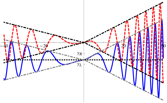
The leading-order behavior in time for (1 2 ± ∞ plus-or-minus \pm\infty [3 ] . In the limit as t → ∞ → 𝑡 t\to\infty x / t 𝑥 𝑡 x/t
q L ( x , t ) ∼ β R γ R σ L + β L γ L σ R β R σ L + β L σ R + e i π 4 − i x 2 4 σ L t 4 σ L t ( β R σ L ( γ R − γ L ) x β R σ L + β L σ L σ R + v ^ 0 L ( − x 2 σ L t ) π − ( β R σ L − β L σ L σ R ) v ^ 0 L ( x 2 σ L t ) ( β R σ L + β L σ L σ R ) π + β R σ L v ^ 0 R ( − x 2 t σ L σ R ) ( β L σ R + β R σ L σ R ) π ) , similar-to superscript 𝑞 𝐿 𝑥 𝑡 subscript 𝛽 𝑅 subscript 𝛾 𝑅 subscript 𝜎 𝐿 subscript 𝛽 𝐿 subscript 𝛾 𝐿 subscript 𝜎 𝑅 subscript 𝛽 𝑅 subscript 𝜎 𝐿 subscript 𝛽 𝐿 subscript 𝜎 𝑅 superscript 𝑒 𝑖 𝜋 4 𝑖 superscript 𝑥 2 4 subscript 𝜎 𝐿 𝑡 4 subscript 𝜎 𝐿 𝑡 subscript 𝛽 𝑅 subscript 𝜎 𝐿 subscript 𝛾 𝑅 subscript 𝛾 𝐿 𝑥 subscript 𝛽 𝑅 subscript 𝜎 𝐿 subscript 𝛽 𝐿 subscript 𝜎 𝐿 subscript 𝜎 𝑅 superscript subscript ^ 𝑣 0 𝐿 𝑥 2 subscript 𝜎 𝐿 𝑡 𝜋 subscript 𝛽 𝑅 subscript 𝜎 𝐿 subscript 𝛽 𝐿 subscript 𝜎 𝐿 subscript 𝜎 𝑅 superscript subscript ^ 𝑣 0 𝐿 𝑥 2 subscript 𝜎 𝐿 𝑡 subscript 𝛽 𝑅 subscript 𝜎 𝐿 subscript 𝛽 𝐿 subscript 𝜎 𝐿 subscript 𝜎 𝑅 𝜋 subscript 𝛽 𝑅 subscript 𝜎 𝐿 superscript subscript ^ 𝑣 0 𝑅 𝑥 2 𝑡 subscript 𝜎 𝐿 subscript 𝜎 𝑅 subscript 𝛽 𝐿 subscript 𝜎 𝑅 subscript 𝛽 𝑅 subscript 𝜎 𝐿 subscript 𝜎 𝑅 𝜋 \begin{split}q^{L}(x,t)&\sim\frac{\beta_{R}\gamma_{R}\sqrt{\sigma_{L}}+\beta_{L}\gamma_{L}\sqrt{\sigma_{R}}}{\beta_{R}\sqrt{\sigma_{L}}+\beta_{L}\sqrt{\sigma_{R}}}+\frac{e^{\frac{i\pi}{4}-\frac{ix^{2}}{4\sigma_{L}t}}}{\sqrt{4\sigma_{L}t}}\left(\frac{\beta_{R}\sigma_{L}(\gamma_{R}-\gamma_{L})x}{\beta_{R}\sigma_{L}+\beta_{L}\sqrt{\sigma_{L}\sigma_{R}}}+\frac{\hat{v}_{0}^{L}\left(-\frac{x}{2\sigma_{L}t}\right)}{\sqrt{\pi}}\right.\\
&\left.-\frac{(\beta_{R}\sigma_{L}-\beta_{L}\sqrt{\sigma_{L}\sigma_{R}})\hat{v}_{0}^{L}\left(\frac{x}{2\sigma_{L}t}\right)}{(\beta_{R}\sigma_{L}+\beta_{L}\sqrt{\sigma_{L}\sigma_{R}})\sqrt{\pi}}+\frac{\beta_{R}\sigma_{L}\hat{v}_{0}^{R}\left(-\frac{x}{2t\sqrt{\sigma_{L}\sigma_{R}}}\right)}{(\beta_{L}\sigma_{R}+\beta_{R}\sqrt{\sigma_{L}\sigma_{R}})\sqrt{\pi}}\right),\end{split} (18)
for − ∞ < x < 0 𝑥 0 -\infty<x<0 0 < x < ∞ 0 𝑥 0<x<\infty
q R ( x , t ) ∼ β R γ R σ L + β L γ L σ R β R σ L + β L σ R + e i π 4 − i x 2 4 σ R t 4 σ R t ( β L σ L σ R ( γ R − γ L ) x β R σ L + β L σ R σ L + v ^ 0 R ( − x 2 σ R t ) π + β L σ R v ^ 0 L ( − x 2 t σ R σ L ) ( β R σ L + β L σ R σ L ) π + ( β R σ L − β L σ L σ R ) v ^ 0 R ( x 2 σ R t ) ( β R σ L + β L σ R σ L ) π ) . similar-to superscript 𝑞 𝑅 𝑥 𝑡 subscript 𝛽 𝑅 subscript 𝛾 𝑅 subscript 𝜎 𝐿 subscript 𝛽 𝐿 subscript 𝛾 𝐿 subscript 𝜎 𝑅 subscript 𝛽 𝑅 subscript 𝜎 𝐿 subscript 𝛽 𝐿 subscript 𝜎 𝑅 superscript 𝑒 𝑖 𝜋 4 𝑖 superscript 𝑥 2 4 subscript 𝜎 𝑅 𝑡 4 subscript 𝜎 𝑅 𝑡 subscript 𝛽 𝐿 subscript 𝜎 𝐿 subscript 𝜎 𝑅 subscript 𝛾 𝑅 subscript 𝛾 𝐿 𝑥 subscript 𝛽 𝑅 subscript 𝜎 𝐿 subscript 𝛽 𝐿 subscript 𝜎 𝑅 subscript 𝜎 𝐿 superscript subscript ^ 𝑣 0 𝑅 𝑥 2 subscript 𝜎 𝑅 𝑡 𝜋 subscript 𝛽 𝐿 subscript 𝜎 𝑅 superscript subscript ^ 𝑣 0 𝐿 𝑥 2 𝑡 subscript 𝜎 𝑅 subscript 𝜎 𝐿 subscript 𝛽 𝑅 subscript 𝜎 𝐿 subscript 𝛽 𝐿 subscript 𝜎 𝑅 subscript 𝜎 𝐿 𝜋 subscript 𝛽 𝑅 subscript 𝜎 𝐿 subscript 𝛽 𝐿 subscript 𝜎 𝐿 subscript 𝜎 𝑅 superscript subscript ^ 𝑣 0 𝑅 𝑥 2 subscript 𝜎 𝑅 𝑡 subscript 𝛽 𝑅 subscript 𝜎 𝐿 subscript 𝛽 𝐿 subscript 𝜎 𝑅 subscript 𝜎 𝐿 𝜋 \begin{split}q^{R}(x,t)&\sim\frac{\beta_{R}\gamma_{R}\sqrt{\sigma_{L}}+\beta_{L}\gamma_{L}\sqrt{\sigma_{R}}}{\beta_{R}\sqrt{\sigma_{L}}+\beta_{L}\sqrt{\sigma_{R}}}+\frac{e^{\frac{i\pi}{4}-\frac{ix^{2}}{4\sigma_{R}t}}}{\sqrt{4\sigma_{R}t}}\left(\frac{\beta_{L}\sqrt{\sigma_{L}\sigma_{R}}(\gamma_{R}-\gamma_{L})x}{\beta_{R}\sigma_{L}+\beta_{L}\sqrt{\sigma_{R}\sigma_{L}}}+\frac{\hat{v}_{0}^{R}\left(-\frac{x}{2\sigma_{R}t}\right)}{\sqrt{\pi}}\right.\\
&\left.+\frac{\beta_{L}\sigma_{R}\hat{v}_{0}^{L}\left(-\frac{x}{2t\sqrt{\sigma_{R}\sigma_{L}}}\right)}{\left(\beta_{R}\sigma_{L}+\beta_{L}\sqrt{\sigma_{R}\sigma_{L}}\right)\sqrt{\pi}}+\frac{(\beta_{R}\sigma_{L}-\beta_{L}\sqrt{\sigma_{L}\sigma_{R}})\hat{v}_{0}^{R}\left(\frac{x}{2\sigma_{R}t}\right)}{\left(\beta_{R}\sigma_{L}+\beta_{L}\sqrt{\sigma_{R}\sigma_{L}}\right)\sqrt{\pi}}\right).\end{split} (19)
The constant factor in (18 19 β R σ L subscript 𝛽 𝑅 subscript 𝜎 𝐿 \beta_{R}\sqrt{\sigma_{L}} β L σ R subscript 𝛽 𝐿 subscript 𝜎 𝑅 \beta_{L}\sqrt{\sigma_{R}} exp ( − i x 2 / ( 4 σ L t ) ) 𝑖 superscript 𝑥 2 4 subscript 𝜎 𝐿 𝑡 \exp(-ix^{2}/(4\sigma_{L}t)) exp ( − i x 2 / ( 4 σ R t ) ) 𝑖 superscript 𝑥 2 4 subscript 𝜎 𝑅 𝑡 \exp(-ix^{2}/(4\sigma_{R}t)) 4 x / t 𝑥 𝑡 x/t x 𝑥 x 4 x / t 𝑥 𝑡 x/t
Figure 4: The leading order behavior of q ( x , t ) 𝑞 𝑥 𝑡 q(x,t) 18 19 t = 10 , γ L = − 20 , γ R = − 10 , β L = 2 , β R = 1 , σ L = 2 formulae-sequence 𝑡 10 formulae-sequence subscript 𝛾 𝐿 20 formulae-sequence subscript 𝛾 𝑅 10 formulae-sequence subscript 𝛽 𝐿 2 formulae-sequence subscript 𝛽 𝑅 1 subscript 𝜎 𝐿 2 t=10,\gamma_{L}=-20,\gamma_{R}=-10,\beta_{L}=2,\beta_{R}=1,\sigma_{L}=2 σ R = 1 subscript 𝜎 𝑅 1 \sigma_{R}=1 q 0 L ( x ) = β L γ L + β R γ R β L + β R + β R γ R − γ L β L + β R tanh ( x ) superscript subscript 𝑞 0 𝐿 𝑥 subscript 𝛽 𝐿 subscript 𝛾 𝐿 subscript 𝛽 𝑅 subscript 𝛾 𝑅 subscript 𝛽 𝐿 subscript 𝛽 𝑅 subscript 𝛽 𝑅 subscript 𝛾 𝑅 subscript 𝛾 𝐿 subscript 𝛽 𝐿 subscript 𝛽 𝑅 𝑥 q_{0}^{L}(x)=\frac{\beta_{L}\gamma_{L}+\beta_{R}\gamma_{R}}{\beta_{L}+\beta_{R}}+\beta_{R}\frac{\gamma_{R}-\gamma_{L}}{\beta_{L}+\beta_{R}}\tanh(x) q 0 R ( x ) = β L γ L + β R γ R β L + β R + β L γ R − γ L β L + β R tanh ( x ) superscript subscript 𝑞 0 𝑅 𝑥 subscript 𝛽 𝐿 subscript 𝛾 𝐿 subscript 𝛽 𝑅 subscript 𝛾 𝑅 subscript 𝛽 𝐿 subscript 𝛽 𝑅 subscript 𝛽 𝐿 subscript 𝛾 𝑅 subscript 𝛾 𝐿 subscript 𝛽 𝐿 subscript 𝛽 𝑅 𝑥 q_{0}^{R}(x)=\frac{\beta_{L}\gamma_{L}+\beta_{R}\gamma_{R}}{\beta_{L}+\beta_{R}}+\beta_{L}\frac{\gamma_{R}-\gamma_{L}}{\beta_{L}+\beta_{R}}\tanh(x)
•
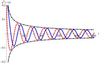
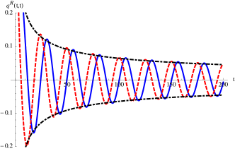
In quantum mechanics one considers only the finite energy case, that is, γ L = 0 = γ R subscript 𝛾 𝐿 0 subscript 𝛾 𝑅 \gamma_{L}=0=\gamma_{R} 5 x / t = ± 1 𝑥 𝑡 plus-or-minus 1 x/t=\pm 1 5
Figure 5: The leading order behavior of q L ( − t , t ) superscript 𝑞 𝐿 𝑡 𝑡 q^{L}(-t,t) q R ( t , t ) superscript 𝑞 𝑅 𝑡 𝑡 q^{R}(t,t) 18 19 γ L = 0 , γ R = 0 , β L = 4 , β R = 1 , σ L = 3 formulae-sequence subscript 𝛾 𝐿 0 formulae-sequence subscript 𝛾 𝑅 0 formulae-sequence subscript 𝛽 𝐿 4 formulae-sequence subscript 𝛽 𝑅 1 subscript 𝜎 𝐿 3 \gamma_{L}=0,\gamma_{R}=0,\beta_{L}=4,\beta_{R}=1,\sigma_{L}=3 σ R = 1 subscript 𝜎 𝑅 1 \sigma_{R}=1 q 0 L ( x ) = ( 1 + β R x ) e − x 2 superscript subscript 𝑞 0 𝐿 𝑥 1 subscript 𝛽 𝑅 𝑥 superscript 𝑒 superscript 𝑥 2 q_{0}^{L}(x)=(1+\beta_{R}x)e^{-x^{2}} q 0 R ( x ) = ( 1 + β L x ) e − x 2 superscript subscript 𝑞 0 𝑅 𝑥 1 subscript 𝛽 𝐿 𝑥 superscript 𝑒 superscript 𝑥 2 q_{0}^{R}(x)=(1+\beta_{L}x)e^{-x^{2}}
3 Two finite domains
We wish to find q L ( x , t ) superscript 𝑞 𝐿 𝑥 𝑡 q^{L}(x,t) q R ( x , t ) superscript 𝑞 𝑅 𝑥 𝑡 q^{R}(x,t)
i q t L ( x , t ) = 𝑖 subscript superscript 𝑞 𝐿 𝑡 𝑥 𝑡 absent \displaystyle iq^{L}_{t}(x,t)= σ L q x x L ( x , t ) subscript 𝜎 𝐿 subscript superscript 𝑞 𝐿 𝑥 𝑥 𝑥 𝑡 \displaystyle\sigma_{L}q^{L}_{xx}(x,t) − a < 𝑎 absent \displaystyle-a< x < 0 , 𝑥 0 \displaystyle x<0, t > 0 , 𝑡 0 \displaystyle t>0, (20)
i q t R ( x , t ) = 𝑖 subscript superscript 𝑞 𝑅 𝑡 𝑥 𝑡 absent \displaystyle iq^{R}_{t}(x,t)= σ R q x x R ( x , t ) subscript 𝜎 𝑅 subscript superscript 𝑞 𝑅 𝑥 𝑥 𝑥 𝑡 \displaystyle\sigma_{R}q^{R}_{xx}(x,t) 0 < 0 absent \displaystyle 0< x < b , 𝑥 𝑏 \displaystyle x<b, t > 0 , 𝑡 0 \displaystyle t>0,
subject to the Robin boundary conditions
α 1 q L ( − a , t ) + α 2 q x L ( − a , t ) = subscript 𝛼 1 superscript 𝑞 𝐿 𝑎 𝑡 subscript 𝛼 2 subscript superscript 𝑞 𝐿 𝑥 𝑎 𝑡 absent \displaystyle\alpha_{1}q^{L}(-a,t)+\alpha_{2}q^{L}_{x}(-a,t)= f L ( t ) , superscript 𝑓 𝐿 𝑡 \displaystyle f^{L}(t),~{}~{} t > 0 , 𝑡 0 \displaystyle t>0, (21)
α 3 q R ( b , t ) + α 4 q x R ( b , t ) = subscript 𝛼 3 superscript 𝑞 𝑅 𝑏 𝑡 subscript 𝛼 4 subscript superscript 𝑞 𝑅 𝑥 𝑏 𝑡 absent \displaystyle\alpha_{3}q^{R}(b,t)+\alpha_{4}q^{R}_{x}(b,t)= f R ( t ) , superscript 𝑓 𝑅 𝑡 \displaystyle f^{R}(t),~{}~{} t > 0 , 𝑡 0 \displaystyle t>0,
the initial conditions
q L ( x , 0 ) = superscript 𝑞 𝐿 𝑥 0 absent \displaystyle q^{L}(x,0)= q 0 L ( x ) , subscript superscript 𝑞 𝐿 0 𝑥 \displaystyle q^{L}_{0}(x),~{}~{}~{} − a < 𝑎 absent \displaystyle-a< x < 0 , 𝑥 0 \displaystyle x<0, (22)
q R ( x , 0 ) = superscript 𝑞 𝑅 𝑥 0 absent \displaystyle q^{R}(x,0)= q 0 R ( x ) , subscript superscript 𝑞 𝑅 0 𝑥 \displaystyle q^{R}_{0}(x),~{}~{}~{} 0 < 0 absent \displaystyle 0< x < b , 𝑥 𝑏 \displaystyle x<b,
and the interface conditions
q L ( 0 , t ) = superscript 𝑞 𝐿 0 𝑡 absent \displaystyle q^{L}(0,t)= q R ( 0 , t ) , superscript 𝑞 𝑅 0 𝑡 \displaystyle q^{R}(0,t),~{}~{} t > 0 , 𝑡 0 \displaystyle t>0, (23)
β L q x L ( 0 , t ) = subscript 𝛽 𝐿 subscript superscript 𝑞 𝐿 𝑥 0 𝑡 absent \displaystyle\beta_{L}q^{L}_{x}(0,t)= β R q x R ( 0 , t ) , subscript 𝛽 𝑅 subscript superscript 𝑞 𝑅 𝑥 0 𝑡 \displaystyle\beta_{R}q^{R}_{x}(0,t),~{}~{} t > 0 , 𝑡 0 \displaystyle t>0,
where a > 0 𝑎 0 a>0 b > 0 𝑏 0 b>0 β L subscript 𝛽 𝐿 \beta_{L} β R subscript 𝛽 𝑅 \beta_{R} α i subscript 𝛼 𝑖 \alpha_{i} 1 ≤ i ≤ 4 1 𝑖 4 1\leq i\leq 4 t 𝑡 t σ L subscript 𝜎 𝐿 \sigma_{L} σ R subscript 𝜎 𝑅 \sigma_{R} α 1 = α 3 = 0 subscript 𝛼 1 subscript 𝛼 3 0 \alpha_{1}=\alpha_{3}=0 α 2 = α 4 = 0 subscript 𝛼 2 subscript 𝛼 4 0 \alpha_{2}=\alpha_{4}=0
As before we begin with the local relations
( e − i k x + λ L t q L ( x , t ) ) t = subscript superscript 𝑒 𝑖 𝑘 𝑥 subscript 𝜆 𝐿 𝑡 superscript 𝑞 𝐿 𝑥 𝑡 𝑡 absent \displaystyle\left(e^{-ikx+{\color[rgb]{0,0,0}\lambda_{L}}t}q^{L}(x,t)\right)_{t}= ( σ L e − i k x + λ L t ( k q L ( x , t ) − i q x L ( x , t ) ) ) x , subscript subscript 𝜎 𝐿 superscript 𝑒 𝑖 𝑘 𝑥 subscript 𝜆 𝐿 𝑡 𝑘 superscript 𝑞 𝐿 𝑥 𝑡 𝑖 subscript superscript 𝑞 𝐿 𝑥 𝑥 𝑡 𝑥 \displaystyle\left(\sigma_{L}e^{-ikx+{\color[rgb]{0,0,0}\lambda_{L}}t}(kq^{L}(x,t)-iq^{L}_{x}(x,t))\right)_{x}, (24a)
( e − i k x + λ R t q L ( x , t ) ) t = subscript superscript 𝑒 𝑖 𝑘 𝑥 subscript 𝜆 𝑅 𝑡 superscript 𝑞 𝐿 𝑥 𝑡 𝑡 absent \displaystyle\left(e^{-ikx+{\color[rgb]{0,0,0}\lambda_{R}}t}q^{L}(x,t)\right)_{t}= ( σ R e − i k x + λ R t ( k q R ( x , t ) − i q x R ( x , t ) ) ) x . subscript subscript 𝜎 𝑅 superscript 𝑒 𝑖 𝑘 𝑥 subscript 𝜆 𝑅 𝑡 𝑘 superscript 𝑞 𝑅 𝑥 𝑡 𝑖 subscript superscript 𝑞 𝑅 𝑥 𝑥 𝑡 𝑥 \displaystyle\left(\sigma_{R}e^{-ikx+{\color[rgb]{0,0,0}\lambda_{R}}t}(kq^{R}(x,t)-iq^{R}_{x}(x,t))\right)_{x}. (24b)
For k ∈ ℂ 𝑘 ℂ k\in\mathbb{C}
f ^ L ( ω , t ) = subscript ^ 𝑓 𝐿 𝜔 𝑡 absent \displaystyle\hat{f}_{L}(\omega,t)= ∫ 0 t e ω s f L ( s ) d s , superscript subscript 0 𝑡 superscript 𝑒 𝜔 𝑠 subscript 𝑓 𝐿 𝑠 differential-d 𝑠 \displaystyle\int_{0}^{t}e^{\omega s}f_{L}(s)\,\mathrm{d}s, f ^ R ( ω , t ) = subscript ^ 𝑓 𝑅 𝜔 𝑡 absent \displaystyle\hat{f}_{R}(\omega,t)= ∫ 0 t e ω s f R ( s ) d s , superscript subscript 0 𝑡 superscript 𝑒 𝜔 𝑠 subscript 𝑓 𝑅 𝑠 differential-d 𝑠 \displaystyle\int_{0}^{t}e^{\omega s}f_{R}(s)\,\mathrm{d}s,
h 1 L ( ω , t ) = superscript subscript ℎ 1 𝐿 𝜔 𝑡 absent \displaystyle h_{1}^{L}(\omega,t)= ∫ 0 t e ω s q x L ( − a , s ) d s , superscript subscript 0 𝑡 superscript 𝑒 𝜔 𝑠 subscript superscript 𝑞 𝐿 𝑥 𝑎 𝑠 differential-d 𝑠 \displaystyle\int_{0}^{t}e^{\omega s}q^{L}_{x}(-a,s)\,\mathrm{d}s, h 0 L ( ω , t ) = superscript subscript ℎ 0 𝐿 𝜔 𝑡 absent \displaystyle h_{0}^{L}(\omega,t)= ∫ 0 t e ω s q L ( − a , s ) d s , superscript subscript 0 𝑡 superscript 𝑒 𝜔 𝑠 superscript 𝑞 𝐿 𝑎 𝑠 differential-d 𝑠 \displaystyle\int_{0}^{t}e^{\omega s}q^{L}(-a,s)\,\mathrm{d}s,
h 1 R ( ω , t ) = superscript subscript ℎ 1 𝑅 𝜔 𝑡 absent \displaystyle h_{1}^{R}(\omega,t)= ∫ 0 t e ω s q x R ( b , s ) d s , superscript subscript 0 𝑡 superscript 𝑒 𝜔 𝑠 subscript superscript 𝑞 𝑅 𝑥 𝑏 𝑠 differential-d 𝑠 \displaystyle\int_{0}^{t}e^{\omega s}q^{R}_{x}(b,s)\,\mathrm{d}s, h 0 R ( ω , t ) = superscript subscript ℎ 0 𝑅 𝜔 𝑡 absent \displaystyle h_{0}^{R}(\omega,t)= ∫ 0 t e ω s q R ( b , s ) d s , superscript subscript 0 𝑡 superscript 𝑒 𝜔 𝑠 superscript 𝑞 𝑅 𝑏 𝑠 differential-d 𝑠 \displaystyle\int_{0}^{t}e^{\omega s}q^{R}(b,s)\,\mathrm{d}s,
q ^ L ( k , t ) = superscript ^ 𝑞 𝐿 𝑘 𝑡 absent \displaystyle\hat{q}^{L}(k,t)= ∫ − a 0 e − i k x q L ( x , t ) d x , superscript subscript 𝑎 0 superscript 𝑒 𝑖 𝑘 𝑥 superscript 𝑞 𝐿 𝑥 𝑡 differential-d 𝑥 \displaystyle\int_{-a}^{0}e^{-ikx}q^{L}(x,t)\,\mathrm{d}x, q ^ 0 L ( k ) = subscript superscript ^ 𝑞 𝐿 0 𝑘 absent \displaystyle\hat{q}^{L}_{0}(k)= ∫ − a 0 e − i k x q 0 L ( x ) d x , superscript subscript 𝑎 0 superscript 𝑒 𝑖 𝑘 𝑥 subscript superscript 𝑞 𝐿 0 𝑥 differential-d 𝑥 \displaystyle\int_{-a}^{0}e^{-ikx}q^{L}_{0}(x)\,\mathrm{d}x,
q ^ R ( k , t ) = superscript ^ 𝑞 𝑅 𝑘 𝑡 absent \displaystyle\hat{q}^{R}(k,t)= ∫ 0 b e − i k x q R ( x , t ) d x , superscript subscript 0 𝑏 superscript 𝑒 𝑖 𝑘 𝑥 superscript 𝑞 𝑅 𝑥 𝑡 differential-d 𝑥 \displaystyle\int_{0}^{b}e^{-ikx}q^{R}(x,t)\,\mathrm{d}x, q ^ 0 R ( k ) = subscript superscript ^ 𝑞 𝑅 0 𝑘 absent \displaystyle\hat{q}^{R}_{0}(k)= ∫ 0 b e − i k x q 0 R ( x ) d x , superscript subscript 0 𝑏 superscript 𝑒 𝑖 𝑘 𝑥 subscript superscript 𝑞 𝑅 0 𝑥 differential-d 𝑥 \displaystyle\int_{0}^{b}e^{-ikx}q^{R}_{0}(x)\,\mathrm{d}x,
g 0 ( ω , t ) = subscript 𝑔 0 𝜔 𝑡 absent \displaystyle g_{0}({\omega},t)= ∫ 0 t e ω s q L ( 0 , s ) d s = ∫ 0 t e ω s q R ( 0 , s ) d s , superscript subscript 0 𝑡 superscript 𝑒 𝜔 𝑠 superscript 𝑞 𝐿 0 𝑠 differential-d 𝑠 superscript subscript 0 𝑡 superscript 𝑒 𝜔 𝑠 superscript 𝑞 𝑅 0 𝑠 differential-d 𝑠 \displaystyle\int_{0}^{t}e^{\omega s}q^{L}(0,s)\,\mathrm{d}s=\int_{0}^{t}e^{\omega s}q^{R}(0,s)\,\mathrm{d}s,
g 1 ( ω , t ) = subscript 𝑔 1 𝜔 𝑡 absent \displaystyle g_{1}({\omega},t)= ∫ 0 t e ω s q x L ( 0 , s ) d s = β R β L ∫ 0 t e ω s q x R ( 0 , s ) d s . superscript subscript 0 𝑡 superscript 𝑒 𝜔 𝑠 subscript superscript 𝑞 𝐿 𝑥 0 𝑠 differential-d 𝑠 subscript 𝛽 𝑅 subscript 𝛽 𝐿 superscript subscript 0 𝑡 superscript 𝑒 𝜔 𝑠 subscript superscript 𝑞 𝑅 𝑥 0 𝑠 differential-d 𝑠 \displaystyle\int_{0}^{t}e^{{\omega}s}q^{L}_{x}(0,s)\,\mathrm{d}s=\frac{\beta_{R}}{\beta_{L}}\int_{0}^{t}e^{{\omega}s}q^{R}_{x}(0,s)\,\mathrm{d}s.
Applying Green’s Theorem [1 ] in the domains [ − a , 0 ] × [ 0 , t ] 𝑎 0 0 𝑡 [-a,0]\times[0,t] [ 0 , b ] × [ 0 , t ] 0 𝑏 0 𝑡 [0,b]\times[0,t]
e λ L t q ^ L ( k , t ) = superscript 𝑒 subscript 𝜆 𝐿 𝑡 superscript ^ 𝑞 𝐿 𝑘 𝑡 absent \displaystyle e^{{\color[rgb]{0,0,0}\lambda_{L}}t}\hat{q}^{L}(k,t)= q ^ 0 L ( k ) + k σ L g 0 ( λ L , t ) − i σ L g 1 ( λ L , t ) − σ L e i k a ( k h 0 L ( λ L , t ) − i h 1 L ( λ L , t ) ) , superscript subscript ^ 𝑞 0 𝐿 𝑘 𝑘 subscript 𝜎 𝐿 subscript 𝑔 0 subscript 𝜆 𝐿 𝑡 𝑖 subscript 𝜎 𝐿 subscript 𝑔 1 subscript 𝜆 𝐿 𝑡 subscript 𝜎 𝐿 superscript 𝑒 𝑖 𝑘 𝑎 𝑘 superscript subscript ℎ 0 𝐿 subscript 𝜆 𝐿 𝑡 𝑖 superscript subscript ℎ 1 𝐿 subscript 𝜆 𝐿 𝑡 \displaystyle\hat{q}_{0}^{L}(k)+k\sigma_{L}g_{0}({\color[rgb]{0,0,0}\lambda_{L}},t)-i\sigma_{L}g_{1}({\color[rgb]{0,0,0}\lambda_{L}},t)-\sigma_{L}e^{ika}(kh_{0}^{L}({\color[rgb]{0,0,0}\lambda_{L}},t)-ih_{1}^{L}({\color[rgb]{0,0,0}\lambda_{L}},t)), (25a)
e λ R t q ^ R ( k , t ) = superscript 𝑒 subscript 𝜆 𝑅 𝑡 superscript ^ 𝑞 𝑅 𝑘 𝑡 absent \displaystyle e^{{\color[rgb]{0,0,0}\lambda_{R}}t}\hat{q}^{R}(k,t)= q ^ 0 R ( k ) − k σ R g 0 ( λ R , t ) + i σ R β L β R g 1 ( λ R , t ) + σ R e − i k b ( k h 0 R ( λ R , t ) − i h 1 R ( λ R , t ) ) , superscript subscript ^ 𝑞 0 𝑅 𝑘 𝑘 subscript 𝜎 𝑅 subscript 𝑔 0 subscript 𝜆 𝑅 𝑡 𝑖 subscript 𝜎 𝑅 subscript 𝛽 𝐿 subscript 𝛽 𝑅 subscript 𝑔 1 subscript 𝜆 𝑅 𝑡 subscript 𝜎 𝑅 superscript 𝑒 𝑖 𝑘 𝑏 𝑘 superscript subscript ℎ 0 𝑅 subscript 𝜆 𝑅 𝑡 𝑖 superscript subscript ℎ 1 𝑅 subscript 𝜆 𝑅 𝑡 \displaystyle\hat{q}_{0}^{R}(k)-k\sigma_{R}g_{0}({\color[rgb]{0,0,0}\lambda_{R}},t)+\frac{i\sigma_{R}\beta_{L}}{\beta_{R}}g_{1}({\color[rgb]{0,0,0}\lambda_{R}},t)+\sigma_{R}e^{-ikb}(kh_{0}^{R}({\color[rgb]{0,0,0}\lambda_{R}},t)-ih_{1}^{R}({\color[rgb]{0,0,0}\lambda_{R}},t)), (25b)
which are valid for all k ∈ ℂ 𝑘 ℂ k\in\mathbb{C} 7 λ L ( k ) subscript 𝜆 𝐿 𝑘 {\color[rgb]{0,0,0}\lambda_{L}}(k) λ R ( k ) subscript 𝜆 𝑅 𝑘 {\color[rgb]{0,0,0}\lambda_{R}}(k) k → − k → 𝑘 𝑘 k\to-k 25 − k 𝑘 -k
e λ L t q ^ L ( − k , t ) = superscript 𝑒 subscript 𝜆 𝐿 𝑡 superscript ^ 𝑞 𝐿 𝑘 𝑡 absent \displaystyle e^{{\color[rgb]{0,0,0}\lambda_{L}}t}\hat{q}^{L}(-k,t)= q ^ 0 L ( − k ) − k σ L g 0 ( λ L , t ) − i σ L g 1 ( λ L , t ) − σ L e − i k a ( − k h 0 L ( λ L , t ) − i h 1 L ( λ L , t ) ) , superscript subscript ^ 𝑞 0 𝐿 𝑘 𝑘 subscript 𝜎 𝐿 subscript 𝑔 0 subscript 𝜆 𝐿 𝑡 𝑖 subscript 𝜎 𝐿 subscript 𝑔 1 subscript 𝜆 𝐿 𝑡 subscript 𝜎 𝐿 superscript 𝑒 𝑖 𝑘 𝑎 𝑘 superscript subscript ℎ 0 𝐿 subscript 𝜆 𝐿 𝑡 𝑖 superscript subscript ℎ 1 𝐿 subscript 𝜆 𝐿 𝑡 \displaystyle\hat{q}_{0}^{L}(-k)-k\sigma_{L}g_{0}({\color[rgb]{0,0,0}\lambda_{L}},t)-i\sigma_{L}g_{1}({\color[rgb]{0,0,0}\lambda_{L}},t)-\sigma_{L}e^{-ika}(-kh_{0}^{L}({\color[rgb]{0,0,0}\lambda_{L}},t)-ih_{1}^{L}({\color[rgb]{0,0,0}\lambda_{L}},t)), (26a)
e λ R t q ^ R ( − k , t ) = superscript 𝑒 subscript 𝜆 𝑅 𝑡 superscript ^ 𝑞 𝑅 𝑘 𝑡 absent \displaystyle e^{{\color[rgb]{0,0,0}\lambda_{R}}t}\hat{q}^{R}(-k,t)= q ^ 0 R ( − k ) + k σ R g 0 ( λ R , t ) + i σ R β L β R g 1 ( λ R , t ) + σ R e i k b ( − k h 0 R ( λ R , t ) − i h 1 R ( λ R , t ) ) , superscript subscript ^ 𝑞 0 𝑅 𝑘 𝑘 subscript 𝜎 𝑅 subscript 𝑔 0 subscript 𝜆 𝑅 𝑡 𝑖 subscript 𝜎 𝑅 subscript 𝛽 𝐿 subscript 𝛽 𝑅 subscript 𝑔 1 subscript 𝜆 𝑅 𝑡 subscript 𝜎 𝑅 superscript 𝑒 𝑖 𝑘 𝑏 𝑘 superscript subscript ℎ 0 𝑅 subscript 𝜆 𝑅 𝑡 𝑖 superscript subscript ℎ 1 𝑅 subscript 𝜆 𝑅 𝑡 \displaystyle\hat{q}_{0}^{R}(-k)+k\sigma_{R}g_{0}({\color[rgb]{0,0,0}\lambda_{R}},t)+\frac{i\sigma_{R}\beta_{L}}{\beta_{R}}g_{1}({\color[rgb]{0,0,0}\lambda_{R}},t)+\sigma_{R}e^{ikb}(-kh_{0}^{R}({\color[rgb]{0,0,0}\lambda_{R}},t)-ih_{1}^{R}({\color[rgb]{0,0,0}\lambda_{R}},t)), (26b)
Inverting the Fourier transform in (25a
q L ( x , t ) = superscript 𝑞 𝐿 𝑥 𝑡 absent \displaystyle q^{L}(x,t)= 1 2 π ∫ − ∞ ∞ e i k x − λ L t q ^ 0 L ( k ) d k + 1 2 π ∫ − ∞ ∞ e i k x − λ L t σ L ( k g 0 ( λ L , t ) − i g 1 ( λ L , t ) ) d k 1 2 𝜋 superscript subscript superscript 𝑒 𝑖 𝑘 𝑥 subscript 𝜆 𝐿 𝑡 superscript subscript ^ 𝑞 0 𝐿 𝑘 differential-d 𝑘 1 2 𝜋 superscript subscript superscript 𝑒 𝑖 𝑘 𝑥 subscript 𝜆 𝐿 𝑡 subscript 𝜎 𝐿 𝑘 subscript 𝑔 0 subscript 𝜆 𝐿 𝑡 𝑖 subscript 𝑔 1 subscript 𝜆 𝐿 𝑡 differential-d 𝑘 \displaystyle\frac{1}{2\pi}\int_{-\infty}^{\infty}e^{ikx-{\color[rgb]{0,0,0}\lambda_{L}}t}\hat{q}_{0}^{L}(k)\,\mathrm{d}k+\frac{1}{2\pi}\int_{-\infty}^{\infty}e^{ikx-{\color[rgb]{0,0,0}\lambda_{L}}t}\sigma_{L}(kg_{0}({\color[rgb]{0,0,0}\lambda_{L}},t)-ig_{1}({\color[rgb]{0,0,0}\lambda_{L}},t))\,\mathrm{d}k
+ 1 2 π ∫ − ∞ ∞ σ L e i k ( x + a ) − λ L t ( k h 0 L ( λ L , t ) − i h 1 L ( λ L , t ) ) d k , 1 2 𝜋 superscript subscript subscript 𝜎 𝐿 superscript 𝑒 𝑖 𝑘 𝑥 𝑎 subscript 𝜆 𝐿 𝑡 𝑘 superscript subscript ℎ 0 𝐿 subscript 𝜆 𝐿 𝑡 𝑖 superscript subscript ℎ 1 𝐿 subscript 𝜆 𝐿 𝑡 differential-d 𝑘 \displaystyle+\frac{1}{2\pi}\int_{-\infty}^{\infty}\sigma_{L}e^{ik(x+a)-{\color[rgb]{0,0,0}\lambda_{L}}t}(kh_{0}^{L}({\color[rgb]{0,0,0}\lambda_{L}},t)-ih_{1}^{L}({\color[rgb]{0,0,0}\lambda_{L}},t))\,\mathrm{d}k,
for − a < x < 0 𝑎 𝑥 0 -a<x<0 t > 0 𝑡 0 t>0 k → ∞ → 𝑘 k\to\infty k ∈ ℂ − ∖ D − 𝑘 superscript ℂ superscript 𝐷 k\in\mathbb{C}^{-}\setminus D^{-} k → ∞ → 𝑘 k\to\infty k ∈ ℂ + ∖ D + 𝑘 superscript ℂ superscript 𝐷 k\in\mathbb{C}^{+}\setminus D^{+} D + superscript 𝐷 D^{+} D 0 + subscript superscript 𝐷 0 D^{+}_{0} D − superscript 𝐷 D^{-} D 0 − subscript superscript 𝐷 0 D^{-}_{0} 6
q L ( x , t ) = 1 2 π ∫ − ∞ ∞ e i k x − λ L t q ^ 0 L ( k ) d k − 1 2 π ∫ ∂ D 0 − e i k x − λ L t σ L ( k g 0 ( λ L , t ) − i g 1 ( λ L , t ) ) d k + 1 2 π ∫ ∂ D 0 + σ L e i k ( x + a ) − λ L t ( k h 0 L ( λ L , t ) − i h 1 L ( λ L , t ) ) d k . superscript 𝑞 𝐿 𝑥 𝑡 1 2 𝜋 superscript subscript superscript 𝑒 𝑖 𝑘 𝑥 subscript 𝜆 𝐿 𝑡 superscript subscript ^ 𝑞 0 𝐿 𝑘 differential-d 𝑘 1 2 𝜋 subscript superscript subscript 𝐷 0 superscript 𝑒 𝑖 𝑘 𝑥 subscript 𝜆 𝐿 𝑡 subscript 𝜎 𝐿 𝑘 subscript 𝑔 0 subscript 𝜆 𝐿 𝑡 𝑖 subscript 𝑔 1 subscript 𝜆 𝐿 𝑡 differential-d 𝑘 1 2 𝜋 subscript superscript subscript 𝐷 0 subscript 𝜎 𝐿 superscript 𝑒 𝑖 𝑘 𝑥 𝑎 subscript 𝜆 𝐿 𝑡 𝑘 superscript subscript ℎ 0 𝐿 subscript 𝜆 𝐿 𝑡 𝑖 superscript subscript ℎ 1 𝐿 subscript 𝜆 𝐿 𝑡 differential-d 𝑘 \begin{split}q^{L}(x,t)=&\frac{1}{2\pi}\int_{-\infty}^{\infty}e^{ikx-{\color[rgb]{0,0,0}\lambda_{L}}t}\hat{q}_{0}^{L}(k)\,\mathrm{d}k-\frac{1}{2\pi}\int_{\partial D_{0}^{-}}e^{ikx-{\color[rgb]{0,0,0}\lambda_{L}}t}\sigma_{L}(kg_{0}({\color[rgb]{0,0,0}\lambda_{L}},t)-ig_{1}({\color[rgb]{0,0,0}\lambda_{L}},t))\,\mathrm{d}k\\
&+\frac{1}{2\pi}\int_{\partial D_{0}^{+}}\sigma_{L}e^{ik(x+a)-{\color[rgb]{0,0,0}\lambda_{L}}t}(kh_{0}^{L}({\color[rgb]{0,0,0}\lambda_{L}},t)-ih_{1}^{L}({\color[rgb]{0,0,0}\lambda_{L}},t))\,\mathrm{d}k.\end{split} (27)
Im ( k ) Im 𝑘 \operatorname{Im}(k)
Re ( k ) Re 𝑘 \operatorname{Re}(k)
D 0 + superscript subscript 𝐷 0 D_{0}^{+}
D 0 − superscript subscript 𝐷 0 D_{0}^{-}
Figure 6: Deformation of the contours in Figure 2
Similarly, inverting the Fourier transform in (25b
q R ( x , t ) = 1 2 π ∫ − ∞ ∞ e i k x − λ R t q ^ 0 R ( k ) d k + 1 2 π ∫ − ∞ ∞ e i k x − λ R t σ R ( − k g 0 ( λ R , t ) + i β L β R g 1 ( λ R , t ) ) d k + 1 2 π ∫ − ∞ ∞ e i k ( x − b ) − λ R t σ R ( k h 0 R ( λ R , t ) − i h 1 R ( λ R , t ) ) d k , superscript 𝑞 𝑅 𝑥 𝑡 1 2 𝜋 superscript subscript superscript 𝑒 𝑖 𝑘 𝑥 subscript 𝜆 𝑅 𝑡 superscript subscript ^ 𝑞 0 𝑅 𝑘 differential-d 𝑘 1 2 𝜋 superscript subscript superscript 𝑒 𝑖 𝑘 𝑥 subscript 𝜆 𝑅 𝑡 subscript 𝜎 𝑅 𝑘 subscript 𝑔 0 subscript 𝜆 𝑅 𝑡 𝑖 subscript 𝛽 𝐿 subscript 𝛽 𝑅 subscript 𝑔 1 subscript 𝜆 𝑅 𝑡 differential-d 𝑘 1 2 𝜋 superscript subscript superscript 𝑒 𝑖 𝑘 𝑥 𝑏 subscript 𝜆 𝑅 𝑡 subscript 𝜎 𝑅 𝑘 superscript subscript ℎ 0 𝑅 subscript 𝜆 𝑅 𝑡 𝑖 superscript subscript ℎ 1 𝑅 subscript 𝜆 𝑅 𝑡 differential-d 𝑘 \begin{split}q^{R}(x,t)=&\frac{1}{2\pi}\int_{-\infty}^{\infty}e^{ikx-{\color[rgb]{0,0,0}\lambda_{R}}t}\hat{q}_{0}^{R}(k)\,\mathrm{d}k+\frac{1}{2\pi}\int_{-\infty}^{\infty}e^{ikx-{\color[rgb]{0,0,0}\lambda_{R}}t}\sigma_{R}\left(-kg_{0}({\color[rgb]{0,0,0}\lambda_{R}},t)+\frac{i\beta_{L}}{\beta_{R}}g_{1}({\color[rgb]{0,0,0}\lambda_{R}},t)\right)\,\mathrm{d}k\\
&+\frac{1}{2\pi}\int_{-\infty}^{\infty}e^{ik(x-b)-{\color[rgb]{0,0,0}\lambda_{R}}t}\sigma_{R}(kh_{0}^{R}({\color[rgb]{0,0,0}\lambda_{R}},t)-ih_{1}^{R}({\color[rgb]{0,0,0}\lambda_{R}},t))\,\mathrm{d}k,\end{split}
for 0 < x < b 0 𝑥 𝑏 0<x<b t > 0 𝑡 0 t>0 k → ∞ → 𝑘 k\to\infty k ∈ ℂ + ∖ D + 𝑘 superscript ℂ superscript 𝐷 k\in\mathbb{C}^{+}\setminus D^{+} k → ∞ → 𝑘 k\to\infty k ∈ ℂ − ∖ D − 𝑘 superscript ℂ superscript 𝐷 k\in\mathbb{C}^{-}\setminus D^{-}
q R ( x , t ) = 1 2 π ∫ − ∞ ∞ e i k x − λ R t q ^ 0 R ( k ) d k + 1 2 π ∫ ∂ D 0 + e i k x − λ R t σ R ( − k g 0 ( λ R , t ) + i β L β R g 1 ( λ R , t ) ) d k − 1 2 π ∫ ∂ D 0 − e i k ( x − b ) − λ R t σ R ( k h 0 R ( λ R , t ) − i h 1 R ( λ R , t ) ) d k . superscript 𝑞 𝑅 𝑥 𝑡 1 2 𝜋 superscript subscript superscript 𝑒 𝑖 𝑘 𝑥 subscript 𝜆 𝑅 𝑡 superscript subscript ^ 𝑞 0 𝑅 𝑘 differential-d 𝑘 1 2 𝜋 subscript superscript subscript 𝐷 0 superscript 𝑒 𝑖 𝑘 𝑥 subscript 𝜆 𝑅 𝑡 subscript 𝜎 𝑅 𝑘 subscript 𝑔 0 subscript 𝜆 𝑅 𝑡 𝑖 subscript 𝛽 𝐿 subscript 𝛽 𝑅 subscript 𝑔 1 subscript 𝜆 𝑅 𝑡 differential-d 𝑘 1 2 𝜋 subscript superscript subscript 𝐷 0 superscript 𝑒 𝑖 𝑘 𝑥 𝑏 subscript 𝜆 𝑅 𝑡 subscript 𝜎 𝑅 𝑘 superscript subscript ℎ 0 𝑅 subscript 𝜆 𝑅 𝑡 𝑖 superscript subscript ℎ 1 𝑅 subscript 𝜆 𝑅 𝑡 differential-d 𝑘 \begin{split}q^{R}(x,t)=&\frac{1}{2\pi}\int_{-\infty}^{\infty}e^{ikx-{\color[rgb]{0,0,0}\lambda_{R}}t}\hat{q}_{0}^{R}(k)\,\mathrm{d}k+\frac{1}{2\pi}\int_{\partial D_{0}^{+}}e^{ikx-{\color[rgb]{0,0,0}\lambda_{R}}t}\sigma_{R}\left(-kg_{0}({\color[rgb]{0,0,0}\lambda_{R}},t)+\frac{i\beta_{L}}{\beta_{R}}g_{1}({\color[rgb]{0,0,0}\lambda_{R}},t)\right)\,\mathrm{d}k\\
&-\frac{1}{2\pi}\int_{\partial D_{0}^{-}}e^{ik(x-b)-{\color[rgb]{0,0,0}\lambda_{R}}t}\sigma_{R}(kh_{0}^{R}({\color[rgb]{0,0,0}\lambda_{R}},t)-ih_{1}^{R}({\color[rgb]{0,0,0}\lambda_{R}},t))\,\mathrm{d}k.\end{split} (28)
Taking the time transform of the boundary conditions results in
α 1 h 0 L ( ω , t ) + α 2 h 1 L ( ω , t ) = f ^ L ( ω , t ) , subscript 𝛼 1 superscript subscript ℎ 0 𝐿 𝜔 𝑡 subscript 𝛼 2 superscript subscript ℎ 1 𝐿 𝜔 𝑡 superscript ^ 𝑓 𝐿 𝜔 𝑡 \alpha_{1}h_{0}^{L}(\omega,t)+\alpha_{2}h_{1}^{L}(\omega,t)=\hat{f}^{L}(\omega,t), (29)
and
α 3 h 0 R ( ω , t ) + α 4 h 1 R ( ω , t ) = f ^ R ( ω , t ) . subscript 𝛼 3 superscript subscript ℎ 0 𝑅 𝜔 𝑡 subscript 𝛼 4 superscript subscript ℎ 1 𝑅 𝜔 𝑡 superscript ^ 𝑓 𝑅 𝜔 𝑡 \alpha_{3}h_{0}^{R}(\omega,t)+\alpha_{4}h_{1}^{R}(\omega,t)=\hat{f}^{R}(\omega,t). (30)
To obtain a system of six equations for the six unknown functions g 0 ( ω , t ) subscript 𝑔 0 𝜔 𝑡 g_{0}(\omega,t) g 1 ( ω , t ) subscript 𝑔 1 𝜔 𝑡 g_{1}(\omega,t) h 0 L ( ω , t ) superscript subscript ℎ 0 𝐿 𝜔 𝑡 h_{0}^{L}(\omega,t) h 1 L ( ω , t ) superscript subscript ℎ 1 𝐿 𝜔 𝑡 h_{1}^{L}(\omega,t) h 0 R ( ω , t ) superscript subscript ℎ 0 𝑅 𝜔 𝑡 h_{0}^{R}(\omega,t) h 1 R ( ω , t ) superscript subscript ℎ 1 𝑅 𝜔 𝑡 h_{1}^{R}(\omega,t) k 𝑘 k − k 𝑘 -k 25 26 29 30
Although we could solve this problem in its full generality, we restrict to the case of Dirichlet boundary conditions (α 2 = α 4 = 0 subscript 𝛼 2 subscript 𝛼 4 0 \alpha_{2}=\alpha_{4}=0 h 1 L ( ω , t ) superscript subscript ℎ 1 𝐿 𝜔 𝑡 h_{1}^{L}(\omega,t) h 1 R ( ω , t ) superscript subscript ℎ 1 𝑅 𝜔 𝑡 h_{1}^{R}(\omega,t) Δ L ( k ) = 0 subscript Δ 𝐿 𝑘 0 \Delta_{L}(k)=0
Δ L ( k ) = 4 i π α 1 α 3 σ R e i k ( a + b σ L σ R ) ( β L cos ( a k ) sin ( b k σ L σ R ) + β R σ L σ R sin ( a k ) cos ( b k σ L σ R ) ) . subscript Δ 𝐿 𝑘 4 𝑖 𝜋 subscript 𝛼 1 subscript 𝛼 3 subscript 𝜎 𝑅 superscript 𝑒 𝑖 𝑘 𝑎 𝑏 subscript 𝜎 𝐿 subscript 𝜎 𝑅 subscript 𝛽 𝐿 𝑎 𝑘 𝑏 𝑘 subscript 𝜎 𝐿 subscript 𝜎 𝑅 subscript 𝛽 𝑅 subscript 𝜎 𝐿 subscript 𝜎 𝑅 𝑎 𝑘 𝑏 𝑘 subscript 𝜎 𝐿 subscript 𝜎 𝑅 \Delta_{L}(k)=4i\pi\alpha_{1}\alpha_{3}\sigma_{R}e^{ik\left(a+b\sqrt{\frac{\sigma_{L}}{\sigma_{R}}}\right)}\left(\beta_{L}\cos(ak)\sin\left(bk\sqrt{\frac{\sigma_{L}}{\sigma_{R}}}\right)+\beta_{R}\sqrt{\frac{\sigma_{L}}{\sigma_{R}}}\sin(ak)\cos\left(bk\sqrt{\frac{\sigma_{L}}{\sigma_{R}}}\right)\right). (31)
It is easily seen that all values of k 𝑘 k k = 0 𝑘 0 k=0 q ^ L ( k , t ) superscript ^ 𝑞 𝐿 𝑘 𝑡 \hat{q}^{L}(k,t) q ^ R ( k , t ) superscript ^ 𝑞 𝑅 𝑘 𝑡 \hat{q}^{R}(k,t) K L ( x , t ) superscript 𝐾 𝐿 𝑥 𝑡 K^{L}(x,t) K R ( x , t ) superscript 𝐾 𝑅 𝑥 𝑡 K^{R}(x,t) 2
q L ( x , t ) = K L ( x , t ) − ∫ ∂ D 0 − α 1 α 3 σ R 2 Δ L ( k ) e i k x ( β L ( e 2 i b k σ L σ R − 1 ) − β R σ L σ R ( e 2 i b k σ L σ R + 1 ) ) q ^ L ( k , t ) d k + ∫ ∂ D 0 − α 1 α 3 σ R 2 Δ L ( k ) e i k ( 2 a + x ) ( β L ( e 2 i b k σ L σ R − 1 ) − β R σ L σ R ( e 2 i b k σ L σ R + 1 ) ) q ^ L ( − k , t ) d k + ∫ ∂ D 0 − α 1 α 3 β R σ L Δ L ( k ) e i k ( 2 a + 2 b σ L σ R + x ) q ^ R ( k σ L σ R , t ) d k − ∫ ∂ D 0 − α 1 α 3 β R σ L Δ L ( k ) e i k ( 2 a + x ) q ^ R ( − k σ L σ R , t ) d k − ∫ ∂ D 0 + α 1 α 3 σ R 2 Δ L ( k ) e i k ( 2 a + x ) ( β L ( e 2 i b k σ L σ R − 1 ) + β R σ L σ R β R ( e 2 i b k σ L σ R + 1 ) ) q ^ L ( k , t ) d k − ∫ ∂ D 0 + α 1 α 3 σ R 2 Δ L ( k ) e i k ( 2 a + x ) ( β L ( e 2 i b k σ L σ R − 1 ) − β R σ L σ R β R ( e 2 i b k σ L σ R + 1 ) ) q ^ L ( − k , t ) d k − ∫ ∂ D 0 + α 1 α 3 β R σ L Δ L ( k ) e i k ( 2 a + 2 b σ L σ R + x ) q ^ R ( k σ L σ R , t ) d k + ∫ ∂ D 0 + α 1 α 3 β R σ L Δ L ( k ) e i k ( 2 a + x ) q ^ R ( − k σ L σ R , t ) d k , superscript 𝑞 𝐿 𝑥 𝑡 superscript 𝐾 𝐿 𝑥 𝑡 subscript superscript subscript 𝐷 0 subscript 𝛼 1 subscript 𝛼 3 subscript 𝜎 𝑅 2 subscript Δ 𝐿 𝑘 superscript 𝑒 𝑖 𝑘 𝑥 subscript 𝛽 𝐿 superscript 𝑒 2 𝑖 𝑏 𝑘 subscript 𝜎 𝐿 subscript 𝜎 𝑅 1 subscript 𝛽 𝑅 subscript 𝜎 𝐿 subscript 𝜎 𝑅 superscript 𝑒 2 𝑖 𝑏 𝑘 subscript 𝜎 𝐿 subscript 𝜎 𝑅 1 superscript ^ 𝑞 𝐿 𝑘 𝑡 differential-d 𝑘 subscript superscript subscript 𝐷 0 subscript 𝛼 1 subscript 𝛼 3 subscript 𝜎 𝑅 2 subscript Δ 𝐿 𝑘 superscript 𝑒 𝑖 𝑘 2 𝑎 𝑥 subscript 𝛽 𝐿 superscript 𝑒 2 𝑖 𝑏 𝑘 subscript 𝜎 𝐿 subscript 𝜎 𝑅 1 subscript 𝛽 𝑅 subscript 𝜎 𝐿 subscript 𝜎 𝑅 superscript 𝑒 2 𝑖 𝑏 𝑘 subscript 𝜎 𝐿 subscript 𝜎 𝑅 1 superscript ^ 𝑞 𝐿 𝑘 𝑡 differential-d 𝑘 subscript superscript subscript 𝐷 0 subscript 𝛼 1 subscript 𝛼 3 subscript 𝛽 𝑅 subscript 𝜎 𝐿 subscript Δ 𝐿 𝑘 superscript 𝑒 𝑖 𝑘 2 𝑎 2 𝑏 subscript 𝜎 𝐿 subscript 𝜎 𝑅 𝑥 superscript ^ 𝑞 𝑅 𝑘 subscript 𝜎 𝐿 subscript 𝜎 𝑅 𝑡 differential-d 𝑘 subscript superscript subscript 𝐷 0 subscript 𝛼 1 subscript 𝛼 3 subscript 𝛽 𝑅 subscript 𝜎 𝐿 subscript Δ 𝐿 𝑘 superscript 𝑒 𝑖 𝑘 2 𝑎 𝑥 superscript ^ 𝑞 𝑅 𝑘 subscript 𝜎 𝐿 subscript 𝜎 𝑅 𝑡 differential-d 𝑘 subscript superscript subscript 𝐷 0 subscript 𝛼 1 subscript 𝛼 3 subscript 𝜎 𝑅 2 subscript Δ 𝐿 𝑘 superscript 𝑒 𝑖 𝑘 2 𝑎 𝑥 subscript 𝛽 𝐿 superscript 𝑒 2 𝑖 𝑏 𝑘 subscript 𝜎 𝐿 subscript 𝜎 𝑅 1 subscript 𝛽 𝑅 subscript 𝜎 𝐿 subscript 𝜎 𝑅 subscript 𝛽 𝑅 superscript 𝑒 2 𝑖 𝑏 𝑘 subscript 𝜎 𝐿 subscript 𝜎 𝑅 1 superscript ^ 𝑞 𝐿 𝑘 𝑡 differential-d 𝑘 subscript superscript subscript 𝐷 0 subscript 𝛼 1 subscript 𝛼 3 subscript 𝜎 𝑅 2 subscript Δ 𝐿 𝑘 superscript 𝑒 𝑖 𝑘 2 𝑎 𝑥 subscript 𝛽 𝐿 superscript 𝑒 2 𝑖 𝑏 𝑘 subscript 𝜎 𝐿 subscript 𝜎 𝑅 1 subscript 𝛽 𝑅 subscript 𝜎 𝐿 subscript 𝜎 𝑅 subscript 𝛽 𝑅 superscript 𝑒 2 𝑖 𝑏 𝑘 subscript 𝜎 𝐿 subscript 𝜎 𝑅 1 superscript ^ 𝑞 𝐿 𝑘 𝑡 differential-d 𝑘 subscript superscript subscript 𝐷 0 subscript 𝛼 1 subscript 𝛼 3 subscript 𝛽 𝑅 subscript 𝜎 𝐿 subscript Δ 𝐿 𝑘 superscript 𝑒 𝑖 𝑘 2 𝑎 2 𝑏 subscript 𝜎 𝐿 subscript 𝜎 𝑅 𝑥 superscript ^ 𝑞 𝑅 𝑘 subscript 𝜎 𝐿 subscript 𝜎 𝑅 𝑡 differential-d 𝑘 subscript superscript subscript 𝐷 0 subscript 𝛼 1 subscript 𝛼 3 subscript 𝛽 𝑅 subscript 𝜎 𝐿 subscript Δ 𝐿 𝑘 superscript 𝑒 𝑖 𝑘 2 𝑎 𝑥 superscript ^ 𝑞 𝑅 𝑘 subscript 𝜎 𝐿 subscript 𝜎 𝑅 𝑡 differential-d 𝑘 \begin{split}q^{L}(x,t)=&K^{L}(x,t)-\int_{\partial D_{0}^{-}}\frac{\alpha_{1}\alpha_{3}\sigma_{R}}{2\Delta_{L}(k)}e^{ikx}\left(\beta_{L}\left(e^{2ibk\sqrt{\frac{\sigma_{L}}{\sigma_{R}}}}-1\right)-\beta_{R}\sqrt{\frac{\sigma_{L}}{\sigma_{R}}}\left(e^{2ibk\sqrt{\frac{\sigma_{L}}{\sigma_{R}}}}+1\right)\right)\hat{q}^{L}(k,t)\,\mathrm{d}k\\
&+\int_{\partial D_{0}^{-}}\frac{\alpha_{1}\alpha_{3}\sigma_{R}}{2\Delta_{L}(k)}e^{ik(2a+x)}\left(\beta_{L}\left(e^{2ibk\sqrt{\frac{\sigma_{L}}{\sigma_{R}}}}-1\right)-\beta_{R}\sqrt{\frac{\sigma_{L}}{\sigma_{R}}}\left(e^{2ibk\sqrt{\frac{\sigma_{L}}{\sigma_{R}}}}+1\right)\right)\hat{q}^{L}(-k,t)\,\mathrm{d}k\\
&+\int_{\partial D_{0}^{-}}\frac{\alpha_{1}\alpha_{3}\beta_{R}\sigma_{L}}{\Delta_{L}(k)}e^{ik(2a+2b\sqrt{\frac{\sigma_{L}}{\sigma_{R}}}+x)}\hat{q}^{R}\left(k\sqrt{\frac{\sigma_{L}}{\sigma_{R}}},t\right)\,\mathrm{d}k\\
&-\int_{\partial D_{0}^{-}}\frac{\alpha_{1}\alpha_{3}\beta_{R}\sigma_{L}}{\Delta_{L}(k)}e^{ik(2a+x)}\hat{q}^{R}\left(-k\sqrt{\frac{\sigma_{L}}{\sigma_{R}}},t\right)\,\mathrm{d}k\\
&-\int_{\partial D_{0}^{+}}\frac{\alpha_{1}\alpha_{3}\sigma_{R}}{2\Delta_{L}(k)}e^{ik(2a+x)}\left(\beta_{L}\left(e^{2ibk\sqrt{\frac{\sigma_{L}}{\sigma_{R}}}}-1\right)+\beta_{R}\sqrt{\frac{\sigma_{L}}{\sigma_{R}}}\beta_{R}\left(e^{2ibk\sqrt{\frac{\sigma_{L}}{\sigma_{R}}}}+1\right)\right)\hat{q}^{L}(k,t)\,\mathrm{d}k\\
&-\int_{\partial D_{0}^{+}}\frac{\alpha_{1}\alpha_{3}\sigma_{R}}{2\Delta_{L}(k)}e^{ik(2a+x)}\left(\beta_{L}\left(e^{2ibk\sqrt{\frac{\sigma_{L}}{\sigma_{R}}}}-1\right)-\beta_{R}\sqrt{\frac{\sigma_{L}}{\sigma_{R}}}\beta_{R}\left(e^{2ibk\sqrt{\frac{\sigma_{L}}{\sigma_{R}}}}+1\right)\right)\hat{q}^{L}(-k,t)\,\mathrm{d}k\\
&-\int_{\partial D_{0}^{+}}\frac{\alpha_{1}\alpha_{3}\beta_{R}\sigma_{L}}{\Delta_{L}(k)}e^{ik(2a+2b\sqrt{\frac{\sigma_{L}}{\sigma_{R}}}+x)}\hat{q}^{R}\left(k\sqrt{\frac{\sigma_{L}}{\sigma_{R}}},t\right)\,\mathrm{d}k\\
&+\int_{\partial D_{0}^{+}}\frac{\alpha_{1}\alpha_{3}\beta_{R}\sigma_{L}}{\Delta_{L}(k)}e^{ik(2a+x)}\hat{q}^{R}\left(-k\sqrt{\frac{\sigma_{L}}{\sigma_{R}}},t\right)\,\mathrm{d}k,\end{split} (32)
for − a < x < 0 𝑎 𝑥 0 -a<x<0 t > 0 𝑡 0 t>0
q R ( x , t ) = K R ( x , t ) + ∫ ∂ D 0 + α 1 α 3 β L σ R Δ R ( k ) e i k x q ^ L ( k σ R σ L , t ) d k − ∫ ∂ D 0 + α 1 α 3 β L σ R Δ R ( k ) e i k ( 2 a σ R σ L + x ) q ^ L ( − k σ R σ L , t ) d k + ∫ ∂ D 0 + α 1 α 3 σ L 2 Δ R ( k ) e i k ( 2 b + x ) ( β R ( e 2 i a k σ R σ L − 1 ) + β R σ R σ L ( e 2 i a k σ R σ L + 1 ) ) q ^ R ( k , t ) d k − ∫ ∂ D 0 + α 1 α 3 σ L 2 Δ R ( k ) e i k x ( β R ( e 2 i a k σ R σ L − 1 ) + β L σ R σ L ( e 2 i a k σ R σ L + 1 ) ) q ^ R ( − k , t ) d k − ∫ ∂ D 0 − α 1 α 3 β L σ R Δ R ( k ) e i k x q ^ L ( k σ R σ L , t ) d k + ∫ ∂ D 0 − α 1 α 3 β L σ R Δ R ( k ) e i k ( 2 a σ R σ L + x ) q ^ L ( − k σ R σ L , t ) d k + ∫ ∂ D 0 − α 1 α 3 σ L 2 Δ R ( k ) e i k x ( β R ( e 2 i a k σ R σ L − 1 ) − β L σ R σ L ( e 2 i a k σ R σ L + 1 ) ) q ^ R ( k , t ) d k + ∫ ∂ D 0 − α 1 α 3 σ L 2 Δ R ( k ) e i k x ( β R ( e 2 i a k σ R σ L − 1 ) + β L σ R σ L ( e 2 i a k σ R σ L + 1 ) ) q ^ R ( − k , t ) d k , superscript 𝑞 𝑅 𝑥 𝑡 superscript 𝐾 𝑅 𝑥 𝑡 subscript superscript subscript 𝐷 0 subscript 𝛼 1 subscript 𝛼 3 subscript 𝛽 𝐿 subscript 𝜎 𝑅 subscript Δ 𝑅 𝑘 superscript 𝑒 𝑖 𝑘 𝑥 superscript ^ 𝑞 𝐿 𝑘 subscript 𝜎 𝑅 subscript 𝜎 𝐿 𝑡 differential-d 𝑘 subscript superscript subscript 𝐷 0 subscript 𝛼 1 subscript 𝛼 3 subscript 𝛽 𝐿 subscript 𝜎 𝑅 subscript Δ 𝑅 𝑘 superscript 𝑒 𝑖 𝑘 2 𝑎 subscript 𝜎 𝑅 subscript 𝜎 𝐿 𝑥 superscript ^ 𝑞 𝐿 𝑘 subscript 𝜎 𝑅 subscript 𝜎 𝐿 𝑡 differential-d 𝑘 subscript superscript subscript 𝐷 0 subscript 𝛼 1 subscript 𝛼 3 subscript 𝜎 𝐿 2 subscript Δ 𝑅 𝑘 superscript 𝑒 𝑖 𝑘 2 𝑏 𝑥 subscript 𝛽 𝑅 superscript 𝑒 2 𝑖 𝑎 𝑘 subscript 𝜎 𝑅 subscript 𝜎 𝐿 1 subscript 𝛽 𝑅 subscript 𝜎 𝑅 subscript 𝜎 𝐿 superscript 𝑒 2 𝑖 𝑎 𝑘 subscript 𝜎 𝑅 subscript 𝜎 𝐿 1 superscript ^ 𝑞 𝑅 𝑘 𝑡 differential-d 𝑘 subscript superscript subscript 𝐷 0 subscript 𝛼 1 subscript 𝛼 3 subscript 𝜎 𝐿 2 subscript Δ 𝑅 𝑘 superscript 𝑒 𝑖 𝑘 𝑥 subscript 𝛽 𝑅 superscript 𝑒 2 𝑖 𝑎 𝑘 subscript 𝜎 𝑅 subscript 𝜎 𝐿 1 subscript 𝛽 𝐿 subscript 𝜎 𝑅 subscript 𝜎 𝐿 superscript 𝑒 2 𝑖 𝑎 𝑘 subscript 𝜎 𝑅 subscript 𝜎 𝐿 1 superscript ^ 𝑞 𝑅 𝑘 𝑡 differential-d 𝑘 subscript superscript subscript 𝐷 0 subscript 𝛼 1 subscript 𝛼 3 subscript 𝛽 𝐿 subscript 𝜎 𝑅 subscript Δ 𝑅 𝑘 superscript 𝑒 𝑖 𝑘 𝑥 superscript ^ 𝑞 𝐿 𝑘 subscript 𝜎 𝑅 subscript 𝜎 𝐿 𝑡 differential-d 𝑘 subscript superscript subscript 𝐷 0 subscript 𝛼 1 subscript 𝛼 3 subscript 𝛽 𝐿 subscript 𝜎 𝑅 subscript Δ 𝑅 𝑘 superscript 𝑒 𝑖 𝑘 2 𝑎 subscript 𝜎 𝑅 subscript 𝜎 𝐿 𝑥 superscript ^ 𝑞 𝐿 𝑘 subscript 𝜎 𝑅 subscript 𝜎 𝐿 𝑡 differential-d 𝑘 subscript superscript subscript 𝐷 0 subscript 𝛼 1 subscript 𝛼 3 subscript 𝜎 𝐿 2 subscript Δ 𝑅 𝑘 superscript 𝑒 𝑖 𝑘 𝑥 subscript 𝛽 𝑅 superscript 𝑒 2 𝑖 𝑎 𝑘 subscript 𝜎 𝑅 subscript 𝜎 𝐿 1 subscript 𝛽 𝐿 subscript 𝜎 𝑅 subscript 𝜎 𝐿 superscript 𝑒 2 𝑖 𝑎 𝑘 subscript 𝜎 𝑅 subscript 𝜎 𝐿 1 superscript ^ 𝑞 𝑅 𝑘 𝑡 differential-d 𝑘 subscript superscript subscript 𝐷 0 subscript 𝛼 1 subscript 𝛼 3 subscript 𝜎 𝐿 2 subscript Δ 𝑅 𝑘 superscript 𝑒 𝑖 𝑘 𝑥 subscript 𝛽 𝑅 superscript 𝑒 2 𝑖 𝑎 𝑘 subscript 𝜎 𝑅 subscript 𝜎 𝐿 1 subscript 𝛽 𝐿 subscript 𝜎 𝑅 subscript 𝜎 𝐿 superscript 𝑒 2 𝑖 𝑎 𝑘 subscript 𝜎 𝑅 subscript 𝜎 𝐿 1 superscript ^ 𝑞 𝑅 𝑘 𝑡 differential-d 𝑘 \begin{split}q^{R}(x,t)=&K^{R}(x,t)+\int_{\partial D_{0}^{+}}\frac{\alpha_{1}\alpha_{3}\beta_{L}\sigma_{R}}{\Delta_{R}(k)}e^{ikx}\hat{q}^{L}\left(k\sqrt{\frac{\sigma_{R}}{\sigma_{L}}},t\right)\,\mathrm{d}k\\
&-\int_{\partial D_{0}^{+}}\frac{\alpha_{1}\alpha_{3}\beta_{L}\sigma_{R}}{\Delta_{R}(k)}e^{ik(2a\sqrt{\frac{\sigma_{R}}{\sigma_{L}}}+x)}\hat{q}^{L}\left(-k\sqrt{\frac{\sigma_{R}}{\sigma_{L}}},t\right)\,\mathrm{d}k\\
&+\int_{\partial D_{0}^{+}}\frac{\alpha_{1}\alpha_{3}\sigma_{L}}{2\Delta_{R}(k)}e^{ik(2b+x)}\left(\beta_{R}\left(e^{2iak\sqrt{\frac{\sigma_{R}}{\sigma_{L}}}}-1\right)+\beta_{R}\sqrt{\frac{\sigma_{R}}{\sigma_{L}}}\left(e^{2iak\sqrt{\frac{\sigma_{R}}{\sigma_{L}}}}+1\right)\right)\hat{q}^{R}(k,t)\,\mathrm{d}k\\
&-\int_{\partial D_{0}^{+}}\frac{\alpha_{1}\alpha_{3}\sigma_{L}}{2\Delta_{R}(k)}e^{ikx}\left(\beta_{R}\left(e^{2iak\sqrt{\frac{\sigma_{R}}{\sigma_{L}}}}-1\right)+\beta_{L}\sqrt{\frac{\sigma_{R}}{\sigma_{L}}}\left(e^{2iak\sqrt{\frac{\sigma_{R}}{\sigma_{L}}}}+1\right)\right)\hat{q}^{R}(-k,t)\,\mathrm{d}k\\
&-\int_{\partial D_{0}^{-}}\frac{\alpha_{1}\alpha_{3}\beta_{L}\sigma_{R}}{\Delta_{R}(k)}e^{ikx}\hat{q}^{L}\left(k\sqrt{\frac{\sigma_{R}}{\sigma_{L}}},t\right)\,\mathrm{d}k\\
&+\int_{\partial D_{0}^{-}}\frac{\alpha_{1}\alpha_{3}\beta_{L}\sigma_{R}}{\Delta_{R}(k)}e^{ik(2a\sqrt{\frac{\sigma_{R}}{\sigma_{L}}}+x)}\hat{q}^{L}\left(-k\sqrt{\frac{\sigma_{R}}{\sigma_{L}}},t\right)\,\mathrm{d}k\\
&+\int_{\partial D_{0}^{-}}\frac{\alpha_{1}\alpha_{3}\sigma_{L}}{2\Delta_{R}(k)}e^{ikx}\left(\beta_{R}\left(e^{2iak\sqrt{\frac{\sigma_{R}}{\sigma_{L}}}}-1\right)-\beta_{L}\sqrt{\frac{\sigma_{R}}{\sigma_{L}}}\left(e^{2iak\sqrt{\frac{\sigma_{R}}{\sigma_{L}}}}+1\right)\right)\hat{q}^{R}(k,t)\,\mathrm{d}k\\
&+\int_{\partial D_{0}^{-}}\frac{\alpha_{1}\alpha_{3}\sigma_{L}}{2\Delta_{R}(k)}e^{ikx}\left(\beta_{R}\left(e^{2iak\sqrt{\frac{\sigma_{R}}{\sigma_{L}}}}-1\right)+\beta_{L}\sqrt{\frac{\sigma_{R}}{\sigma_{L}}}\left(e^{2iak\sqrt{\frac{\sigma_{R}}{\sigma_{L}}}}+1\right)\right)\hat{q}^{R}(-k,t)\,\mathrm{d}k,\end{split} (33)
for 0 < x < b 0 𝑥 𝑏 0<x<b t > 0 𝑡 0 t>0
Δ R ( k ) = σ R σ L Δ L ( k σ R σ L ) . subscript Δ 𝑅 𝑘 subscript 𝜎 𝑅 subscript 𝜎 𝐿 subscript Δ 𝐿 𝑘 subscript 𝜎 𝑅 subscript 𝜎 𝐿 \Delta_{R}(k)=\sqrt{\frac{\sigma_{R}}{\sigma_{L}}}\Delta_{L}\left(k\sqrt{\frac{\sigma_{R}}{\sigma_{L}}}\right).
The integrands written explicitly in (32 33 K L ( x , t ) superscript 𝐾 𝐿 𝑥 𝑡 K^{L}(x,t) K R ( x , t ) superscript 𝐾 𝑅 𝑥 𝑡 K^{R}(x,t)
Proposition 2
The solution of the linear Schrödinger interface problem (20 23
q L ( x , t ) = K L ( x , t ) = 1 2 π ∫ − ∞ ∞ e i k x + i k 2 σ L t q ^ 0 L ( k ) d k + ∫ ∂ D 0 − α 1 α 3 σ R 2 Δ L ( k ) e i k x + i k 2 σ L t ( β L ( e 2 i b k σ L σ R − 1 ) − β R σ L σ R ( e 2 i b k σ L σ R + 1 ) ) q ^ 0 L ( k ) d k − ∫ ∂ D 0 − α 1 α 3 σ R 2 Δ L ( k ) e i k ( 2 a + x ) + i k 2 σ L t ( β L ( e 2 i b k σ L σ R − 1 ) − β R σ L σ R ( e 2 i b k σ L σ R + 1 ) ) q ^ 0 L ( − k ) d k − ∫ ∂ D 0 − α 1 α 3 β R σ L Δ L ( k ) e i k ( 2 a + 2 b σ L σ R + x ) + i k 2 σ L t q ^ 0 R ( k σ L σ R ) d k + ∫ ∂ D 0 − α 1 α 3 β R σ L Δ L ( k ) e i k ( 2 a + x ) + i k 2 σ L t q ^ 0 L ( − k σ L σ R ) d k − ∫ ∂ D 0 − k α 3 σ L σ R Δ L ( k ) e i k ( a + x ) + i k 2 σ L t ( β L ( e 2 i b k σ L σ R − 1 ) − β R σ L σ R ( e 2 i b k σ L σ R + 1 ) ) f ^ L ( λ L , t ) d k − ∫ ∂ D 0 − 2 k α 1 β R σ L σ L σ R Δ L ( k ) e i k ( 2 a + b σ L σ R + x ) + i k 2 σ L t f ^ R ( λ R , t ) d k + ∫ ∂ D 0 + α 1 α 3 σ R 2 Δ L ( k ) e i k ( 2 a + x ) + i k 2 σ L t ( β L ( e 2 i b k σ L σ R − 1 ) + β R σ L σ R ( e 2 i b k σ L σ R + 1 ) ) q ^ 0 L ( k ) d k + ∫ ∂ D 0 + α 1 α 3 σ R 2 Δ L ( k ) e i k ( 2 a + x ) + i k 2 σ L t ( β L ( e 2 i b k σ L σ R − 1 ) − β R σ L σ R ( e 2 i b k σ L σ R + 1 ) ) q ^ 0 L ( − k ) d k + ∫ ∂ D 0 + α 1 α 3 β R σ L Δ L ( k ) e i k ( 2 a + 2 b σ L σ R + x ) + i k 2 σ L t q ^ 0 R ( k σ L σ R ) d k − ∫ ∂ D 0 + α 1 α 3 β R σ L Δ L ( k ) e i k ( 2 a + x ) + i k 2 σ L t q ^ 0 L ( − k σ L σ R ) d k + ∫ ∂ D 0 + k α 3 σ L σ R Δ L ( k ) e i k ( a + x ) + i k 2 σ L t ( β L ( e 2 i b k σ L σ R − 1 ) − β R σ L σ R ( e 2 i b k σ L σ R + 1 ) ) f ^ L ( λ L , t ) d k + ∫ ∂ D 0 + 2 k α 1 β R σ L σ L σ R Δ L ( k ) e i k ( 2 a + b σ L σ R + x ) + i k 2 σ L t f ^ R ( λ R , t ) d k , superscript 𝑞 𝐿 𝑥 𝑡 superscript 𝐾 𝐿 𝑥 𝑡 1 2 𝜋 superscript subscript superscript 𝑒 𝑖 𝑘 𝑥 𝑖 superscript 𝑘 2 subscript 𝜎 𝐿 𝑡 superscript subscript ^ 𝑞 0 𝐿 𝑘 differential-d 𝑘 subscript superscript subscript 𝐷 0 subscript 𝛼 1 subscript 𝛼 3 subscript 𝜎 𝑅 2 subscript Δ 𝐿 𝑘 superscript 𝑒 𝑖 𝑘 𝑥 𝑖 superscript 𝑘 2 subscript 𝜎 𝐿 𝑡 subscript 𝛽 𝐿 superscript 𝑒 2 𝑖 𝑏 𝑘 subscript 𝜎 𝐿 subscript 𝜎 𝑅 1 subscript 𝛽 𝑅 subscript 𝜎 𝐿 subscript 𝜎 𝑅 superscript 𝑒 2 𝑖 𝑏 𝑘 subscript 𝜎 𝐿 subscript 𝜎 𝑅 1 superscript subscript ^ 𝑞 0 𝐿 𝑘 differential-d 𝑘 subscript superscript subscript 𝐷 0 subscript 𝛼 1 subscript 𝛼 3 subscript 𝜎 𝑅 2 subscript Δ 𝐿 𝑘 superscript 𝑒 𝑖 𝑘 2 𝑎 𝑥 𝑖 superscript 𝑘 2 subscript 𝜎 𝐿 𝑡 subscript 𝛽 𝐿 superscript 𝑒 2 𝑖 𝑏 𝑘 subscript 𝜎 𝐿 subscript 𝜎 𝑅 1 subscript 𝛽 𝑅 subscript 𝜎 𝐿 subscript 𝜎 𝑅 superscript 𝑒 2 𝑖 𝑏 𝑘 subscript 𝜎 𝐿 subscript 𝜎 𝑅 1 superscript subscript ^ 𝑞 0 𝐿 𝑘 differential-d 𝑘 subscript superscript subscript 𝐷 0 subscript 𝛼 1 subscript 𝛼 3 subscript 𝛽 𝑅 subscript 𝜎 𝐿 subscript Δ 𝐿 𝑘 superscript 𝑒 𝑖 𝑘 2 𝑎 2 𝑏 subscript 𝜎 𝐿 subscript 𝜎 𝑅 𝑥 𝑖 superscript 𝑘 2 subscript 𝜎 𝐿 𝑡 superscript subscript ^ 𝑞 0 𝑅 𝑘 subscript 𝜎 𝐿 subscript 𝜎 𝑅 differential-d 𝑘 subscript superscript subscript 𝐷 0 subscript 𝛼 1 subscript 𝛼 3 subscript 𝛽 𝑅 subscript 𝜎 𝐿 subscript Δ 𝐿 𝑘 superscript 𝑒 𝑖 𝑘 2 𝑎 𝑥 𝑖 superscript 𝑘 2 subscript 𝜎 𝐿 𝑡 superscript subscript ^ 𝑞 0 𝐿 𝑘 subscript 𝜎 𝐿 subscript 𝜎 𝑅 differential-d 𝑘 subscript superscript subscript 𝐷 0 𝑘 subscript 𝛼 3 subscript 𝜎 𝐿 subscript 𝜎 𝑅 subscript Δ 𝐿 𝑘 superscript 𝑒 𝑖 𝑘 𝑎 𝑥 𝑖 superscript 𝑘 2 subscript 𝜎 𝐿 𝑡 subscript 𝛽 𝐿 superscript 𝑒 2 𝑖 𝑏 𝑘 subscript 𝜎 𝐿 subscript 𝜎 𝑅 1 subscript 𝛽 𝑅 subscript 𝜎 𝐿 subscript 𝜎 𝑅 superscript 𝑒 2 𝑖 𝑏 𝑘 subscript 𝜎 𝐿 subscript 𝜎 𝑅 1 subscript ^ 𝑓 𝐿 subscript 𝜆 𝐿 𝑡 differential-d 𝑘 subscript superscript subscript 𝐷 0 2 𝑘 subscript 𝛼 1 subscript 𝛽 𝑅 subscript 𝜎 𝐿 subscript 𝜎 𝐿 subscript 𝜎 𝑅 subscript Δ 𝐿 𝑘 superscript 𝑒 𝑖 𝑘 2 𝑎 𝑏 subscript 𝜎 𝐿 subscript 𝜎 𝑅 𝑥 𝑖 superscript 𝑘 2 subscript 𝜎 𝐿 𝑡 subscript ^ 𝑓 𝑅 subscript 𝜆 𝑅 𝑡 differential-d 𝑘 subscript superscript subscript 𝐷 0 subscript 𝛼 1 subscript 𝛼 3 subscript 𝜎 𝑅 2 subscript Δ 𝐿 𝑘 superscript 𝑒 𝑖 𝑘 2 𝑎 𝑥 𝑖 superscript 𝑘 2 subscript 𝜎 𝐿 𝑡 subscript 𝛽 𝐿 superscript 𝑒 2 𝑖 𝑏 𝑘 subscript 𝜎 𝐿 subscript 𝜎 𝑅 1 subscript 𝛽 𝑅 subscript 𝜎 𝐿 subscript 𝜎 𝑅 superscript 𝑒 2 𝑖 𝑏 𝑘 subscript 𝜎 𝐿 subscript 𝜎 𝑅 1 superscript subscript ^ 𝑞 0 𝐿 𝑘 differential-d 𝑘 subscript superscript subscript 𝐷 0 subscript 𝛼 1 subscript 𝛼 3 subscript 𝜎 𝑅 2 subscript Δ 𝐿 𝑘 superscript 𝑒 𝑖 𝑘 2 𝑎 𝑥 𝑖 superscript 𝑘 2 subscript 𝜎 𝐿 𝑡 subscript 𝛽 𝐿 superscript 𝑒 2 𝑖 𝑏 𝑘 subscript 𝜎 𝐿 subscript 𝜎 𝑅 1 subscript 𝛽 𝑅 subscript 𝜎 𝐿 subscript 𝜎 𝑅 superscript 𝑒 2 𝑖 𝑏 𝑘 subscript 𝜎 𝐿 subscript 𝜎 𝑅 1 superscript subscript ^ 𝑞 0 𝐿 𝑘 differential-d 𝑘 subscript superscript subscript 𝐷 0 subscript 𝛼 1 subscript 𝛼 3 subscript 𝛽 𝑅 subscript 𝜎 𝐿 subscript Δ 𝐿 𝑘 superscript 𝑒 𝑖 𝑘 2 𝑎 2 𝑏 subscript 𝜎 𝐿 subscript 𝜎 𝑅 𝑥 𝑖 superscript 𝑘 2 subscript 𝜎 𝐿 𝑡 superscript subscript ^ 𝑞 0 𝑅 𝑘 subscript 𝜎 𝐿 subscript 𝜎 𝑅 differential-d 𝑘 subscript superscript subscript 𝐷 0 subscript 𝛼 1 subscript 𝛼 3 subscript 𝛽 𝑅 subscript 𝜎 𝐿 subscript Δ 𝐿 𝑘 superscript 𝑒 𝑖 𝑘 2 𝑎 𝑥 𝑖 superscript 𝑘 2 subscript 𝜎 𝐿 𝑡 superscript subscript ^ 𝑞 0 𝐿 𝑘 subscript 𝜎 𝐿 subscript 𝜎 𝑅 differential-d 𝑘 subscript superscript subscript 𝐷 0 𝑘 subscript 𝛼 3 subscript 𝜎 𝐿 subscript 𝜎 𝑅 subscript Δ 𝐿 𝑘 superscript 𝑒 𝑖 𝑘 𝑎 𝑥 𝑖 superscript 𝑘 2 subscript 𝜎 𝐿 𝑡 subscript 𝛽 𝐿 superscript 𝑒 2 𝑖 𝑏 𝑘 subscript 𝜎 𝐿 subscript 𝜎 𝑅 1 subscript 𝛽 𝑅 subscript 𝜎 𝐿 subscript 𝜎 𝑅 superscript 𝑒 2 𝑖 𝑏 𝑘 subscript 𝜎 𝐿 subscript 𝜎 𝑅 1 subscript ^ 𝑓 𝐿 subscript 𝜆 𝐿 𝑡 differential-d 𝑘 subscript superscript subscript 𝐷 0 2 𝑘 subscript 𝛼 1 subscript 𝛽 𝑅 subscript 𝜎 𝐿 subscript 𝜎 𝐿 subscript 𝜎 𝑅 subscript Δ 𝐿 𝑘 superscript 𝑒 𝑖 𝑘 2 𝑎 𝑏 subscript 𝜎 𝐿 subscript 𝜎 𝑅 𝑥 𝑖 superscript 𝑘 2 subscript 𝜎 𝐿 𝑡 subscript ^ 𝑓 𝑅 subscript 𝜆 𝑅 𝑡 differential-d 𝑘 \displaystyle\begin{split}q^{L}(x,t)=&K^{L}(x,t)=\frac{1}{2\pi}\int_{-\infty}^{\infty}e^{ikx+ik^{2}\sigma_{L}t}\hat{q}_{0}^{L}(k)\,\mathrm{d}k\\
&+\int_{\partial D_{0}^{-}}\frac{\alpha_{1}\alpha_{3}\sigma_{R}}{2\Delta_{L}(k)}e^{ikx+ik^{2}\sigma_{L}t}\left(\beta_{L}\left(e^{2ibk\sqrt{\frac{\sigma_{L}}{\sigma_{R}}}}-1\right)-\beta_{R}\sqrt{\frac{\sigma_{L}}{\sigma_{R}}}\left(e^{2ibk\sqrt{\frac{\sigma_{L}}{\sigma_{R}}}}+1\right)\right)\hat{q}_{0}^{L}(k)\,\mathrm{d}k\\
&-\int_{\partial D_{0}^{-}}\frac{\alpha_{1}\alpha_{3}\sigma_{R}}{2\Delta_{L}(k)}e^{ik(2a+x)+ik^{2}\sigma_{L}t}\left(\beta_{L}\left(e^{2ibk\sqrt{\frac{\sigma_{L}}{\sigma_{R}}}}-1\right)-\beta_{R}\sqrt{\frac{\sigma_{L}}{\sigma_{R}}}\left(e^{2ibk\sqrt{\frac{\sigma_{L}}{\sigma_{R}}}}+1\right)\right)\hat{q}_{0}^{L}(-k)\,\mathrm{d}k\\
&-\int_{\partial D_{0}^{-}}\frac{\alpha_{1}\alpha_{3}\beta_{R}\sigma_{L}}{\Delta_{L}(k)}e^{ik(2a+2b\sqrt{\frac{\sigma_{L}}{\sigma_{R}}}+x)+ik^{2}\sigma_{L}t}\hat{q}_{0}^{R}\left(k\sqrt{\frac{\sigma_{L}}{\sigma_{R}}}\right)\,\mathrm{d}k\\
&+\int_{\partial D_{0}^{-}}\frac{\alpha_{1}\alpha_{3}\beta_{R}\sigma_{L}}{\Delta_{L}(k)}e^{ik(2a+x)+ik^{2}\sigma_{L}t}\hat{q}_{0}^{L}\left(-k\sqrt{\frac{\sigma_{L}}{\sigma_{R}}}\right)\,\mathrm{d}k\\
&-\int_{\partial D_{0}^{-}}\frac{k\alpha_{3}\sigma_{L}\sigma_{R}}{\Delta_{L}(k)}e^{ik(a+x)+ik^{2}\sigma_{L}t}\left(\beta_{L}\left(e^{2ibk\sqrt{\frac{\sigma_{L}}{\sigma_{R}}}}-1\right)-\beta_{R}\sqrt{\frac{\sigma_{L}}{\sigma_{R}}}\left(e^{2ibk\sqrt{\frac{\sigma_{L}}{\sigma_{R}}}}+1\right)\right)\hat{f}_{L}({\color[rgb]{0,0,0}\lambda_{L}},t)\,\mathrm{d}k\\
&-\int_{\partial D_{0}^{-}}\frac{2k\alpha_{1}\beta_{R}\sigma_{L}\sqrt{\sigma_{L}\sigma_{R}}}{\Delta_{L}(k)}e^{ik(2a+b\sqrt{\frac{\sigma_{L}}{\sigma_{R}}}+x)+ik^{2}\sigma_{L}t}\hat{f}_{R}({\color[rgb]{0,0,0}\lambda_{R}},t)\,\mathrm{d}k\\
&+\int_{\partial D_{0}^{+}}\frac{\alpha_{1}\alpha_{3}\sigma_{R}}{2\Delta_{L}(k)}e^{ik(2a+x)+ik^{2}\sigma_{L}t}\left(\beta_{L}\left(e^{2ibk\sqrt{\frac{\sigma_{L}}{\sigma_{R}}}}-1\right)+\beta_{R}\sqrt{\frac{\sigma_{L}}{\sigma_{R}}}\left(e^{2ibk\sqrt{\frac{\sigma_{L}}{\sigma_{R}}}}+1\right)\right)\hat{q}_{0}^{L}(k)\,\mathrm{d}k\\
&+\int_{\partial D_{0}^{+}}\frac{\alpha_{1}\alpha_{3}\sigma_{R}}{2\Delta_{L}(k)}e^{ik(2a+x)+ik^{2}\sigma_{L}t}\left(\beta_{L}\left(e^{2ibk\sqrt{\frac{\sigma_{L}}{\sigma_{R}}}}-1\right)-\beta_{R}\sqrt{\frac{\sigma_{L}}{\sigma_{R}}}\left(e^{2ibk\sqrt{\frac{\sigma_{L}}{\sigma_{R}}}}+1\right)\right)\hat{q}_{0}^{L}(-k)\,\mathrm{d}k\\
&+\int_{\partial D_{0}^{+}}\frac{\alpha_{1}\alpha_{3}\beta_{R}\sigma_{L}}{\Delta_{L}(k)}e^{ik(2a+2b\sqrt{\frac{\sigma_{L}}{\sigma_{R}}}+x)+ik^{2}\sigma_{L}t}\hat{q}_{0}^{R}\left(k\sqrt{\frac{\sigma_{L}}{\sigma_{R}}}\right)\,\mathrm{d}k\\
&-\int_{\partial D_{0}^{+}}\frac{\alpha_{1}\alpha_{3}\beta_{R}\sigma_{L}}{\Delta_{L}(k)}e^{ik(2a+x)+ik^{2}\sigma_{L}t}\hat{q}_{0}^{L}\left(-k\sqrt{\frac{\sigma_{L}}{\sigma_{R}}}\right)\,\mathrm{d}k\\
&+\int_{\partial D_{0}^{+}}\frac{k\alpha_{3}\sigma_{L}\sigma_{R}}{\Delta_{L}(k)}e^{ik(a+x)+ik^{2}\sigma_{L}t}\left(\beta_{L}\left(e^{2ibk\sqrt{\frac{\sigma_{L}}{\sigma_{R}}}}-1\right)-\beta_{R}\sqrt{\frac{\sigma_{L}}{\sigma_{R}}}\left(e^{2ibk\sqrt{\frac{\sigma_{L}}{\sigma_{R}}}}+1\right)\right)\hat{f}_{L}({\color[rgb]{0,0,0}\lambda_{L}},t)\,\mathrm{d}k\\
&+\int_{\partial D_{0}^{+}}\frac{2k\alpha_{1}\beta_{R}\sigma_{L}\sqrt{\sigma_{L}\sigma_{R}}}{\Delta_{L}(k)}e^{ik(2a+b\sqrt{\frac{\sigma_{L}}{\sigma_{R}}}+x)+ik^{2}\sigma_{L}t}\hat{f}_{R}({\color[rgb]{0,0,0}\lambda_{R}},t)\,\mathrm{d}k,\end{split} (34)
for − a < x < 0 𝑎 𝑥 0 -a<x<0 , and, for 0 < x < b 0 𝑥 𝑏 0<x<b
q R ( x , t ) = K R = 1 2 π ∫ − ∞ ∞ e i k x + i k 2 σ R t q ^ 0 R ( k ) d k − ∫ ∂ D 0 + α 1 α 3 β L σ R Δ R ( k ) e i k x + i k 2 σ R t q ^ 0 L ( k σ R σ L ) d k + ∫ ∂ D 0 + α 1 α 3 β L σ R Δ R ( k ) e i k ( 2 a σ R σ L + x ) + i k 2 σ R t q ^ 0 L ( − k σ R σ L ) d k − ∫ ∂ D 0 + α 1 α 3 σ L 2 Δ R ( k ) e i k ( 2 b + x ) + i k 2 σ R t ( β R ( e 2 i a k σ R σ L − 1 ) + β L σ R σ L ( e 2 i a k σ R σ L + 1 ) ) q ^ 0 R ( k ) d k + ∫ ∂ D 0 + α 1 α 3 σ L 2 Δ R ( k ) e i k x + i k 2 σ R t ( β R ( e 2 i a k σ R σ L − 1 ) + β L σ R σ L ( e 2 i a k σ R σ L + 1 ) ) q ^ 0 R ( − k ) d k + ∫ ∂ D 0 + 2 k α 3 β L σ R σ L σ R Δ R ( k ) e i k ( a σ R σ L + x ) + i k 2 σ R t f ^ L ( λ R , t ) d k − ∫ ∂ D 0 + k α 1 σ L σ R Δ R ( k ) e i k ( b + x ) + i k 2 σ R t ( β R ( e 2 i a k σ R σ L − 1 ) + β L σ R σ L ( e 2 i a k σ R σ L + 1 ) ) f ^ R ( λ R , t ) d k + ∫ ∂ D 0 − α 1 α 3 β L σ R Δ R ( k ) e i k x + i k 2 σ R t q ^ 0 L ( k σ R σ L ) d k − ∫ ∂ D 0 − α 1 α 3 β L σ R Δ R ( k ) e i k ( 2 a σ R σ L + x ) + i k 2 σ R t q ^ 0 L ( − k σ R σ L ) d k − ∫ ∂ D 0 − α 1 α 3 σ L 2 Δ R ( k ) e i k x + i k 2 σ R t ( β R ( e 2 i a k σ R σ L − 1 ) − β L σ R σ L ( e 2 i a k σ R σ L + 1 ) ) q ^ 0 R ( k ) d k − ∫ ∂ D 0 − α 1 α 3 σ L 2 Δ R ( k ) e i k x + i k 2 σ R t ( β R ( e 2 i a k σ R σ L − 1 ) + β L σ R σ L ( e 2 i a k σ R σ L + 1 ) ) q ^ 0 R ( − k ) d k − ∫ ∂ D 0 − 2 k α 3 β L σ R σ L σ R Δ R ( k ) e i k ( a σ R σ L + x ) + i k 2 σ R t f ^ L ( λ R , t ) d k + ∫ ∂ D 0 − k α 1 σ L σ R Δ R ( k ) e i k ( x + b ) + i k 2 σ R t ( β R ( e 2 i a k σ R σ L − 1 ) + β L σ R σ L ( e 2 i a k σ R σ L + 1 ) ) f ^ R ( λ R , t ) d k . superscript 𝑞 𝑅 𝑥 𝑡 superscript 𝐾 𝑅 1 2 𝜋 superscript subscript superscript 𝑒 𝑖 𝑘 𝑥 𝑖 superscript 𝑘 2 subscript 𝜎 𝑅 𝑡 superscript subscript ^ 𝑞 0 𝑅 𝑘 differential-d 𝑘 subscript superscript subscript 𝐷 0 subscript 𝛼 1 subscript 𝛼 3 subscript 𝛽 𝐿 subscript 𝜎 𝑅 subscript Δ 𝑅 𝑘 superscript 𝑒 𝑖 𝑘 𝑥 𝑖 superscript 𝑘 2 subscript 𝜎 𝑅 𝑡 superscript subscript ^ 𝑞 0 𝐿 𝑘 subscript 𝜎 𝑅 subscript 𝜎 𝐿 differential-d 𝑘 subscript superscript subscript 𝐷 0 subscript 𝛼 1 subscript 𝛼 3 subscript 𝛽 𝐿 subscript 𝜎 𝑅 subscript Δ 𝑅 𝑘 superscript 𝑒 𝑖 𝑘 2 𝑎 subscript 𝜎 𝑅 subscript 𝜎 𝐿 𝑥 𝑖 superscript 𝑘 2 subscript 𝜎 𝑅 𝑡 superscript subscript ^ 𝑞 0 𝐿 𝑘 subscript 𝜎 𝑅 subscript 𝜎 𝐿 differential-d 𝑘 subscript superscript subscript 𝐷 0 subscript 𝛼 1 subscript 𝛼 3 subscript 𝜎 𝐿 2 subscript Δ 𝑅 𝑘 superscript 𝑒 𝑖 𝑘 2 𝑏 𝑥 𝑖 superscript 𝑘 2 subscript 𝜎 𝑅 𝑡 subscript 𝛽 𝑅 superscript 𝑒 2 𝑖 𝑎 𝑘 subscript 𝜎 𝑅 subscript 𝜎 𝐿 1 subscript 𝛽 𝐿 subscript 𝜎 𝑅 subscript 𝜎 𝐿 superscript 𝑒 2 𝑖 𝑎 𝑘 subscript 𝜎 𝑅 subscript 𝜎 𝐿 1 superscript subscript ^ 𝑞 0 𝑅 𝑘 differential-d 𝑘 subscript superscript subscript 𝐷 0 subscript 𝛼 1 subscript 𝛼 3 subscript 𝜎 𝐿 2 subscript Δ 𝑅 𝑘 superscript 𝑒 𝑖 𝑘 𝑥 𝑖 superscript 𝑘 2 subscript 𝜎 𝑅 𝑡 subscript 𝛽 𝑅 superscript 𝑒 2 𝑖 𝑎 𝑘 subscript 𝜎 𝑅 subscript 𝜎 𝐿 1 subscript 𝛽 𝐿 subscript 𝜎 𝑅 subscript 𝜎 𝐿 superscript 𝑒 2 𝑖 𝑎 𝑘 subscript 𝜎 𝑅 subscript 𝜎 𝐿 1 superscript subscript ^ 𝑞 0 𝑅 𝑘 differential-d 𝑘 subscript superscript subscript 𝐷 0 2 𝑘 subscript 𝛼 3 subscript 𝛽 𝐿 subscript 𝜎 𝑅 subscript 𝜎 𝐿 subscript 𝜎 𝑅 subscript Δ 𝑅 𝑘 superscript 𝑒 𝑖 𝑘 𝑎 subscript 𝜎 𝑅 subscript 𝜎 𝐿 𝑥 𝑖 superscript 𝑘 2 subscript 𝜎 𝑅 𝑡 subscript ^ 𝑓 𝐿 subscript 𝜆 𝑅 𝑡 differential-d 𝑘 subscript superscript subscript 𝐷 0 𝑘 subscript 𝛼 1 subscript 𝜎 𝐿 subscript 𝜎 𝑅 subscript Δ 𝑅 𝑘 superscript 𝑒 𝑖 𝑘 𝑏 𝑥 𝑖 superscript 𝑘 2 subscript 𝜎 𝑅 𝑡 subscript 𝛽 𝑅 superscript 𝑒 2 𝑖 𝑎 𝑘 subscript 𝜎 𝑅 subscript 𝜎 𝐿 1 subscript 𝛽 𝐿 subscript 𝜎 𝑅 subscript 𝜎 𝐿 superscript 𝑒 2 𝑖 𝑎 𝑘 subscript 𝜎 𝑅 subscript 𝜎 𝐿 1 subscript ^ 𝑓 𝑅 subscript 𝜆 𝑅 𝑡 differential-d 𝑘 subscript superscript subscript 𝐷 0 subscript 𝛼 1 subscript 𝛼 3 subscript 𝛽 𝐿 subscript 𝜎 𝑅 subscript Δ 𝑅 𝑘 superscript 𝑒 𝑖 𝑘 𝑥 𝑖 superscript 𝑘 2 subscript 𝜎 𝑅 𝑡 superscript subscript ^ 𝑞 0 𝐿 𝑘 subscript 𝜎 𝑅 subscript 𝜎 𝐿 differential-d 𝑘 subscript superscript subscript 𝐷 0 subscript 𝛼 1 subscript 𝛼 3 subscript 𝛽 𝐿 subscript 𝜎 𝑅 subscript Δ 𝑅 𝑘 superscript 𝑒 𝑖 𝑘 2 𝑎 subscript 𝜎 𝑅 subscript 𝜎 𝐿 𝑥 𝑖 superscript 𝑘 2 subscript 𝜎 𝑅 𝑡 superscript subscript ^ 𝑞 0 𝐿 𝑘 subscript 𝜎 𝑅 subscript 𝜎 𝐿 differential-d 𝑘 subscript superscript subscript 𝐷 0 subscript 𝛼 1 subscript 𝛼 3 subscript 𝜎 𝐿 2 subscript Δ 𝑅 𝑘 superscript 𝑒 𝑖 𝑘 𝑥 𝑖 superscript 𝑘 2 subscript 𝜎 𝑅 𝑡 subscript 𝛽 𝑅 superscript 𝑒 2 𝑖 𝑎 𝑘 subscript 𝜎 𝑅 subscript 𝜎 𝐿 1 subscript 𝛽 𝐿 subscript 𝜎 𝑅 subscript 𝜎 𝐿 superscript 𝑒 2 𝑖 𝑎 𝑘 subscript 𝜎 𝑅 subscript 𝜎 𝐿 1 superscript subscript ^ 𝑞 0 𝑅 𝑘 differential-d 𝑘 subscript superscript subscript 𝐷 0 subscript 𝛼 1 subscript 𝛼 3 subscript 𝜎 𝐿 2 subscript Δ 𝑅 𝑘 superscript 𝑒 𝑖 𝑘 𝑥 𝑖 superscript 𝑘 2 subscript 𝜎 𝑅 𝑡 subscript 𝛽 𝑅 superscript 𝑒 2 𝑖 𝑎 𝑘 subscript 𝜎 𝑅 subscript 𝜎 𝐿 1 subscript 𝛽 𝐿 subscript 𝜎 𝑅 subscript 𝜎 𝐿 superscript 𝑒 2 𝑖 𝑎 𝑘 subscript 𝜎 𝑅 subscript 𝜎 𝐿 1 superscript subscript ^ 𝑞 0 𝑅 𝑘 differential-d 𝑘 subscript superscript subscript 𝐷 0 2 𝑘 subscript 𝛼 3 subscript 𝛽 𝐿 subscript 𝜎 𝑅 subscript 𝜎 𝐿 subscript 𝜎 𝑅 subscript Δ 𝑅 𝑘 superscript 𝑒 𝑖 𝑘 𝑎 subscript 𝜎 𝑅 subscript 𝜎 𝐿 𝑥 𝑖 superscript 𝑘 2 subscript 𝜎 𝑅 𝑡 subscript ^ 𝑓 𝐿 subscript 𝜆 𝑅 𝑡 differential-d 𝑘 subscript superscript subscript 𝐷 0 𝑘 subscript 𝛼 1 subscript 𝜎 𝐿 subscript 𝜎 𝑅 subscript Δ 𝑅 𝑘 superscript 𝑒 𝑖 𝑘 𝑥 𝑏 𝑖 superscript 𝑘 2 subscript 𝜎 𝑅 𝑡 subscript 𝛽 𝑅 superscript 𝑒 2 𝑖 𝑎 𝑘 subscript 𝜎 𝑅 subscript 𝜎 𝐿 1 subscript 𝛽 𝐿 subscript 𝜎 𝑅 subscript 𝜎 𝐿 superscript 𝑒 2 𝑖 𝑎 𝑘 subscript 𝜎 𝑅 subscript 𝜎 𝐿 1 subscript ^ 𝑓 𝑅 subscript 𝜆 𝑅 𝑡 differential-d 𝑘 \displaystyle\begin{split}q^{R}(x,t)=&K^{R}=\frac{1}{2\pi}\int_{-\infty}^{\infty}e^{ikx+ik^{2}\sigma_{R}t}\hat{q}_{0}^{R}(k)\,\mathrm{d}k\\
&-\int_{\partial D_{0}^{+}}\frac{\alpha_{1}\alpha_{3}\beta_{L}\sigma_{R}}{\Delta_{R}(k)}e^{ikx+ik^{2}\sigma_{R}t}\hat{q}_{0}^{L}\left(k\sqrt{\frac{\sigma_{R}}{\sigma_{L}}}\right)\,\mathrm{d}k\\
&+\int_{\partial D_{0}^{+}}\frac{\alpha_{1}\alpha_{3}\beta_{L}\sigma_{R}}{\Delta_{R}(k)}e^{ik(2a\sqrt{\frac{\sigma_{R}}{\sigma_{L}}}+x)+ik^{2}\sigma_{R}t}\hat{q}_{0}^{L}\left(-k\sqrt{\frac{\sigma_{R}}{\sigma_{L}}}\right)\,\mathrm{d}k\\
&-\int_{\partial D_{0}^{+}}\frac{\alpha_{1}\alpha_{3}\sigma_{L}}{2\Delta_{R}(k)}e^{ik(2b+x)+ik^{2}\sigma_{R}t}\left(\beta_{R}\left(e^{2iak\sqrt{\frac{\sigma_{R}}{\sigma_{L}}}}-1\right)+\beta_{L}\sqrt{\frac{\sigma_{R}}{\sigma_{L}}}\left(e^{2iak\sqrt{\frac{\sigma_{R}}{\sigma_{L}}}}+1\right)\right)\hat{q}_{0}^{R}(k)\,\mathrm{d}k\\
&+\int_{\partial D_{0}^{+}}\frac{\alpha_{1}\alpha_{3}\sigma_{L}}{2\Delta_{R}(k)}e^{ikx+ik^{2}\sigma_{R}t}\left(\beta_{R}\left(e^{2iak\sqrt{\frac{\sigma_{R}}{\sigma_{L}}}}-1\right)+\beta_{L}\sqrt{\frac{\sigma_{R}}{\sigma_{L}}}\left(e^{2iak\sqrt{\frac{\sigma_{R}}{\sigma_{L}}}}+1\right)\right)\hat{q}_{0}^{R}(-k)\,\mathrm{d}k\\
&+\int_{\partial D_{0}^{+}}\frac{2k\alpha_{3}\beta_{L}\sigma_{R}\sqrt{\sigma_{L}\sigma_{R}}}{\Delta_{R}(k)}e^{ik(a\sqrt{\frac{\sigma_{R}}{\sigma_{L}}}+x)+ik^{2}\sigma_{R}t}\hat{f}_{L}({\color[rgb]{0,0,0}\lambda_{R}},t)\,\mathrm{d}k\\
&-\int_{\partial D_{0}^{+}}\frac{k\alpha_{1}\sigma_{L}\sigma_{R}}{\Delta_{R}(k)}e^{ik(b+x)+ik^{2}\sigma_{R}t}\left(\beta_{R}\left(e^{2iak\sqrt{\frac{\sigma_{R}}{\sigma_{L}}}}-1\right)+\beta_{L}\sqrt{\frac{\sigma_{R}}{\sigma_{L}}}\left(e^{2iak\sqrt{\frac{\sigma_{R}}{\sigma_{L}}}}+1\right)\right)\hat{f}_{R}({\color[rgb]{0,0,0}\lambda_{R}},t)\,\mathrm{d}k\\
&+\int_{\partial D_{0}^{-}}\frac{\alpha_{1}\alpha_{3}\beta_{L}\sigma_{R}}{\Delta_{R}(k)}e^{ikx+ik^{2}\sigma_{R}t}\hat{q}_{0}^{L}\left(k\sqrt{\frac{\sigma_{R}}{\sigma_{L}}}\right)\,\mathrm{d}k\\
&-\int_{\partial D_{0}^{-}}\frac{\alpha_{1}\alpha_{3}\beta_{L}\sigma_{R}}{\Delta_{R}(k)}e^{ik(2a\sqrt{\frac{\sigma_{R}}{\sigma_{L}}}+x)+ik^{2}\sigma_{R}t}\hat{q}_{0}^{L}\left(-k\sqrt{\frac{\sigma_{R}}{\sigma_{L}}}\right)\,\mathrm{d}k\\
&-\int_{\partial D_{0}^{-}}\frac{\alpha_{1}\alpha_{3}\sigma_{L}}{2\Delta_{R}(k)}e^{ikx+ik^{2}\sigma_{R}t}\left(\beta_{R}\left(e^{2iak\sqrt{\frac{\sigma_{R}}{\sigma_{L}}}}-1\right)-\beta_{L}\sqrt{\frac{\sigma_{R}}{\sigma_{L}}}\left(e^{2iak\sqrt{\frac{\sigma_{R}}{\sigma_{L}}}}+1\right)\right)\hat{q}_{0}^{R}(k)\,\mathrm{d}k\\
&-\int_{\partial D_{0}^{-}}\frac{\alpha_{1}\alpha_{3}\sigma_{L}}{2\Delta_{R}(k)}e^{ikx+ik^{2}\sigma_{R}t}\left(\beta_{R}\left(e^{2iak\sqrt{\frac{\sigma_{R}}{\sigma_{L}}}}-1\right)+\beta_{L}\sqrt{\frac{\sigma_{R}}{\sigma_{L}}}\left(e^{2iak\sqrt{\frac{\sigma_{R}}{\sigma_{L}}}}+1\right)\right)\hat{q}_{0}^{R}(-k)\,\mathrm{d}k\\
&-\int_{\partial D_{0}^{-}}\frac{2k\alpha_{3}\beta_{L}\sigma_{R}\sqrt{\sigma_{L}\sigma_{R}}}{\Delta_{R}(k)}e^{ik(a\sqrt{\frac{\sigma_{R}}{\sigma_{L}}}+x)+ik^{2}\sigma_{R}t}\hat{f}_{L}({\color[rgb]{0,0,0}\lambda_{R}},t)\,\mathrm{d}k\\
&+\int_{\partial D_{0}^{-}}\frac{k\alpha_{1}\sigma_{L}\sigma_{R}}{\Delta_{R}(k)}e^{ik(x+b)+ik^{2}\sigma_{R}t}\left(\beta_{R}\left(e^{2iak\sqrt{\frac{\sigma_{R}}{\sigma_{L}}}}-1\right)+\beta_{L}\sqrt{\frac{\sigma_{R}}{\sigma_{L}}}\left(e^{2iak\sqrt{\frac{\sigma_{R}}{\sigma_{L}}}}+1\right)\right)\hat{f}_{R}({\color[rgb]{0,0,0}\lambda_{R}},t)\,\mathrm{d}k.\end{split} (35)
3.1 Remarks
•
The solution of the problem posed in (20 23 [10 ] . The solutions q L ( x , t ) superscript 𝑞 𝐿 𝑥 𝑡 q^{L}(x,t) q R ( x , t ) superscript 𝑞 𝑅 𝑥 𝑡 q^{R}(x,t) 2 ∂ D 0 − superscript subscript 𝐷 0 \partial D_{0}^{-} ∂ D 0 + superscript subscript 𝐷 0 \partial D_{0}^{+} Δ L ( k ) subscript Δ 𝐿 𝑘 \Delta_{L}(k) Δ R ( k ) subscript Δ 𝑅 𝑘 \Delta_{R}(k) q L ( x , t ) superscript 𝑞 𝐿 𝑥 𝑡 q^{L}(x,t) q R ( x , t ) superscript 𝑞 𝑅 𝑥 𝑡 q^{R}(x,t) [7 , 8 , 16 ] , is allowed since all integrands decay in the wedges between these contours and the real line, and the zeros of Δ L ( k ) subscript Δ 𝐿 𝑘 \Delta_{L}(k) Δ R ( k ) subscript Δ 𝑅 𝑘 \Delta_{R}(k) 2 Δ L ( k ) subscript Δ 𝐿 𝑘 \Delta_{L}(k) Δ R ( k ) subscript Δ 𝑅 𝑘 \Delta_{R}(k) 2 ∂ D 0 − superscript subscript 𝐷 0 \partial D_{0}^{-} ∂ D 0 + superscript subscript 𝐷 0 \partial D_{0}^{+}
•
In the case of the heat equation on the finite interval with an interface there are also an infinite number of poles on the real-k 𝑘 k D 𝐷 D k 𝑘 k D 𝐷 D k = 0 𝑘 0 k=0
•
As stated earlier, this method applies to general boundary conditions although we chose to present the details only for the Dirichlet case. When genuine Robin boundary conditions are used (the case in which all of the coefficients α 1 subscript 𝛼 1 \alpha_{1} , α 2 subscript 𝛼 2 \alpha_{2} , α 3 subscript 𝛼 3 \alpha_{3} , and α 4 subscript 𝛼 4 \alpha_{4} are nonzero) the analogue denominator to ( 31 ) may have zeros on the interior of D 0 + superscript subscript 𝐷 0 D_{0}^{+} and D 0 − superscript subscript 𝐷 0 D_{0}^{-} depending on the relative signs of the coefficients. Thus, special care is needed to eliminate unknown boundary values in these cases. This can be worked out in a straightforward way, as is done for problems without interfaces [ 7 ] .
•
Similar to Section 2 [3 ] . The asymptotic behavior is centered around zero for x / t 𝑥 𝑡 x/t 2 18 19