Adaptive Monte Carlo via Bandit Allocation

Abstract

We consider the problem of sequentially choosing between a set of unbiased Monte Carlo estimators to minimize the mean-squared-error (MSE) of a final combined estimate. By reducing this task to a stochastic multi-armed bandit problem, we show that well developed allocation strategies can be used to achieve an MSE that approaches that of the best estimator chosen in retrospect. We then extend these developments to a scenario where alternative estimators have different, possibly stochastic costs. The outcome is a new set of adaptive Monte Carlo strategies that provide stronger guarantees than previous approaches while offering practical advantages.

1 Introduction

Monte Carlo methods are a pervasive approach to approximating complex integrals, which are widely deployed in all areas of science. Their widespread adoption has led to the development dozens of specialized Monte Carlo methods for any given task, each having their own tunable parameters. Consequently, it is usually difficult for a practitioner to know which approach and corresponding parameter setting might be most effective for a given problem.

In this paper we develop algorithms for sequentially allocating calls between a set of unbiased estimators to minimize the expected squared error (MSE) of a combined estimate. In particular, we formalize a new class of adaptive estimation problem: learning to combine Monte Carlo estimators. In this scenario, one is given a set of Monte Carlo estimators that can each approximate the expectation of some function of interest. We assume initially that each estimator is unbiased but has unknown variance. In practice, such estimators could include any unbiased method and/or variance reduction technique, such as unique instantiations of importance, stratified, or rejection sampling; antithetic variates; or control variates (Robert & Casella, 2005). The problem is to design a sequential allocation procedure that can interleave calls to the estimators and combine their outputs to produce a combined estimate whose MSE decreases as quickly as possible. To analyze the performance of such a meta-strategy we formalize the notion of MSE-regret: the time-normalized excess MSE of the combined estimate compared to the best estimator selected in hindsight, i.e., with knowledge of the distribution of estimates produced by each base estimator.

Our first main contribution is to show that this meta-task can be reduced to a stochastic multi-armed bandit problem, where bandit arms are identified with base estimators and the payoff of an arm is given by the negative square of its sampled estimate. In particular, we show that the MSE-regret of any meta-strategy is equal to its bandit-regret when the procedure is used to play in the corresponding bandit problem. As a consequence, we conclude that existing bandit algorithms, as well as their bounds on bandit-regret, can be immediately applied to achieve new results for adaptive Monte Carlo estimation. Although the underlying reduction is quite simple, the resulting adaptive allocation strategies provide novel alternatives to traditional adaptive Monte Carlo strategies, while providing strong finite-sample performance guarantees.

Second, we consider a more general case where the alternative estimators require different (possibly random) costs to produce their sampled estimates. Here we develop a suitably designed bandit formulation that yields bounds on the MSE-regret for cost-aware estimation. We develop new algorithms for this generalized form of adaptive Monte Carlo, provide explicit bounds on their MSE-regret, and compare their performance to a state-of-the-art adaptive Monte Carlo method. By instantiating a set of viable base estimators and selecting from them algorithmically, rather than tuning parameters manually, we discover that both computation and experimentation time can be reduced.

This work is closely related, and complementary to work on adaptive stratified sampling (Carpentier & Munos, 2011), where a strategy is designed to allocate samples between fixed strata to achieve MSE-regret bounds relative to the best allocation proportion chosen in hindsight. Such work has since been extended to optimizing the number (Carpentier & Munos, 2012a) and structure (Carpentier & Munos, 2012b) of strata for differentiable functions. The method proposed in this paper, however, can be applied more broadly to any set of base estimation strategies and potentially even in combination with these approaches.

2 Background on Bandit Problems

The multi-armed bandit (MAB) problem is a sequential allocation task where an agent must choose an action at each step to maximize its long term payoff, when only the payoff of the selected action can be observed (Cesa-Bianchi & Lugosi, 2006; Bubeck & Cesa-Bianchi, 2012b). In the stochastic MAB problem (Robbins, 1952) the payoff for each action $k\in\{1,2,\ldots,K\}$ is assumed to be generated independently and identically (i.i.d.) from a fixed but unknown distribution $\nu_{k}$. The performance of an allocation policy can then by analyzed by defining the cumulative regret for any sequence of $n$ actions, given by

$$R_{n}\doteq\max_{1\leq k\leq K}\mathbb{E}\Big{[}\sum_{t=1}^{n}X_{k,t}-\sum_{t=1}^{n}X_{I_{t},T_{I_{t}}(t)}\Big{]},\vspace{-0.15cm}$$ (1)

where $X_{k,t}\in\mathbb{R}$ is the random variable giving the $t$th payoff of action $k$, $I_{t}\in\{1,\ldots,K\}$ denotes the action taken by the policy at time-step $t$, and $T_{k}(t)\doteq\sum_{s=1}^{t}{\mathbb{I}\{{I_{s}=k}\}}$ denotes the number of times action $k$ is chosen by the policy up to time $t$. Here, ${\mathbb{I}\{{p}\}}$ is the indicator function, set to 1 if the predicate $p$ is true, 0 otherwise. The objective of the agent is to maximize the total payoff, or equivalently to minimize the cumulative regret. By rearranging (1) and conditioning, the regret can be rewritten

$$R_{n}=\sum_{k=1}^{K}\mathbb{E}[T_{k}(n)](\mu^{*}-\mu_{k}),$$ (2)

where $\mu_{k}\doteq\mathbb{E}[X_{k,t}]$ and $\mu^{*}\doteq\max_{j=1,\ldots,K}\mu_{j}$.

The analysis of the stochastic MAB problem was pioneered by Lai & Robbins (1985) who showed that, when the payoff distributions are defined by a single parameter, the asymptotic regret of any sub-polynomially consistent policy (i.e., a policy that selects non-optimal actions only sub-polynomially many times in the time horizon) is lower bounded by $\Omega(\log n)$. In particular, for Bernoulli payoffs

$$\liminf_{n\to\infty}\frac{R_{n}}{\log n}\geq\sum_{k:\Delta_{k}>0}\frac{\Delta_{k}}{\text{KL}(\mu_{k},\mu^{*})},\vspace{-0.25cm}$$ (3)

where $\Delta_{k}\doteq\mu^{*}-\mu_{k}$ and $\operatorname{KL}\left(p,q\right)\doteq p\log(p/q)+(1-p)\log(\frac{1-p}{1-q})$ for $p,q\in[0,1]$. Lai & Robbins (1985) also presented an algorithm based on upper confidence bounds (UCB), which achieves a regret asymptotically matching the lower bound (for certain parametric distributions).

Later, Auer et al. (2002a) proposed UCB1 (Algorithm 1), which broadens the practical use of UCB by dropping the requirement that payoff distributions fit a particular parametric form. Instead, one need only make the much weaker assumption that the rewards are bounded; in particular, we let $X_{k,t}\in[0,1]$. Auer et al. (2002a) proved that, for any finite number of actions $n$, UCB1’s regret is bounded by

$$R_{n}\leq\sum_{k:\Delta_{k}>0}\frac{8\log n}{\Delta_{k}}+\Big{(}1+\frac{\pi^{2}}{3}\Big{)}\Delta_{k}.$$ (4)

1:  for $k\in\{1,\ldots,K\}$ 

2:     Play $k$, observe $X_{k,1}$, set $\bar{\mu}_{k,1}:=X_{k,1}$; $T_{k}(1):=1$.

3:  end for

4:  for $t\in\{K+1,K+2,\ldots\}$ 

5:     Play action $k$ that maximizes $\bar{\mu}_{j,t-1}+\sqrt{\frac{2\log t}{T_{j}(t-1)}}$; set $T_{k}(t)=T_{k}(t-1)+1$ and $T_{j}(t)=T_{j}(t-1)$ for $j\neq k$, observe payoff $X_{k,T_{k}(t)}$, and compute $\bar{\mu}_{k,t}=(1-1/T_{k}(t))\bar{\mu}_{k,t-1}+X_{k,T_{k}(t)}/T_{k}(t)$.

6:  end for

Algorithm 1 UCB1 (Auer et al., 2002a)

Various improvements of the UCB1 algorithm have since been proposed. One approach of particular interest is the UCB-V algorithm (Audibert et al., 2009), which takes the empirical variances into account when constructing confidence bounds. Specifically, UCB-V uses the bound

$$\bar{\mu}_{k,t}+\sqrt{\frac{2\mathbb{V}_{k,T_{k}(t-1)}\mathcal{E}_{T_{k}(t-1),t}}{T_{k}(t-1)}}+c\frac{3\mathcal{E}_{T_{k}(t-1),t}}{T_{k}(t-1)},$$

where $\mathbb{V}_{k,s}$ denotes the empirical variance of arm $k$’s payoffs after $s$ pulls, $c>0$, and $\mathcal{E}_{s,t}$ is an exploration function required to be a non-decreasing function of $s$ or $t$ (typically $\mathcal{E}_{s,t}=\zeta\log(t)$ for a fixed constant $\zeta>0$). The UCB-V procedure can then be constructed by substituting the above confidence bound into Algorithm 1, which yields a regret bound that scales with the true variance of each arm

$$R_{n}\leq c_{\zeta}\sum_{k:\Delta_{k}>0}\Big{(}\frac{\mathbb{V}(X_{k,1})}{\Delta_{k}}+2\Big{)}\log n.\vspace{-0.2cm}$$ (5)

Here $c_{\zeta}$ is a constant relating to $\zeta$ and $c$. In the worst case, when $\mathbb{V}(X_{k,1})=1/4$ and $\Delta_{k}=1/2$, this bound is slightly worse than UCB1’s bound; however, it is usually better in practice, particularly if some $k$ has small $\Delta_{k}$ and $\mathbb{V}(X_{k,1})$.

A more recent algorithm is KL-UCB (Cappé et al., 2013), where the confidence bound for arm $k$ is based on solving

$$\sup\Big{\{}\mu:\operatorname{KL}\left(\bar{\mu}_{k,t},\mu\right)\leq\frac{f(t)}{T_{k}(t)}\Big{\}}\,,\vspace{-0.2cm}$$

for a chosen increasing function $f(\cdot)$, which can be solved efficiently since $\operatorname{KL}\left(p,\cdot\right)$ is smooth and increasing on $[p,1]$. By choosing $f(t)\!=\!\log(t)+3\log\log(t)$ for $t\!\geq\!3$ (and $f(1)\!\!\!=\!\!f(2)\!\!=\!\!f(3)$), KL-UCB achieves a regret bound

$$R_{n}\leq\sum_{k:\Delta_{k}>0}\Big{(}\frac{\Delta_{k}}{\operatorname{KL}\left(\mu_{k},\mu^{*}\right)}\Big{)}\log n+O(\sqrt{\log(n)})\vspace{-0.1cm}$$ (6)

for $n\geq 3$, with explicit constants for the “higher order” terms (Cappé et al., 2013, Corollary 1). Apart from the higher order terms, this bound matches the lower bound (3). In general, KL-UCB is expected to be better than UCB-V except for large sample sizes and small variances. Note that, given any set of UCB algorithms, one can apply the tightest upper confidence from the set, via the union bound, at the price of a small additional constant in the regret.

Another approach that has received significant recent interest is Thompson sampling (TS) (Thompson, 1933): a Bayesian method where actions are chosen randomly in proportion to the posterior probability that their mean payoff is optimal. TS is known to outperform UCB-variants when payoffs are Bernoulli distributed (Chapelle & Li, 2011; May & Leslie, 2011). Indeed, the finite time regret of TS under Bernoulli payoff distributions closely matches the lower bound (3) (Kaufmann et al., 2012):

$$R_{n}\leq(1+\varepsilon)\!\!\sum_{k:\Delta_{k}>0}\!\!\frac{\Delta_{k}(\log(n)+\log\log(n))}{\text{KL}(\mu_{k},\mu^{*})}+C(\varepsilon,\mu_{1:K}),\vspace*{-0.1cm}$$

for every $\varepsilon>0$, where $C$ is a problem-dependant constant. However, since it is not possible to have Bernoulli distributed payoffs with the same mean and different variances, this analysis is not directly applicable to our setting. Instead, we consider a more general version of Thompson sampling (Agrawal & Goyal, 2012) that converts real-valued to Bernoulli-distributed payoffs through a resampling step (Algorithm 2), which has been shown to obtain

$$R_{n}\leq\Big{(}\sum_{k:\Delta_{k}>0}\frac{1}{\Delta_{k}^{2}}\Big{)}^{2}\log(n).$$ (7)

Algorithm 2 Thompson Sampling (Agrawal & Goyal, 2012)

  Require: Prior parameters $\alpha$ and $\beta$

  Initialize: $S_{1:K}(0):=0$, $F_{1:K}(0):=0$

  for $t\in\{1,2,\ldots\}$  

     Sample $\theta_{t,k}\!\sim\!\mathcal{B}(S_{k}(t\!-\!1)\!+\!\alpha,F_{k}(t\!-\!1)\!+\!\beta)$, $k=1...K$

     Play $k=\arg\max_{j=1,\ldots,K}\theta_{t,j}$; observe $X_{t}\in[0,1]$

     Sample $\hat{X}_{t}\sim\text{Bernoulli}(X_{t})$

     if $\hat{X}_{t}=1$ then set $S_{k}(t)=S_{k}(t-1)+1$ else set $F_{k}(t)=F_{k}(t)+1$

  end for

3 Combining Monte Carlo Estimators

We now formalize the main problem we consider in this paper. Assume we are given a finite number of Monte Carlo estimators, $k=1,\ldots,K$, where base estimator $k$ produces a sequence of real-valued random variables $(X_{k,t})_{(t=1,2,\ldots)}$ whose mean converges to the unknown target quantity, $\mu\in$. Observations from the different estimators are assumed to be independent from each other. We assume, initially, that drawing a sample from each estimator takes constant time, hence the estimators differ only in terms of how fast their respective sample means $\overline{X}_{k,n}=\frac{1}{n}\sum_{t=1}^{n}X_{k,t}$ converge to $\mu$. The goal is to design a sequential estimation procedure that works in discrete time steps: For each round $t=1,2,\ldots$, based on the previous observations, the procedure selects one estimator $I_{t}\in\{1,\ldots,K\}$, whose observation is used by an outer procedure to update the estimate $\hat{\mu}_{t}\in$ based on the values observed so far.

As is common in the Monte Carlo literature, we evaluate accuracy by the mean-squared error (MSE). That is, we define the loss of the sequential method $\mathcal{A}$ at the end of round $n$ by $L_{n}(\mathcal{A})=\mathbb{E}\left[(\hat{\mu}_{n}-\mu)^{2}\right]$. A reasonable goal is to then compare the loss, $L_{k,n}=\mathbb{E}\left[(\overline{X}_{k,n}-\mu)^{2}\right]$, of each base estimator to the loss of $\mathcal{A}$. In particular, we propose to evaluate the performance of $\mathcal{A}$ by the (normalized) regret

$$R_{n}({\mathcal{A}})=n^{2}\Big{(}L_{n}({\mathcal{A}})-\min_{1\leq k\leq K}L_{k,n}\Big{)}\,,\vspace*{-0.1cm}$$

which measures the excess loss of $\mathcal{A}$ due to its initial ignorance of estimator quality. Implicit in this definition is the assumption that $\mathcal{A}$’s time to select the next estimator is negligible compared to the time to draw an observation. Note also that the excess loss is multiplied by $n^{2}$, which ensures that, in standard settings, when $L_{k,n}\propto 1/n$, a sublinear regret (i.e., $|R_{n}(\mathcal{A}|)/n\rightarrow 0$ as $n\rightarrow\infty$) implies that the loss of $\mathcal{A}$ asymptotically matches that of the best estimator.

In the next two sections we will adopt a simple strategy for combining the values returned from the base estimators: $\mathcal{A}$ simply returns their (unweighted) average as the estimate $\hat{\mu}_{n}$ of $\mu$. A more sophisticated approach may be to weight each of these samples inversely proportional to their respective (sample) variances. However, if the adaptive procedure can quickly identify and ignore highly suboptimal arms the savings from the weighted estimator will diminish rapidly. Interestingly, this argument does not immediately translate to the nonuniform cost case considered in Section 5 as will be shown empirically in Section 6.

4 Combining Unbiased I.I.D. Estimators

Our main assumption in this section will be the following:

Assumption 4.1.

Each estimator produces a sequence of i.i.d. random observations with common mean $\mu$ and finite variance; values from different estimators are independent.

Let $\psi_{k}$ denote the distribution of samples from estimator $k$. Note that $\Psi=(\psi_{k})_{1\leq k\leq K}$ completely determines the sequential estimation problem. Since the samples coming from estimator $k$ are i.i.d., we have $\mathbb{V}\left(X_{k,1}\right)=\mathbb{V}\left(X_{k,t}\right)$. Let $V_{k}=\mathbb{V}\left(X_{k,1}\right)$ and $V^{*}=\min_{1\leq k\leq K}V_{k}$. Furthermore, let $L_{k,t}=\mathbb{V}\left(X_{k,1}\right)/t$, hence $\min_{1\leq k\leq K}L_{k,t}=V^{*}/t$. We then have the first main result of this section.

Theorem 1 (Regret Identity).

Consider $K$ estimators for which Assumption 4.1 holds, and let $\mathcal{A}$ be an arbitrary allocation procedure. Then, for any $n\geq 1$, the MSE-regret of the estimation procedure $\mathcal{A}^{\rm avg}$, estimating $\mu$ using the sample-mean of the observations obtained by $\mathcal{A}$, satisfies

$$R_{n}(\mathcal{A}^{\rm avg})=\sum_{k=1}^{K}\mathbb{E}\left[T_{k}(n)\right](V_{k}-V^{*})\,.\vspace*{-0.4cm}$$ (8)

The proof follows from a simple calculation given in Appendix A. Essentially, one can rewrite the loss as $L_{n}(\mathcal{A})=\frac{1}{n^{2}}\mathbb{E}\left[\sum_{k=1}^{K}S_{k,n}^{2}+2\sum_{k\neq j}S_{k,n}S_{j,n}\right]$, where $S_{k,n}$ is the centered sum of observations for arm $k$. The cross-terms can be shown to cancel by independence, and Wald’s second identity with some algebra gives the result.

The tight connection between sequential estimation and bandit problems revealed by (8) allows one to reduce sequential estimation to the design of bandit strategies and vice versa. Furthermore, regret bounds transfer both ways.

Theorem 2 (Reduction).

Let Assumption 4.1 hold for $\Psi$. Define a corresponding bandit problem $(\nu_{k})$ by assigning $\nu_{k}$ as the distribution of $-X_{k,1}^{2}$. Given an arbitrary allocation strategy $\mathcal{A}$, let $\operatorname{Bandit}(\mathcal{A})$ be the bandit strategy that consults $\mathcal{A}$ to select the next arm after obtaining reward $Y_{t}$ (assumed nonpositive), based on feeding observations $(-Y_{t})^{1/2}$ to $\mathcal{A}$ and copying $\mathcal{A}$’s choices. Then, the bandit-regret of $\operatorname{Bandit}(\mathcal{A})$ in bandit problem $(\nu_{k})$ is the same as the MSE-regret of $\mathcal{A}$ in estimation problem $\Psi$. Conversely, given an arbitrary bandit strategy $\mathcal{B}$, let $\operatorname{MC}(\mathcal{B})$ be the allocation strategy that consults $\mathcal{B}$ to select the next estimator after observing $-Y_{t}^{2}$, based on feeding rewards $Y_{t}$ to $\mathcal{B}$ and copying $\mathcal{B}$’s choices. Then the MSE-regret of $\operatorname{MC}(\mathcal{B})$ in estimation problem $\Psi$ is the same as the bandit-regret of $\mathcal{B}$ in bandit problem $(\nu_{k})$ (where $\operatorname{MC}(\mathcal{B})$ uses the average of observations as its estimate).

Proof of Theorem 2.

The result follows from Theorem 1 since $V_{k}=\mathbb{E}[X_{k,1}^{2}]-\mu^{2}$ and $V^{*}=\mathbb{E}[X_{k^{*},1}^{2}]-\mu^{2}$ where $k^{*}$ is the lowest variance estimator, hence $V_{k}-V^{*}=\mathbb{E}[X_{k,1}^{2}]-\min_{1\leq k^{\prime}\leq K}\mathbb{E}[X_{k^{\prime},1}^{2}]$. Furthermore, the bandit problem $(\nu_{k})$ ensures the regret of a procedure that chooses arm $k$ $T_{k}(n)$ times is $\sum_{k=1}^{K}\mathbb{E}[T_{k}(n)]\Delta_{k}$, where $\Delta_{k}=\max_{1\leq k^{\prime}\leq K}\mathbb{E}[-X_{k^{\prime},1}^{2}]-\mathbb{E}[-X_{k,1}^{2}]=V_{k}-V^{*}$. ∎

From this theorem one can also derive a lower bound. First, let $\mathbb{V}(\psi)$ denote the variance of $X\!\sim\!\psi$ and let $\mathbb{V}^{*}(\Psi)=\min_{1\leq k\leq K}\mathbb{V}(\psi_{k})$. For a family $\mathcal{F}$ of distributions over the reals, let $D_{\inf}(\psi,v,\mathcal{F})=\inf_{\psi^{\prime}\in\mathcal{F}:\mathbb{V}(\psi^{\prime})<v}D(\psi,\psi^{\prime})$, where $D(\psi,\phi)=\int\log\frac{d\psi}{d\phi}(x)\,d\psi(x)$, if the Radon-Nikodym derivative $d\psi/d\phi$ exists, and $\infty$ otherwise. Note that $D_{\inf}(\psi,v,\mathcal{F})$ measures how distinguishable $\psi$ is from distributions in $\mathcal{F}$ having smaller variance than $v$. Further, we let $R_{n}(\mathcal{A},\Psi)$ denote the regret of $\mathcal{A}$ on the estimation problem specified using the distributions $\Psi$.

Theorem 3 (MSE-Regret Lower Bound).

Let $\mathcal{F}$ be the set of distributions supported on $[0,1]$ and assume that $\mathcal{A}$ allocates a subpolynomial fraction to suboptimal estimators for any $\Psi\!\in\!\mathcal{F}^{K}$: i.e., $\mathbb{E}_{\Psi}[T_{k}(n)]\!=\!O(n^{a})$ for all $a>0$ and $k$ such that $\mathbb{V}(\psi_{k})\!>\!\mathbb{V}^{*}(\Psi)$. Then, for any $\Psi\!\in\!\mathcal{F}$ where not all variances are equal and $0\!<\!D_{\inf}(\psi_{k},\mathbb{V}^{*}(\Psi),\mathcal{F})\!<\!\infty$ holds whenever $\mathbb{V}(\psi_{k})\!>\!\mathbb{V}^{*}(\Psi)$, we have

$$\lim\inf_{n\rightarrow\infty}\frac{R_{n}(\mathcal{A},\Psi)}{\log n}\geq\sum_{k:\mathbb{V}(\psi_{k})>\mathbb{V}^{*}(\Psi)}\frac{\mathbb{V}(\psi_{k})-\mathbb{V}^{*}(\Psi)}{D_{\inf}(\psi_{k},\mathbb{V}^{*}(\Psi),\mathcal{F})}.\vspace*{-0.2cm}$$

Proof.

The result follows from Theorem 2 and (Burnetas & Katehakis, 1996, Proposition 1). ∎

Using Theorem 2 we can also establish bounds on the MSE-regret for the algorithms mentioned in Section 2.

Theorem 4 (MSE-Regret Upper Bounds).

Let Assumption 4.1 hold for $\Psi\!=\!(\psi_{k})$ where (for simplicity) we assume each $\psi_{k}$ is supported on $[0,1]$. Then, after $n$ rounds, $\operatorname{MC}(\mathcal{B})$ achieves the MSE-Regret bound of: (4) when using $\mathcal{B}\!=\!\text{UCB1}$; (5) when using $\mathcal{B}\!=\!\text{UCB-V}$ with $c_{\zeta}=10$; (6) when using $\mathcal{B}\!=\!\text{UCB-KL}$; and (7) when using $\mathcal{B}\!=\!\text{TS}$.

Additionally, due to Theorem 2, one can also obtain bounds on the minimax MSE-regret by exploiting the lower bound for bandits in (Auer et al., 2002b). In particular, the UCB-based bandit algorithms above can all be shown to achieve the minimax rate $O(\sqrt{Kn})$ up to logarithmic factors, immediately implying that the minimax MSE-regret of $\operatorname{MC}(\mathcal{B})$ for $\mathcal{B}\in\{\text{UCB1},\text{UCB-V},\text{KL-UCB}\}$ is of order $L_{n}(\operatorname{MC}(\mathcal{B}))-L_{n}^{*}=\tilde{O}(K^{1/2}n^{-(1+\frac{1}{2})})$.

Appendix B provides a discussion of how alternative ranges on the observations can be handled, and how the above methods can still be applied when the payoff distribution is unbounded but satisfies moment conditions.

5 Non-uniform Estimator Costs

Next, we consider the case when the base estimators can take different amounts of time to generate observations. A consequence of non-uniform estimator times, which we refer to as non-uniform costs, is that the definitions of the loss and regret must be modified accordingly. Intuitively, if an estimator takes more time to produce an observation, it is less useful than another estimator that produces observations with (say) identical variance but in less time.

To develop an appropriate notion of regret for this case, we introduce some additional notation. Let $D_{k,m}$ denote the time needed by estimator $k$ to produce its $m$th observation, $X_{k,m}$. As before, we let $I_{m}\!\in\!\{1,\ldots,K\}$ denote the index of the estimator that $\mathcal{A}$ chooses in round $m$. Let $J_{m}$ denote the time when $\mathcal{A}$ observes the $m$th sample, $Y_{m}\!=\!X_{I_{m},T_{I_{m}}(m)}$; thus, $J_{1}\!=\!D_{I_{1},1}$, $J_{2}\!=\!J_{1}\!+\!D_{I_{2},T_{I_{2}}(2)}$, and $J_{m+1}\!=\!J_{m}\!+\!D_{I_{m},T_{I_{m}}(m)}\!=\!\sum_{s=1}^{m}D_{I_{s},T_{I_{s}}(s)}$. For convenience, define $J_{0}\!=\!0$. Note that round $m$ starts at time $J_{m-1}$ with $\mathcal{A}$ choosing an estimator, and finishes at time $J_{m}$ when the observation is received and $\mathcal{A}$ (instantaneously) updates it estimate. Thus, at time $J_{m}$ a new estimate $\hat{\mu}_{m}$ becomes available: the estimate is “renewed”. Let $\hat{\mu}(t)$ denote the estimate available at time $t\geq 0$. Assuming $\mathcal{A}$ produces a default estimate $\hat{\mu}_{0}$ before the first observation, we have $\hat{\mu}(t)\!=\!\hat{\mu}_{0}$ on $[0,J_{1})$, $\hat{\mu}(t)\!=\!\hat{\mu}_{1}$ on $[J_{1},J_{2})$, etc. If $N(t)$ denotes the round index at time $t$ (i.e., $N(t)\!=\!1$ on $[0,J_{1})$, $N(t)\!=\!2$ on $[J_{1},J_{2})$, etc.) then $\hat{\mu}(t)\!=\!\hat{\mu}_{N(t)-1}$. The MSE of $\mathcal{A}$ at time $t\geq 0$ is

$$L(\mathcal{A},t)=\mathbb{E}\left[(\hat{\mu}(t)-\mu)^{2}\right]\,.\vspace*{-0.1cm}$$

By comparison, the estimate for a single estimator $k$ at time $t$ is $\hat{\mu}_{k}(t)={\mathbb{I}\{{N_{k}(t)>1}\}}\frac{\sum_{m=1}^{N_{k}(t)-1}X_{k,m}}{N_{k}(t)-1}$, where $N_{k}(t)\!=\!1$ on $[0,D_{k,1})$, $N_{k}(t)\!=\!2$ on $[D_{k,1},D_{k,1}+D_{k,2})$, etc. We set $\hat{\mu}_{k}(t)\!=\!0$ on $[0,D_{k,1})$ to let $\hat{\mu}_{k}(t)$ be well-defined on $[0,D_{k,1})$. Thus, at time $t\geq 0$ the MSE of estimator $k$ is

$$L_{k}(t)=\mathbb{E}\left[(\hat{\mu}_{k}(t)-\mu)^{2}\right]\,.\vspace*{-0.1cm}$$

Given these definitions, it is natural to define the regret as

$$R(\mathcal{A},t)=t^{2}\Big{(}L(\mathcal{A},t)-\min_{1\leq k\leq K}L_{k}(t)\Big{)}\,.\vspace*{-0.1cm}$$

As before, the $t^{2}$ scaling is chosen so that, under the condition that $L_{k}(t)\propto 1/t$, a sublinear regret implies that $\mathcal{A}$ is “learning”. Note that this definition generalizes the previous one: if $D_{k,m}=1\,\forall k$, $m$, then $R_{n}(\mathcal{A})=R(\mathcal{A},n)$.

In this section we make the following assumption.

Assumption 5.1.

For each $k$, $(X_{k,m},D_{k,m})_{(m=1,2,\ldots)}$ is an i.i.d. sequence such that $\mathbb{E}\left[X_{k,1}\right]\!=\!\mu$, $V_{k}\!\doteq\!\mathbb{V}\left(X_{k,1}\right)\!<\!\infty$, $\mathbb{P}(D_{k,m}\!>\!0)\!=\!1$ and $\delta_{k}\!\doteq\!\mathbb{E}[D_{k,1}]\!=\!\mathbb{E}\left[D_{k,m}\right]\!<\!\infty$. Furthermore, we assume that the sequences for different $k$ are independent of each other.

Note that Assumption 5.1 allows $D_{k,m}$ to be a deterministic value; a case that holds when the estimators use deterministic algorithms to produce observations. Another situation arises when $D_{k,m}$ is stochastic (i.e., the estimator uses a randomized algorithm) and $(X_{k,m},D_{k,m})$ are correlated. In which case $\hat{\mu}_{k}(t)$ may be a biased estimate of $\mu$. However, if $(X_{k,m})_{m}$ and $(D_{k,m})_{m}$ are independent and $\mathbb{P}(N_{k}(t)\!>\!1)\!=\!1$ then $\hat{\mu}_{k}(t)$ is unbiased. Indeed, in such a case, $(N_{k}(t))_{t}$ is independent of the partial sums $(\sum_{m=1}^{n}X_{k,m})_{n}$, hence $\mathbb{E}[\hat{\mu}_{k}(t)]=\mathbb{E}\Big{[}\frac{\sum_{m=1}^{N_{k}(t)-1}X_{k,m}}{N_{k}(t)-1}\Big{]}=\sum_{n=2}^{\infty}\mathbb{P}(N_{k}(t)\!=\!n)\mathbb{E}\Big{[}\frac{\sum_{m=1}^{n-1}X_{k,m}}{n-1}\Big{|}N_{k}(t)\!=\!n\Big{]}=\mathbb{P}(N_{k}(t)\!>\!1)\,\mathbb{E}\left[X\right]$, because $\hat{\mu}_{k}(t)\!=\!0$ when $N_{k}(t)\!\leq\!1$.

Using Assumption 5.1, a standard argument of renewal reward processes gives $L_{k}(t)\!\sim\!V_{k}/(t/\delta_{k})\!=\!V_{k}\delta_{k}/t$, where $f(t)\!\!\sim\!\!g(t)$ means $\lim_{t\rightarrow\infty}f(t)/g(t)\!=\!1$. Intuitively, estimator $k$ will produce approximately $t/\delta_{k}$ independent observations during $[0,t)$; hence, the variance of their average is approximately $V_{k}/(t/\delta_{k})$ (made more precise in the proof of Theorem 5). This implies $\min_{1\leq k\leq K}L_{k}(t)\!\sim\!\min_{1\leq k\leq K}\frac{\delta_{k}V_{k}}{t}$. Thus, any allocation strategy $\mathcal{A}$ competing with the best estimator must draw most of its observations from $k$ satisfying $\delta_{k}V_{k}\!=\!\delta^{*}V^{*}\!\doteq\!\min_{1\leq k\leq K}\frac{\delta_{k}V_{k}}{t}$. For simplicity, we assume $k^{*}\!=\!{\arg\min}_{1\leq k\leq K}\delta_{k}V_{k}$ is unique, with $\delta^{*}\!=\!\delta_{k^{*}}$ and $V^{*}=V_{k^{*}}$.

As before, we will consider adaptive strategies that estimate $\mu$ using the mean of the observations: $\hat{\mu}_{m}\!=\!\frac{S_{m}}{m}$ such that $S_{m}\!\doteq\!\sum_{s=1}^{m}Y_{s}$. Hence, the estimate at time $t\geq J_{1}$ is

$$\hat{\mu}(t)=\frac{S(t)}{N(t)-1},\text{ where }S(t)=S_{N(t)-1}\,.\vspace*{-0.1cm}$$ (9)

Our aim is to bound regret of the overall algorithm by bounding the number of times the allocation strategy chooses suboptimal estimators. We will do so by generalizing (2) to the nonuniform-cost case, but unlike the equality obtained in Theorem 1, here we provide an upper bound.

Theorem 5.

Let Assumption 5.1 hold and assume that $(X_{k,m})$ are bounded and $k^{*}$ is unique. Let the estimate of $\mathcal{A}$ at time $t$ be defined by the sample mean $\hat{\mu}(t)$. Let $t\!>\!0$ be such that $\mathbb{E}\left[N(t)-1\right]\!>\!0$ and $\mathbb{E}\left[N_{k^{*}}(t)\right]\!>\!0$, and assume that for any $k\!\neq\!k^{*}$, $\mathbb{E}\left[T_{k}(N(t))\right]\!\leq\!f(t)$ for some $f\!:\!(0,\infty)\!\to\![1,\infty)$ such that $f(t)\!\leq\!c_{f}t$ for some $c_{f}\!>\!0$ and any $t\!>\!0$. Assume furthermore that $\mathbb{P}(D_{k,1}\!>\!t)\!\leq\!C_{D}t^{-2}$ and $\mathbb{E}\left[N_{k^{*}}(t)^{2}\right]\!\leq\!C_{N}t^{2}$ for all $t\!>\!0$. Then, for any $c\!<\!\sqrt{t/(8\delta_{\max})}$ where $\delta_{\max}\!=\!\max_{k}\delta_{k}$, the regret of $\mathcal{A}$ at time $t$ is bounded by

$$R(\mathcal{A},t)\,\leq\,(c+C)\sqrt{t}\,+\,C^{\prime}f(t)$$

$$+\,C^{\prime\prime}t^{2}\,\mathbb{P}\Big{(}N_{k^{*}}(t)\!>\!\mathbb{E}\left[N_{k^{*}}(t)\right]+c\sqrt{\mathbb{E}\left[N_{k^{*}}(t)-1\right]}\Big{)}$$

$$+\,C^{\prime\prime\prime}t^{2}\,\mathbb{P}\Big{(}N(t)\!<\!\mathbb{E}\left[N(t)\right]-c\sqrt{\mathbb{E}\left[N(t)-1\right]}\Big{)},$$ (10)

for some appropriate constants $C,C^{\prime},C^{\prime\prime},C^{\prime\prime\prime}\!>\!0$ that depend on the problem parameters $\delta_{k},V_{k}$, the upper bound on $|X_{k,m}|$, and the constants $c_{f}$, $C_{D}$ and $C_{N}$.

The proof of the theorem is given in Appendix C. Several comments are in order. First, recall that the optimal regret rate is order $\sqrt{t}$ in this setting, up to logarithmic factors. To obtain such a rate, one need only achieve $f(t)\!=\!O(\sqrt{t})$, which can be attained by stochastic or even adversarial bandit algorithms (Bubeck & Cesa-Bianchi, 2012b) receiving rewards with expectation $-\delta_{k}V_{k}$ and a well-concentrated number of samples. The moment condition on $N_{k^{*}}(t)$ is also not restrictive; for example, if the estimators are rejection samplers, their sampling times will have a geometric distribution that satisfies the polynomial tail condition. Furthermore, if $D_{k,m}\!\geq\!\delta^{-}$ for some $\delta^{-}\!>\!0$ then $N_{k}(t)\!<\!t/\delta^{-}$ for all $k$, which ensures the moment condition on $N_{k^{*}}(t)$.

Although it was sufficient to use the negative second moment $-X_{k,m}^{2}$ instead of variance as the bandit reward under uniform costs, this simplification is no longer possible when costs are nonuniform, since $\delta_{k}V_{k}\!=\!\delta_{k}(\mathbb{E}[X_{k,1}^{2}]-\mu^{2})$ now involves the unknown expectation $\mu$. Several strategies can be followed to bypass this difficulty. For example, given independent costs and observations, one can use each bandit algorithm decision twice, feeding rewards $r_{k,m}\!=\!-\tfrac{1}{4}(D_{k,2m}\!+\!D_{k,2m+1})(X_{k,2m}\!-\!X_{k,2m+1})^{2}$ whose expectation is $\delta_{k}V_{k}$. Similar constructions using slightly more data can be used for the dependent case.

Note that ensuring $\mathbb{E}[T_{k}(N(t))]\!\leq\!f(t)$ can be nontrivial. Typical guarantees for UCB-type algorithms ensure that the expected number of pulls to a suboptimal arm $k$ in $n$ rounds is bounded by a function $g_{k}(n)$. However, due to their dependence, $\mathbb{E}[T_{k}(N(t))]$ cannot generally be bounded by $g_{k}(\mathbb{E}[N(t)])$. Nevertheless, if, for example, $D_{k,m}\geq\delta^{-}$ for some $\delta^{-}\!>\!0$, then $N(t)\!-\!1\!\leq\!t/\delta^{-}$, hence $f_{k}(t)\!=\!g_{k}(t/\delta^{-})$ can be used.

Finally, we need to ensure that the last two terms in (10) remain small, which follows if $N(t)$ and $N_{k^{*}}(t)$ concentrate around their means. In general, $\mathbb{P}(N\!<\!\mathbb{E}[N]\!-\!C\sqrt{\mathbb{E}[N]\log(1/\delta)})\leq\delta$ for some constant $C$, therefore $c\!=\!C\sqrt{\log(1/\delta)}$ can be chosen to achieve $t^{2}\mathbb{P}(N\!<\!\mathbb{E}[N]\!-\!c\sqrt{\mathbb{E}[N]})\leq t^{2}\delta$, hence by chosing $\delta$ to be $O(t^{-3/2})$ we achieve $\tilde{O}(\sqrt{t})$ regret. However, to ensure concentration, the allocation strategy must also select the optimal estimator most of the time. For example, Audibert et al. (2009) show that with default parameters, UCB1 and UCB-V will select suboptimal arms with probability $\Omega(1/n)$, making $t^{2}\mathbb{P}(N<\mathbb{E}[N]-c\sqrt{\mathbb{E}[N]})=\Omega(t)$. However, by increasing the constant $2$ in UCB1 and the parameter $\zeta$ in UCB-V, it follows from (Audibert et al., 2009) that the chance of using any suboptimal arm more than $c\log(t)\sqrt{t}$ times can be made smaller than $c/t$ (where $c$ is some problem-dependent constant). Outside of this small probability event, the optimal arm is used $t-cK\log(t)\sqrt{t}$ times, which is sufficient to show concentration of $N(t)$. In summary, we conclude that $\tilde{O}(\sqrt{t})$ regret can be achieved in Theorem 5 under reasonable assumptions.

6 Experiments

We conduct experimental investigations in a number of scenarios to better understand the effectiveness of multi-armed bandit algorithms for adaptive Monte Carlo estimation.

6.1 Preliminary Investigation: A 2-Estimator Problem

We first consider the performance of allocation strategies on a simple 2-estimator problem. Note that this evaluation differs from standard evaluations of stochastic bandits through the absence of single-parameter payoff distributions, such as the Bernoulli, which cannot have identical means yet different variances. This is an important detail, since stochastic bandit algorithms such as KL-UCB and TS are often evaluated on single-parameter payoff distributions, but their advantages in such scenarios might not extend to adaptive Monte Carlo estimation.

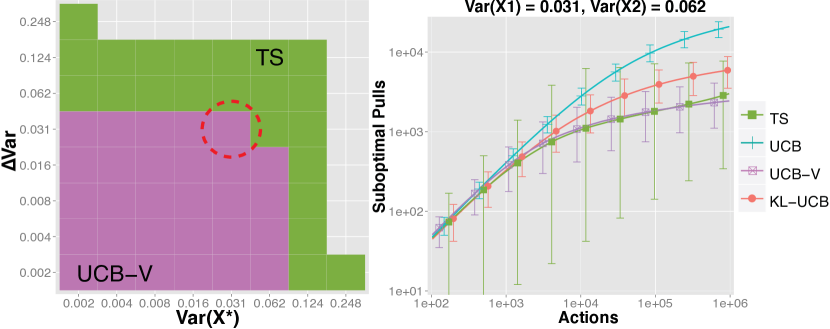
Figure 1: Left: Tile plot indicating which approach achieved lowest regret (averaged over 2000 independent runs) in the 2-estimator scaled-Bernoulli setting, at time $10^{6}$. X-axis is the variance of the optimal estimator, and Y-axis is the additional variance on the second estimator. Right: Log-plot illustrating the expected number of suboptimal selections for the highlighted case (dashed red circle). Error bars indicate 99% empirical percentiles.

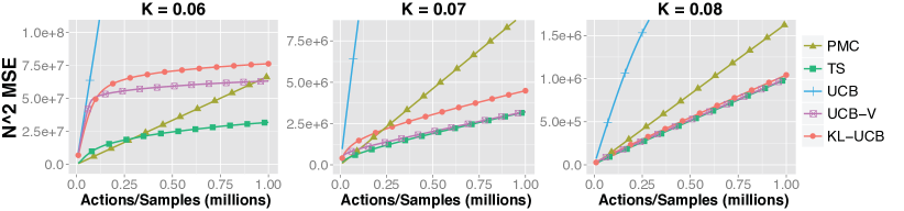
Figure 2: Plots showing the normalized MSE of different adaptive strategies for estimating the price of a European caplet option under the Cox-Ingersol-Ross interest rate model, using different strike prices (K). All results are statistically significant up to visual resolution.

In particular, we consider problems when $X_{k,t}=\mu+s_{k}(Z_{t}-\frac{1}{2})$, where $Z_{t}$ is standard Bernoulli and $s_{k}\!\in\!(0,1)$ is a separate scale parameter for $k\!\in\!\{1,2\}$. This design permits the maximum range for variance around a mean within a bounded interval. We evaluated the four bandit strategies detailed in Section 2: UCB1, UCB-V, KL-UCB, and TS, where for UCB-V we used the same settings as (Audibert et al., 2009), and for TS we used the uniform Beta prior, i.e., $\alpha_{0}=1$ and $\beta_{0}=1$.

The relative performance of these approaches is reported in Figure 1. TS appears best suited for scenarios where either estimator has high variance, whereas UCB-V is more effective when faced with medium or low variance estimators. Additionally, KL-UCB out-performs UCB-V in high variance settings, but in all such cases was eclipsed by TS.

6.2 Option Pricing

We next consider a more practical application of adaptive Monte Carlo estimation to the problem of pricing financial instruments. In particular, following (Douc et al., 2007; Arouna, 2004), we consider the problem of pricing European call options under the assumption that the interest rate evolves in time according to the Cox-Ingersoll-Ross (CIR) model (Cox et al., 1985), a popular model in mathematical finance (details provided in Appendix F). In a nutshell, this model assumes that the interest rate $r(t)$, as a function of time $t\!>\!0$, follows a square root diffusion model. The price of a European caplet option with “strike price” $K\!>\!0$, “nominee amount” $M\!>\!0$ and “maturity” $T\!>\!0$ is then given by $P=M\exp(-\int_{0}^{T}r(t)dt)\max(r(T)-K,0)$. The problem is to determine the expected value of $P$.

A naive approach to estimating $\mathbb{E}\left[P\right]$ is to simulate independent realizations of $r(t)$ for $0<t\leq T$. However, any simulation where the interest rate $r(T)$ lands below the strike price can be ignored since the payoff is zero. Therefore, a common estimation strategy is to use importance sampling by introducing a “drift” parameter $\theta>0$ into the proposal density for $r(t)$, with $\theta=0$ meaning no drift; this encourages simulations with higher interest rates. The importance weights for these simulations can then be efficiently calculated as a function of $\theta$ (see Appendix F).

Importantly, the task of adaptively allocating trials between different importance sampling estimators has been previously studied on this problem, using an unrelated technique known as d-kernel Population Monte Carlo (PMC) (Douc et al., 2007). Space restrictions prevent us from providing a full description of the PMC method, but, roughly speaking, the method defines the proposal density as mixture over the set $\{\theta_{k}\}$ of drift parameters considered. At each time step, PMC samples a new drift value according to this mixture and then simulates an interest rate. After a fixed number of samples, say $G$ (the population size), the mixture coefficient $\alpha_{k}$ of each drift parameter $\theta_{k}$ is adjusted by setting it to be proportional to the sum of importance weights sampled from that parameter: $\alpha_{k}=\frac{\sum_{t=1}^{G}w_{t}{\mathbb{I}\{{I_{t}=k}\}}}{\sum_{t=1}^{G}w_{t}}$. The new proposal is then used to generate the next population.

We approximated the option prices under the same parameter settings as (Douc et al., 2007), namely, $\nu=0.016$, $\kappa\!=\!0.2$, $r_{0}\!=\!0.08$, $T=1$, $M\!=\!1000$, $\sigma\!=\!0.02$, and $n\!=\!100$, for different strike prices $K\!=\!\{0.06,0.07,0.08\}$ (see Appendix F). However, we consider a wider set of proposals given by $\theta_{k}=k/10$ for $k\!\in\!\{0,1,...,15\}$. The results averaged over 1000 simulations are given in Figure 2.

These results generally indicate that the more effective bandit approaches are significantly better suited to this allocation task than the PMC approach, particularly in the longer term. Among the bandit based strategies, TS is the clear winner, which, given the conclusions from the previous experiment, is likely due to high level of variance introduced by the option pricing formula. Despite this strong showing for the bandit methods, PMC remains surprisingly competitive at this task, doing uniformly better than UCB, and better than all other bandit allocation strategies early on for $K=0.06$. However, we believe that this advantage of PMC stems from the fact that PMC explore the entire space of mixture distribution (rather than single $\theta_{k}$). It remains an interesting area for future work in bandit-based allocation strategies to extend the existing methods to continuously parameterized settings.

6.3 Adaptive Annealed Importance Sampling

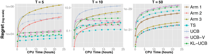
Figure 3: Plots showing the average regret (over 20 independent runs) of bandit allocators on the Logistic Regression model. $T$ is training sample size, “Arm 1/2/3” indicates each fixed estimator; and the one missing from a figure is the best for that setting. The solid lines indicate the performance of combining observations uniformly, whereas the dashed lines indicate the performance of combining observations using inverse variance weights.

Many important applications of Monte Carlo estimation occur in Bayesian inference, where a particularly challenging problem is evaluating the model evidence of a latent variable model. Evaluating such quantities is useful for a variety of purposes, such as Bayesian model comparison and testing/training set evaluation (Robert, 2012). However, the desired quantities are notoriously difficult to estimate in many important settings, due in no small part to the fact that popular high-dimensional Monte Carlo strategies, such as Markov Chain Monte Carlo (MCMC) methods, cannot be directly applied (Neal, 2005).

Nevertheless, a popular approach for approximating such values is annealed importance sampling (AIS) (Neal, 2001) (or more generally sequential Monte Carlo samplers (Del Moral et al., 2006)). In a nutshell, AIS combines the advantages of importance sampling with MCMC by defining a proposal density through a sequence of MCMC transitions applied to a sequence of annealed distributions, which slowly blend between the proposal (prior) and the target (un-normalized posterior). While such a technique can offer impressive practical advantages, it often requires considerable effort to set parameters; in particular, the practitioner must specify the number of annealing steps, the annealing rate or “schedule”, the underlying MCMC method (and its parameters), and the number of MCMC transitions to execute at annealing step. Even when these parameters have been appropriately tuned on preliminary data, there is no assurance that these choices will remain effective when deployed on larger or slightly different data sets.

Here we consider the problem of approximating the normalization constant for a Bayesian logistic regression model on different sized subsets of the 8-dimensional Pima Indian diabetes UCI data set (Bache & Lichman, 2013). We consider the problem of allocating resources between three AIS estimators that differ only in the number of annealing steps they use; namely, 400, 2000, and 8000 steps. In each case, we fix the annealing schedule using the power of 4 heuristic suggested by (Kuss & Rasmussen, 2005), with a single slice sampling MCMC transition used at each step (Neal, 2003) (this entails one “step” in each of the 8 dimensions); see Appendix G for further details.

A key challenge in this scenario is that the computational costs associated with each arm differ substantially, and, because slice sampling uses an internal rejection sampler, these costs are stochastic. To account for these costs we directly use elapsed CPU-time when drawing a sample from each estimator, as reported by the java vm. This choice reflects the true underlying cost and is particularly convenient since it does not require the practitioner to implement special accounting functionality. Since we do not expect this cost to correlate with the sample returns, we use the independent costs payoff formulation from Section 5: $-\tfrac{1}{4}(D_{k,2m}+D_{k,2m+1})(X_{k,2m}-X_{k,2m+1})^{2}$.

The results for the different allocation strategies for training sets of size 5, 10, and 50 are shown in Figure 3. Perhaps the most striking result is the performance improvement achieved by the nonuniformly combined estimators, which are indicated by the dashed lines. These estimators do not change the underlying allocation; instead they improve the final combined estimate by weighting each observation inversely proportional to the sample variance of the estimator that produced it. This performance improvement is an artifact of the nonuniform cost setting, since arms that are very close in terms of $V_{k}\delta_{k}$ can still have considerably different variances, which is especially true for AIS. Also observe that no one arm is optimal for all three training set sizes, consequently, we can see that bandit allocation (Thompson sampling in particular) is able to outperform any static strategy. In practice, this implies that even after exhaustive parameter tuning, automated adaptation can still offer considerable benefits simply due to changes in the data.

7 Conclusion

In this paper we have introduced a new sequential decision making strategy for competing with the best consistent Monte Carlo estimator in a finite pool. When each base estimator produces unbiased values at the same cost, we have shown that the sequential estimation problem maps to a corresponding bandit problem, allowing future improvements in bandit algorithms to be transfered to combining unbiased estimators. We have also shown a weaker reduction for problems where the different estimators take different (possibly random) time to produce an observation.

We expect this work to inspire further research in the area. For example, one may consider combining not only finitely many, but infinitely many estimators using appropriate bandit techniques (Bubeck et al., 2011), and/or exploit the fact that the observation from one estimator may reveal information about the variance of others. This is the case for example when the samplers use importance sampling, leading to the (new) stochastic variant of the problem known as “bandits with side-observations” (Mannor & Shamir, 2011; Alon et al., 2013). However, much work remains to be done, such studying in detail the use variance weighted estimators, dealing with continuous families of estimators, or a more thorough empirical investigation of the alternatives available.

Acknowledgements

This work was supported by the Alberta Innovates Technology Futures and NSERC. Part of this work was done while Cs.Sz. was visiting Technion, Haifa and Microsoft Research, Redmond, whose support and hospitality are greatly acknowledged.

Appendix A Proofs for Section 4

In this section we provide the proof of Theorem 1. For the proof, we will need the following two lemmas:

Lemma 1 (Optional Sampling).

Let $(X_{t})_{t\in\mathbb{N}}$ be a sequence of i.i.d. random variables, and $(X^{\prime}_{t})_{t\in\mathbb{N}}$ be its subsequence such that the decision whether to include $X_{t}$ in the subsequence is independent of future values in the sequence, i.e., $X_{s}$ for $s\geq t$. Then the sequence $(X^{\prime}_{t})_{t\in\mathbb{N}}$ is an i.i.d. sequence with the same distribution as $(X_{t})_{t\in\mathbb{N}}$.

Proof.

See Theorem 5.2 in Chapter III on page 145 of (Doob, 1953). ∎

We also need Wald’s second identity:

Lemma 2 (Wald’s Second Identity).

Let $(X_{t})_{t\in\mathbb{N}}$ be a sequence of $(\mathcal{F}_{t};t\geq 1)$-adapted random variables such that $\mathbb{E}\left[X_{t}|\mathcal{F}_{t-1}\right]=\mu$ and $\mathbb{E}\left[(X_{t}-\mu)^{2}|\mathcal{F}_{t-1}\right]=\sigma^{2}$ for any $t\geq 1$. Let $S_{n}=\sum_{t=1}^{n}X_{t}$ be the partial sum of the first $n$ random variables ($n\geq 1$) and $\tau>0$ be some stopping time w.r.t. $(\mathcal{F}_{t};t\geq 1)$. Then,

$$\mathbb{E}\left[(S_{\tau}-\mu\tau)^{2}\right]=\sigma^{2}\mathbb{E}\left[\tau\right]\,.$$

Proof.

See Theorem 14.3 of (Gut, 2005). ∎

Now, let us return to the proof of Theorem 1. Let $I_{t}\in\{1,\ldots,K\}$ denote the choice that $\mathcal{A}$ made at the beginning of round $t$ and recall that $T_{k}(t)=\sum_{s=1}^{t}{\mathbb{I}\{{I_{s}=k}\}}$. The observation at the end of round $t$ is $Y_{t}=X_{I_{t},T_{I_{t}}(t)}$ and the cumulative sum of returns after $n$ rounds for arm $k$ is $S_{k,n}=\sum_{t=1}^{T_{k}(n)}X_{k,t}$. Likewise, $S_{n}=\sum_{t=1}^{n}Y_{t}=\sum_{k=1}^{K}S_{k,n}$. By definition, the estimate after $n$ rounds is

$$\hat{\mu}_{n}=\frac{S_{n}}{n}=\frac{1}{n}\sum_{k=1}^{K}S_{k,n}\,.$$

Since the variance of this estimate does not depend on the mean, without loss of generality we may consider the case when $\mu=0$, giving

$$L_{n}(\mathcal{A}) =\mathbb{E}\left[\hat{\mu}_{n}^{2}\right]=\frac{1}{n^{2}}\mathbb{E}\left[\sum_{k=1}^{K}S_{k,n}^{2}+2\sum_{k\neq j}S_{k,n}S_{j,n}\right]$$ (11)

We may then observe that for any $k\neq j$,

$$\mathbb{E}\left[S_{k,n}S_{j,n}\right] =\mathbb{E}\left[({\mathbb{I}\{{I_{n}=k}\}}Y_{n}+S_{k,n-1})({\mathbb{I}\{{I_{n}=j}\}}Y_{n}+S_{j,n-1})\right]$$

$$=\mathbb{E}[\cancel{{\mathbb{I}\{{I_{n}=k}\}}{\mathbb{I}\{{I_{n}=j}\}}Y^{2}_{n}}+{\mathbb{I}\{{I_{n}=k}\}}Y_{n}S_{j,n-1}+{\mathbb{I}\{{I_{n}=j}\}}Y_{n}S_{k,n-1}+S_{k,n-1}S_{j,n-1}].$$

By considering the conditional expectation w.r.t. the history up to $Y_{n}$ (including $I_{n}$), i.e., w.r.t. $\mathcal{F}_{n-1}=\sigma(Y_{1},\ldots,Y_{n-1},I_{1},\ldots,I_{n})$, we have

$$\mathbb{E}[S_{k,n}S_{j,n}] =\mathbb{E}\left[\mathbb{E}\left[S_{k,n}S_{j,n}|\mathcal{F}_{n-1}\right]\right]$$

$$=\mathbb{E}[({\mathbb{I}\{{I_{n}=k}\}}S_{j,n-1}+{\mathbb{I}\{{I_{n}=j}\}}S_{k,n-1})\,\mathbb{E}[Y_{n}|\mathcal{F}_{n-1}]]+\mathbb{E}[S_{k,n-1}S_{j,n-1}].$$

Now, since $I_{n}\in\{1,\ldots,K\}$ and $I_{n}$ is $\mathcal{F}_{n-1}$]-measurable, $\mathbb{E}\left[Y_{n}|\mathcal{F}_{n-1}\right]=\sum_{k=1}^{K}{\mathbb{I}\{{I_{n}=k}\}}\mathbb{E}\left[X_{k,T_{k}(n)}|\mathcal{F}_{n-1},I_{n}=k\right]$. Further, by Lemma 1, $(X_{k,T_{k}(n)})_{n}$ is an i.i.d. sequence, sharing the same distribution as $(X_{k,t})_{t}$. Since $\sigma(X_{k,T_{k}(n)})$ is independent of $\sigma(Y_{1},\ldots,Y_{n-1},I_{1},\ldots,I_{n-1},I_{n},I_{n}=k)$, $\mathbb{E}\left[X_{k,T_{k}(n)}|\mathcal{F}_{n-1},I_{n}=k\right]=\mathbb{E}\left[X_{k,T_{k}(n)}\right]=\mu=0$. Therefore,

$$\mathbb{E}\left[S_{k,n}S_{j,n}\right]=\mathbb{E}[S_{k,n-1}S_{j,n-1}]=\ldots=\mathbb{E}[S_{k,0}S_{j,0}]=0.$$

As a result, (11) becomes

$$L_{n}(\mathcal{A})=\frac{1}{n^{2}}\mathbb{E}\left[\sum_{k=1}^{K}S_{k,n}^{2}\right]=\frac{1}{n^{2}}\sum_{k=1}^{K}\mathbb{E}[S_{k,n}^{2}].$$

From Wald’s second identity (cf. Lemma 2) we conclude $\mathbb{E}[S^{2}_{k,n}]=\mathbb{V}(X_{k})\mathbb{E}[T_{k}(n)]$ and thus get

$$L_{n}(\mathcal{A})=\frac{1}{n^{2}}\sum_{k=1}^{K}\mathbb{V}(X_{k})\mathbb{E}[T_{k}(n)].$$ (12)

Using the definition of the normalized MSE-regret and that $\min_{1\leq k\leq K}L_{k,n}=V^{*}/n$,

$$R_{n}(\mathcal{A})=n^{2}\left(L_{n}(\mathcal{A})-\frac{V^{*}}{n}\right)=\sum_{k=1}^{K}\mathbb{E}[T_{k}(n)](V_{k}-V^{*}),$$

which was the result to be proven.

Appendix B Handling Unknown Ranges

The algorithms and bounds of Section 4 can be easily extended to the setting where $X_{k,t}\in[a_{k},b_{k}]$ (often $a=0$) where $a_{k}<b_{k}$ are a priori known. One option is to scale $X_{k,t}$ to the common range $[0,1]$ using $\tilde{X}_{k,t}=(X_{k,t}-\min_{k}a_{k})/(\max_{k}b_{k}-\min_{k}a_{k})$ and then feed $1-\tilde{X}_{k,t}^{2}$ to the bandit algorithms (as the bandit algorithms expect the rewards in $[0,1]$ and constant translation of each reward does not change the regret). However, as these algorithms (prepared for “worst case” distributions) are sensitive to the overestimation of the range, this would lead to an unnecessary deterioration of the performance. A better option is to scale each variable separately. Then, the upper-confidence bound based algorithms must be modified by scaling each of the rewards with respect to its own range and then the bounds needs to be scaled back to the original range. Thus, the method that computes the reward upper bounds must be fed with $\frac{(b_{k}-a_{\min})^{2}-(X_{k,m}-a_{\min})^{2}}{(b_{k}-a_{\min})^{2}}\in[0,1]$, where $a_{\min}=\min_{1\leq k\leq K}a_{k}$. Then, if the method returns an upper bound $B_{k,m}$, the bound to be used for selecting the best arm (which should be an upper bound for $-\mathbb{E}\left[(X_{k,t}-a_{\min})^{2}\right]$) should be $B^{\prime}_{k,t}=(b_{k}-a_{\min})^{2}(B_{k,t}-1)$. Here we exploit that $-\mathbb{E}\left[(X_{k,t}-a_{\min})^{2}\right]=-\mathbb{E}\left[X_{k,t}^{2}\right]+c$ where the constant $c=2\mu a_{\min}-a_{\min}^{2}$ (which is neither known, nor needs to be known or estimated) is common to all the estimators, hence finding the arm that maximizes $-\mathbb{E}\left[(X_{k,t}-a_{\min})^{2}\right]$ is equivalent to finding the arm that maximizes $-\mathbb{E}\left[X_{k,t}^{2}\right]$. Since the confidence bounds will be loser if the range is larger, we thus see that the algorithm may be sensitive to the ranges $r_{k}=b_{k}-a_{\min}$. In particular, the $1/n$-term in the bound used by UCB-V will scale with $r_{k}^{2}$ and may dominate the bound for smaller values of $n$. In fact, UCB-V needs $n\approx r_{k}^{2}$ samples before this term becomes negligible, which means that for such estimators, the upper confidence bound of UCB-V will be above $1$ for $r_{k}^{2}$ steps. Even if we cut the upper confidence bounds at $1$, UCB-V will keep using these arms with a large range $r_{k}$ defending against the possibility that the sample variance crudely underestimates the true variance. Since the bound of KL-UCB is in the range $[0,1]$, KL-UCB is less exposed to this problem.

Based on Theorem 1, an alternative is to use bandit algorithms to minimize cost where the cost of an arm is defined as the variance of samples from that arm. This may be advantageous when the ranges become large because of unequal lower bounds $(a_{k})$. To implement this idea one needs to develop new bandit algorithms for cumulative variance minimization, which in fact is explored in Section 5, in the context of estimation under nonuniform-costs.

Finally, note that the assumption that the samples belong to a known bounded interval is not necessary (it was not used in the reduction results). In fact, the upper-confidence based bandit algorithms mentioned can also be applied when the payoffs are subgaussian with a known subgaussian coefficient, or even if the tail is heavier (Bubeck & Cesa-Bianchi, 2012a; Bubeck et al., 2013). In fact, the weaker assumptions under which the multi-armed bandit problem with finitely many arms has been analyzed assumes only that the $1+\varepsilon$ moment of the payoff is finite for some known $\varepsilon$ with a known moment bound (Bubeck et al., 2013). These strategies must replace the sample means with more robust estimators and also modify the way the upper confidence bounds are calculated. In our setting, the condition on the moment transfers to the assumption that the $2+\varepsilon$ moment $\mathbb{E}\left[|X_{k,t}|^{2+\varepsilon}\right]$ must be finite with a known upper bound for some $\varepsilon$.

Appendix C Proofs for Section 5

In this section we provide the proof of Theorem 5.

We can write the MSE at time $t$ as $L(\mathcal{A},t)=\mathbb{E}\left[\left(\frac{S(t)-(N(t)-1)\mu}{N(t)-1}\right)^{2}\right]$. The first step is to replace the denominator with its expectation. The price of this is calculated in the following result:

Lemma 3.

Let $S,N$ be random variables, $N\geq 0$ such that $\mathbb{E}\left[N\right]>0$, $\mu\in$. Let $D={\mathbb{I}\{{N=0}\}}(a-\mu)+{\mathbb{I}\{{N\neq 0}\}}\left(\frac{S}{N}-\mu\right)$. Let $d\in\mathbb{R}$ be an almost sure upper bound on $|D|{\mathbb{I}\{{N\neq 0}\}}$. Then, for any $c\geq 0$,

$$\mathbb{E}\left[D^{2}\right] \leq(a-\mu)^{2}\mathbb{P}(N=0)+\frac{\mathbb{E}\left[(S-N\mu)^{2}\right]}{\mathbb{E}\left[N\right]^{2}}\left(1+\frac{2c}{\sqrt{\mathbb{E}\left[N\right]}}\right)^{2}+d^{2}\left[\mathbb{P}(N<\mathbb{E}\left[N\right]-c\sqrt{\mathbb{E}\left[N\right]})+{\mathbb{I}\{{\mathbb{E}\left[N\right]<4c^{2}}\}}\right]\,.$$ (13)

Further, assuming that $S=0$ almost surely on $\{N=0\}$,

$$\mathbb{E}\left[D^{2}\right] \geq(a-\mu)^{2}\mathbb{P}(N=0)+\frac{\mathbb{E}\left[(S-N\mu)^{2}\right]}{\mathbb{E}\left[N\right]^{2}}\left(1-\frac{2c}{\sqrt{\mathbb{E}\left[N\right]}}\right)-d^{2}\,\frac{\mathbb{E}\left[N^{2}\right]}{\mathbb{E}\left[N\right]^{2}}\,\mathbb{P}(N>\mathbb{E}\left[N\right]+c\sqrt{\mathbb{E}\left[N\right]})\,.$$

The lemma is useful when $N$ concentrates around its mean. Consider the upper bound on $\mathbb{E}\left[D^{2}\right]$. In general, we expect $\mathbb{P}(N<\mathbb{E}\left[N\right]-C\sqrt{\mathbb{E}\left[N\right]\log(1/\delta)})\leq\delta$ with some numerical constant $C$. Thus, setting $c=C\sqrt{\log(1/\delta)}$ results in $d^{2}\left[\mathbb{P}(N<\mathbb{E}\left[N\right]-c\sqrt{\mathbb{E}\left[N\right]})+{\mathbb{I}\{{\mathbb{E}\left[N\right]<4c^{2}}\}}\right]\leq d^{2}\delta+d^{2}{\mathbb{I}\{{\mathbb{E}\left[N\right]<4C^{2}\log(1/\delta)}\}}$. Imagine now that $\mathbb{E}\left[N\right]=rt$ and choose $\delta=t^{-q}$ with $q>0$. Then, as soon as $rt>4C^{2}\sqrt{q\log(t)}$, the last indicator of (13) becomes zero. Further, $\frac{2c}{\sqrt{\mathbb{E}\left[N\right]}}=\sqrt{\frac{2q\log(t)}{rt}}\rightarrow 0$ as $t\rightarrow\infty$. Since this term converges at a $1/\sqrt{t}$ rate, we should choose $q\geq 1/2$, so that $\delta=\delta(t)$ converges at least as fast as this term. However, since later “$D$ gets multiplied by $t^{2}$”, to get a sublinear rate matching other terms, one should choose $q\geq 3/2$.

Proof.

Let $b=c\sqrt{\mathbb{E}\left[N\right]}$. First we prove the upper bound. We have

$$\mathbb{E}\left[D^{2}\right] \leq\mathbb{E}\left[D^{2}{\mathbb{I}\{{N=0}\}}\right]+\mathbb{E}\left[D^{2}{\mathbb{I}\{{N\neq 0,N\geq\mathbb{E}\left[N\right]-b,b\leq\tfrac{1}{2}\mathbb{E}\left[N\right]}\}}\right]+\mathbb{E}\left[D^{2}{\mathbb{I}\{{N\neq 0,N<\mathbb{E}\left[N\right]-b}\}}\right]$$

$$\qquad+\mathbb{E}\left[D^{2}{\mathbb{I}\{{N\neq 0,b>\tfrac{1}{2}\mathbb{E}\left[N\right]}\}}\right]$$

$$\leq(a-\mu)^{2}\mathbb{P}(N=0)+\mathbb{E}\left[\frac{(S-N\mu)^{2}}{(\mathbb{E}\left[N\right]-b)^{2}}{\mathbb{I}\{{b\leq\tfrac{1}{2}\mathbb{E}\left[N\right]}\}}\right]+d^{2}\mathbb{P}(N<\mathbb{E}\left[N\right]-b)+d^{2}{\mathbb{I}\{{b>\tfrac{1}{2}\mathbb{E}\left[N\right]}\}}$$

$$\leq(a-\mu)^{2}\mathbb{P}(N=0)+\frac{\mathbb{E}\left[(S-N\mu)^{2}\right]}{(\mathbb{E}\left[N\right]-b)^{2}}{\mathbb{I}\{{b\leq\tfrac{1}{2}\mathbb{E}\left[N\right]}\}}+d^{2}\mathbb{P}(N<\mathbb{E}\left[N\right]-b)+d^{2}{\mathbb{I}\{{b>\tfrac{1}{2}\mathbb{E}\left[N\right]}\}}\,.$$

Noting that $1/(1-x)\leq 1+2x$ when $0\leq x\leq 1/2$, we get that

$$\frac{1}{\mathbb{E}\left[N\right]-b}{\mathbb{I}\{{b\leq\tfrac{1}{2}\mathbb{E}\left[N\right]}\}}=\frac{1}{\mathbb{E}\left[N\right]}\,\frac{1}{1-\frac{b}{\mathbb{E}\left[N\right]}}{\mathbb{I}\{{b\leq\tfrac{1}{2}\mathbb{E}\left[N\right]}\}}\leq\frac{1}{\mathbb{E}\left[N\right]}\,\left(1+2\frac{b}{\mathbb{E}\left[N\right]}\right)=\frac{1}{\mathbb{E}\left[N\right]}\left(1+2\frac{c}{\sqrt{\mathbb{E}\left[N\right]}}\right)\,.$$

Putting things together, we get the desired upper bound.

The lower bound is proved in a similar fashion. To simplify notation, let $\mathcal{N}$ denote the event $\{0<N\leq\mathbb{E}\left[N\right]+b\}$. Then,

$$\mathbb{E}\left[D^{2}\right] \geq(a-\mu)^{2}\mathbb{P}(N=0)+\mathbb{E}\left[\left(\frac{(S-N\mu)}{N}\right)^{2}{\mathbb{I}\{{\mathcal{N}}\}}\right]$$

$$\geq(a-\mu)^{2}\mathbb{P}(N=0)+\mathbb{E}\left[\frac{(S-N\mu)^{2}}{(\mathbb{E}\left[N\right]+b)^{2}}{\mathbb{I}\{{\mathcal{N}}\}}\right]$$

$$=(a-\mu)^{2}\mathbb{P}(N=0)+\mathbb{E}\left[\frac{(S-N\mu)^{2}}{(\mathbb{E}\left[N\right]+b)^{2}}\right]-\mathbb{E}\left[\frac{(S-N\mu)^{2}}{(\mathbb{E}\left[N\right]+b)^{2}}{\mathbb{I}\{{N=0\text{ or }N>\mathbb{E}\left[N\right]+b}\}}\right]$$

$$\geq(a-\mu)^{2}\mathbb{P}(N=0)+\frac{\mathbb{E}\left[N\right]^{2}}{(\mathbb{E}\left[N\right]+b)^{2}}\frac{\mathbb{E}\left[(S-N\mu)^{2}\right]}{\mathbb{E}\left[N\right]^{2}}-\mathbb{E}\left[\frac{(S-N\mu)^{2}}{(\mathbb{E}\left[N\right]+b)^{2}}{\mathbb{I}\{{N>\mathbb{E}\left[N\right]+b}\}}\right]$$

$$\qquad\qquad(\text{because by assumption }\mathbb{E}\left[(S-N\mu)^{2}{\mathbb{I}\{{N=0}\}}\right]=0)$$

$$=(a-\mu)^{2}\mathbb{P}(N=0)+\frac{\mathbb{E}\left[N\right]^{2}}{(\mathbb{E}\left[N\right]+b)^{2}}\frac{\mathbb{E}\left[(S-N\mu)^{2}\right]}{\mathbb{E}\left[N\right]^{2}}-\frac{\mathbb{E}\left[N^{2}\right]}{(\mathbb{E}\left[N\right]+b)^{2}}\left(d^{2}\mathbb{P}(N>\mathbb{E}\left[N\right]+b)\right)$$

$$\geq(a-\mu)^{2}\mathbb{P}(N=0)+\left(1-\frac{2b}{\mathbb{E}\left[N\right]}\right)\frac{\mathbb{E}\left[(S-N\mu)^{2}\right]}{\mathbb{E}\left[N\right]^{2}}-d^{2}\,\frac{\mathbb{E}\left[N^{2}\right]\,\mathbb{P}(N>\mathbb{E}\left[N\right]+b)}{\mathbb{E}\left[N\right]^{2}}\,,$$

where in the last inequality we used

$$\frac{\mathbb{E}\left[N\right]^{2}}{(\mathbb{E}\left[N\right]+b)^{2}}=\left(1-\frac{b}{\mathbb{E}\left[N\right]+b}\right)^{2}\geq 1-\frac{2b}{\mathbb{E}\left[N\right]+b}$$

and $1/(\mathbb{E}\left[N\right]+b)\leq 1/\mathbb{E}\left[N\right]$. ∎

The above lemma suggests that when bounding $\mathbb{E}\left[(S/N-\mu)^{2}\right]$, the main term is $\mathbb{E}\left[(S-N\mu)^{2}\right]/\mathbb{E}\left[N\right]^{2}$. First we develop a lower bound on this when only sampler $k$ is used at every time step.

Lemma 4.

Let Assumption 5.1 hold and assume that the random variables $|X_{k,m}-\mu|_{k,m}$ are a.s. bounded by some constant $B>0$. Consider the case when an individual sampler $k\in\{1,\ldots,K\}$ is used up to time $t$: Let $N_{k}(t)$ be the smallest integer such that $\sum_{m=1}^{N_{k}(t)}D_{k,m}\geq t$ and $S_{k}(t)=\sum_{m=1}^{N_{k}(t)-1}X_{k,m}$. Then, for any $t>0$ such that $\mathbb{E}\left[N_{k}(t)\right]>1$, and for any constant $\beta>0$ such that $\mathbb{P}(D_{k,1}\leq\beta)>0$,

$$\frac{\mathbb{E}\left[(S_{k}(t)-(N_{k}(t)-1)\mu)^{2}\right]}{\mathbb{E}\left[N_{k}(t)-1\right]^{2}}\geq\frac{\delta_{k}V_{k}}{t+\beta}-2B\frac{\delta_{k}\sqrt{V_{k}\delta_{k}}}{t^{3/2}}-\frac{V_{k}\mathbb{E}\left[D_{k,1}{\mathbb{I}\{{D_{k,1}>\beta}\}}\right]}{t}\,$$ (14)

and

$$\frac{t}{\delta_{k}}\leq\mathbb{E}\left[N_{k}(t)\right]\leq\frac{t+\beta}{\delta_{k}-\mathbb{E}\left[D_{k,1}{\mathbb{I}\{{D_{k,1}>\beta}\}}\right]},$$ (15)

If the random variables $(D_{k,m})$ are a.s. bounded by a constant, we can choose $\beta$ to be their common upper bound to cancel the third term of (14). Otherwise, we need to select $\beta$ to strike a good balance between the first and third terms. Note that $\beta=o(t)$ makes the first the same order as $\delta_{k}V_{k}/t$ with an error term of order $\beta/t^{2}$. Thus, a reasonable choice is $\beta=t^{3/2}$, which makes the error term of the same order as the second term of the lower bound.

Proof.

We start with the proving the upper bound on $\mathbb{E}\left[N_{k}(t)\right]$ in (15). Define $\hat{D}_{k,m}=\min\{D_{k,m},\beta\}$ and let $\hat{N}_{k}(t)$ be the smallest integer such that $\sum_{m=1}^{\hat{N}_{k}(t)}\hat{D}_{k,m}\geq t$. Then, clearly $\hat{N}_{k}(t)\geq N_{k}(t)$, and by Wald’s identity,

$$t >\mathbb{E}\left[\sum_{m=1}^{\hat{N}_{k}(t)-1}\hat{D}_{k,m}\right]\geq\mathbb{E}\left[\sum_{m=1}^{\hat{N}_{k}(t)}\hat{D}_{k,m}\right]-\beta$$

$$=\mathbb{E}\left[\hat{N}_{k}(t)\right]\mathbb{E}\left[\hat{D}_{k,1}\right]-\beta\geq\mathbb{E}\left[N_{k}(t)\right](\delta_{k}-\mathbb{E}\left[D_{k,1}{\mathbb{I}\{{D_{k,1}>\beta}\}}\right])-\beta.$$

Therefore,

$$\mathbb{E}\left[N_{k}(t)\right]\leq\frac{t+\beta}{\delta_{k}-\mathbb{E}\left[D_{k,1}{\mathbb{I}\{{D_{k,1}>\beta}\}}\right]},$$

where we used that $\delta_{k}-\mathbb{E}\left[D_{k,1}{\mathbb{I}\{{D_{k,1}>\beta}\}}\right]>0$, which follows from our assumption $\mathbb{P}(D_{k,1}\leq\beta)>0$, finishing the proof of the upper bound. As for the lower bound, by the definition of $N_{k}(t)$ and Wald’s identity we have $\mathbb{E}\left[N_{k}(t)\right]\delta_{k}\geq t$, thus finishing the proof of (15).

Let us now turn to proving (14). We would like to apply Wald’s second identity to $(S_{k}(t)-(N_{k}(t)-1)\mu)^{2}$. However, while $N_{k}(t)$ is a stopping time w.r.t. the (natural) filtration $\mathcal{F}_{m}=\sigma(X_{k,1},D_{k,1},\ldots,X_{k,m},D_{k,m})$, $N_{k}(t)-1$ is not. Define $F=\sum_{m=1}^{N_{k}(t)}X_{k,m}-N_{k}(t)\mu$: We can apply Wald’s identity to $F$. Since $(S_{k}(t)-(N_{k}(t)-1)\mu)^{2}=F-(X_{k,N_{k}(t)}-\mu)$ we get

$$\mathbb{E}\left[(S_{k}(t)-(N_{k}(t)-1)\mu)^{2}\right] =\mathbb{E}\left[F^{2}\right]+\mathbb{E}\left[(X_{k,N_{k}(t)}-\mu)^{2}\right]-2\mathbb{E}\left[(X_{k,N_{k}(t)}-\mu)F\right]$$

$$\geq\mathbb{E}\left[N_{k}(t)\right]V_{k}-2\mathbb{E}\left[(X_{k,N_{k}(t)}-\mu)F\right]$$

$$\geq\mathbb{E}\left[N_{k}(t)\right]V_{k}-2B(\mathbb{E}\left[F^{2}\right])^{1/2}$$

$$=\mathbb{E}\left[N_{k}(t)\right]V_{k}-2B\sqrt{\mathbb{E}\left[N_{k}(t)\right]V_{k}}\,,$$ (16)

where in the second and last equality we used Lemma 2.

Combining (15) with (16), we obtain

$$\frac{\mathbb{E}\left[(S_{k}(t)-(N_{k}(t)-1)\mu)^{2}\right]}{\mathbb{E}\left[N_{k}(t)-1\right]^{2}} \geq\frac{\mathbb{E}\left[N_{k}(t)\right]V_{k}}{\mathbb{E}\left[N_{k}(t)\right]^{2}}-\frac{2B\sqrt{\mathbb{E}\left[N_{k}(t)\right]V_{k}}}{\mathbb{E}\left[N_{k}(t)\right]^{2}}$$

$$=\frac{V_{k}}{\mathbb{E}\left[N_{k}(t)\right]}-\frac{2B\sqrt{\mathbb{E}\left[N_{k}(t)\right]V_{k}}}{\mathbb{E}\left[N_{k}(t)\right]^{2}}$$

$$\geq\frac{\delta_{k}V_{k}}{t+\beta}-\frac{V_{k}\mathbb{E}\left[D_{k,1}{\mathbb{I}\{{D_{k,1}>\beta}\}}\right]}{t+\beta}-\frac{2B\sqrt{\mathbb{E}\left[N_{k}(t)\right]V_{k}}}{\mathbb{E}\left[N_{k}(t)\right]^{2}}$$

$$\geq\frac{\delta_{k}V_{k}}{t+\beta}-\frac{V_{k}\mathbb{E}\left[D_{k,1}{\mathbb{I}\{{D_{k,1}>\beta}\}}\right]}{t+\beta}-2B\frac{\delta_{k}\sqrt{V_{k}\delta_{k}}}{t^{3/2}}\,.$$

∎

In the next result we give an upper bound on $\mathbb{E}\left[(S(t)-(N(t)-1)\mu)^{2}\right]/\mathbb{E}\left[N(t)-1\right]^{2}$. Before stating this lemma, let us recall the definitions of $(I_{m})_{m=1,2,\ldots}$, $(T_{k}(m))_{m=0,1,\ldots,1\leq k\leq K}$, $(Y_{m})_{m=1,2,\ldots}$, $(J_{m})_{m=0,1,2,\ldots}$ and $(N(t))_{t\geq 0}$: $I_{m}\in\{1,\ldots,K\}$ is the index of the sampler chosen by $\mathcal{A}$ for round $m$; $T_{k}(m)=\sum_{s=1}^{m}{\mathbb{I}\{{I_{s}=k}\}}$ is the number of samples obtained from sampler $k$ by the end of round $m$ (the empty sum is defined as zero); $Y_{m}=X_{I_{m},T_{I_{m}}(m)}$ is the $m$th sample observed by $\mathcal{A}$; $J_{0}=0$ and $J_{m+1}=\sum_{s=1}^{m}D_{I_{s},T_{I_{s}}(s)}$ is the time when $\mathcal{A}$ observes the $(m+1)$th sample, and so the $m$th round lasts over the time period $[J_{m},J_{m+1})$; and $N(t)=\min\left\{m\,:\,J_{m}\geq t\right\}$ is the index of the round at time $t$ (the indexing of rounds starts at one). Thus, $N(t)-1$ is the number of samples observed over the time period $[0,t]$. Note that $\sum_{k=1}^{K}T_{k}(m)=m$ for any $m\geq 0$ and thus, in particular, $\sum_{k=1}^{K}T_{k}(N(t))=N(t)$. Further, remember that $S_{m}=\sum_{s=1}^{m}Y_{m}$ and $S(t)=S_{N(t)-1}$.

Lemma 5.

Let Assumption 5.1 hold and assume that the random variables $|X_{k,m}-\mu|_{k,m}$ are a.s. bounded by some constant $B>0$ and that $k^{*}={\arg\min}_{1\leq k\leq K}\delta_{k}V_{k}$ is unique. For $s\geq 0$, let $f(s)=\max_{k\neq k^{*}}\mathbb{E}\left[T_{k}(N(s)-1)\right]$ and assume that $c_{f}=\sup_{s>0}f(s)/s<+\infty$. Suppose that $t\geq 2\delta_{\max}$ and $\mathbb{E}\left[N(t)-1\right]>1$. Then,

$$\frac{\mathbb{E}\left[(S(t)-(N(t)-1)\mu)^{2}\right]}{\mathbb{E}\left[N(t)-1\right]^{2}} \leq\frac{\delta^{*}V^{*}}{t}+\frac{C}{t^{3/2}}+\frac{C^{\prime}f(t)}{t^{2}}$$ (17)

for some constants $C,C^{\prime}>0$ that depend only on the problem parameters $\delta_{k},V_{k}$ and $c_{f}$. Furthermore,

$$\mathbb{E}\left[N(t)-1\right]\geq\frac{t}{\delta_{\max}}-1\,.$$ (18)

Proof.

We proceed similarly to the proof of Lemma 4.

We first prove (18). By the definition of $N(t)$ and since $D_{k,m}$ is nonnegative for all $k$ and $m$,

$$t\leq J_{N(t)}\leq\sum_{s=1}^{N(t)}D_{I_{s},T_{I_{s}}(s)}=\sum_{k=1}^{K}\sum_{m=1}^{T_{k}(N(t))}D_{k,m}\,.$$

Notice that $(N(t))_{t\geq 0}$, $(T_{k}(n))_{n=0,1,\ldots}$ are stopping times w.r.t. the filtration $(\mathcal{F}_{m};m\geq 1)$, where $\mathcal{F}_{m}=\sigma(I_{1},J_{1},\ldots,I_{m},Y_{m})$. Therefore, $T_{k}(N(t))$ is also a stopping time w.r.t. $(\mathcal{F}_{m})$. Defining $\overline{T}_{k}(t)=\mathbb{E}\left[T_{k}(N(t))\right]$, Wald’s identity yields

$$t\leq\sum_{k=1}^{K}\mathbb{E}\left[T_{k}(N(t))\right]\delta_{k}=\sum_{k=1}^{K}\overline{T}_{k}(t)\delta_{k}\,.$$ (19)

Then,

$$\mathbb{E}\left[N(t)\right]=\sum_{k=1}^{K}\overline{T}_{k}(t)\geq\frac{1}{\delta_{\max}}\sum_{k=1}^{K}\overline{T}_{k}(t)\delta_{k}\geq\frac{t}{\delta_{\max}}\,,$$

finishing the proof of (18).

Now, let us turn to showing that (17) holds. First, notice that

$$S(t)-(N(t)-1)\mu =-(Y_{N(t)}-\mu)+\left\{S_{N(t)}-N(t)\mu\right\}=-(Y_{N(t)}-\mu)+\sum_{k=1}^{K}S_{k,T_{k}(N(t))}-T_{k}(N(t))\mu.$$

Hence, with the same calculation as in the proof of Theorem 1 (the difference is that here $N(t)$ is a stopping time while $n$ is a constant in Theorem 1), we get

$$\mathbb{E}\left[\sum_{k=1}^{K}\left\{S_{k,T_{k}(N(t))}-T_{k}(N(t))\mu\right\}^{2}\right]=\sum_{k=1}^{K}\overline{T}_{k}(t)V_{k}$$

and thus, introducing $F=S_{N(t)}-N(t)\mu$, $V_{\max}=\max_{k}V_{k}$, and $\bar{V}=\sum_{k\neq k^{*}}V_{k}$,

$$\mathbb{E}\left[(S(t)-(N(t)-1)\mu)^{2}\right] =-2\mathbb{E}\left[(Y_{N(t)}-\mu)F\right]+\mathbb{E}\left[(Y_{N(t)}-\mu)^{2}\right]+\sum_{k=1}^{K}\overline{T}_{k}(t)V_{k}$$

$$\leq 2B(\mathbb{E}\left[F^{2}\right])^{1/2}+V_{\max}+\sum_{k=1}^{K}\overline{T}_{k}(t)V_{k}$$

$$\leq 2B\sqrt{\sum_{k=1}^{K}\overline{T}_{k}(t)V_{k}}+V_{\max}+\sum_{k=1}^{K}\overline{T}_{k}(t)V_{k}$$ (20)

$$\leq 2B\sqrt{V_{\max}\sum_{k=1}^{K}\overline{T}_{k}(t)}+V_{\max}+\sum_{k=1}^{K}\overline{T}_{k}(t)V_{k}$$ (21)

$$=2B\sqrt{V_{\max}\mathbb{E}\left[N(t)\right]}+V_{\max}+\sum_{k=1}^{K}\overline{T}_{k}(t)V_{k}\,.$$ (22)

Introduce the notation $\bar{\delta}=\sum_{k\neq k^{*}}\delta_{k}$ and recall that, by assumption, $\overline{T}_{k}(t)\leq f(t)$ for all $k\neq k^{*}$. On the other hand, $\overline{T}_{k^{*}}(t)\leq\mathbb{E}\left[N(t)\right]$ holds trivially. Therefore, using (22), (19), and (18), we obtain

$$\frac{\mathbb{E}\left[(S(t)-(N(t)-1)\mu)^{2}\right]}{\mathbb{E}\left[N(t)-1\right]^{2}} \leq\frac{\left(\sum_{k=1}\overline{T}_{k}(t)\delta_{k}\right)\cdot\left\{\sum_{k=1}^{K}\overline{T}_{k}(t)V_{k}+2B\sqrt{V_{\max}\mathbb{E}\left[N(t)\right]}+V_{\max}\right\}}{t\,\mathbb{E}\left[N(t)-1\right]^{2}}$$

$$\leq\frac{\left(\overline{T}_{k^{*}}(t)\delta^{*}+f(t)\bar{\delta}\right)\left\{\overline{T}_{k^{*}}V_{k^{*}}+f(t)\bar{V}+2B\sqrt{V_{\max}\mathbb{E}\left[N(t)-1\right]+1}+V_{\max}\right\}}{t\,\mathbb{E}\left[N(t)-1\right]^{2}}$$

$$\leq\frac{\left(\mathbb{E}\left[N(t)-1\right]\delta^{*}+\delta^{*}+f(t)\bar{\delta}\right)\left\{\mathbb{E}\left[N(t)-1\right]V_{k^{*}}+f(t)\bar{V}+2B\sqrt{V_{\max}\mathbb{E}\left[N(t)-1\right]}+C_{0}\right\}}{t\,\mathbb{E}\left[N(t)-1\right]^{2}}$$

$$\leq\frac{\delta^{*}V^{*}}{t}+\frac{C_{1}}{t\,\sqrt{\mathbb{E}\left[N(t)-1\right]}}+\frac{C_{2}f(t)+C_{3}}{t\,\mathbb{E}\left[N(t)-1\right]}+\frac{C_{4}f^{2}(t)+C_{5}f(t)+C_{6}}{t\,\mathbb{E}\left[N(t)-1\right]^{2}}$$

$$\leq\frac{\delta^{*}V^{*}}{t}+\frac{\delta_{\max}^{1/2}C_{1}}{t\sqrt{t-\delta_{\max}}}+\frac{\delta_{\max}(C_{2}f(t)+C_{3})}{t(t-\delta_{\max})}+\frac{\delta_{\max}^{2}(C_{4}f^{2}(t)+C_{5}f(t)+C_{6})}{t(t-\delta_{\max})^{2}}$$

$$\leq\frac{\delta^{*}V^{*}}{t}+\frac{C}{t^{3/2}}+\frac{C^{\prime\prime}f(t)}{t^{2}}+\frac{C^{\prime\prime\prime}f^{2}(t)}{t^{3}}$$

$$\leq\frac{\delta^{*}V^{*}}{t}+\frac{C}{t^{3/2}}+\frac{C^{\prime}f(t)}{t^{2}}$$

where $C_{0},C_{1},C_{2},C_{3},C_{4},C_{5},C_{6},C,C^{\prime},C^{\prime\prime},C^{\prime\prime\prime}>0$ are appropriate constants depending on the problem parameters and $c_{f}$, and in the first to last step we used $t\geq 2\delta_{\max}$ and $f(t)\leq c_{f}t$ in the last step. This finishes the proof of the second part of the lemma. ∎

Combining the above two lemmas the proof of Theorem 5 is straightforward. We apply the first inequality of Lemma 3 to $\hat{D}=\hat{\mu}(t)-\mu=S(t)/(N(t)-1)-\mu$ and the second inequality of the lemma to $\hat{D}^{*}=\hat{\mu}_{k^{*}}(t)-\mu=S_{k}(t)/(N_{k^{*}}(t)-1)-\mu$. It is easy to see that $\mathbb{P}(N(t)=1)$ and $\mathbb{P}(N_{k^{*}}(t)=1)$ both decay exponentially fast, so the difference of the first terms is negligible. The difference of the second terms can be handled by Lemmas 4 and 5 and the bounds (15), (18) on $\mathbb{E}\left[N_{k^{*}}(t)\right]$, $\mathbb{E}\left[N(t)-1\right]$ (note that the lower bound on $\mathbb{E}\left[N(t)-1\right]$ can be simplified to $t/(2\delta_{\max})$ using $t\geq 2\delta_{\max}$): introducing $\lambda^{*}(\beta)=\mathbb{E}\left[D_{k^{*},1}{\mathbb{I}\{{D_{k^{*},1}>\beta}\}}\right]$ we obtain

$$\frac{\mathbb{E}\left[(S(t)-(N(t)-1)\mu)^{2}\right]}{\mathbb{E}\left[N(t)-1\right]^{2}}\left(1+\frac{2c}{\sqrt{\mathbb{E}\left[N(t)-1\right]}}\right)^{2}-\frac{\mathbb{E}\left[(S_{k^{*}}(t)-(N_{k^{*}}(t)-1)\mu)^{2}\right]}{\mathbb{E}\left[N_{k^{*}}(t)-1\right]^{2}}\left(1-\frac{2c}{\sqrt{\mathbb{E}\left[N_{k^{*}}(t)-1\right]}}\right)$$

$$\leq\left(\frac{\delta^{*}V^{*}}{t}+\frac{C}{t^{3/2}}+\frac{C^{\prime}f(t)}{t^{2}}\right)\left(1+\frac{2c\sqrt{2\delta_{\max}}}{\sqrt{t}}\right)^{2}-\left(\frac{\delta^{*}V^{*}}{t+\beta}-2B\frac{\delta^{*}\sqrt{\delta^{*}V^{*}}}{t^{3/2}}-\frac{V^{*}\lambda^{*}(\beta)}{t}\right)\,\left(1-\frac{c\sqrt{2\delta^{*}}}{\sqrt{t}}\right)$$

$$=\left(\frac{\delta^{*}V^{*}}{t}+\frac{C}{t^{3/2}}+\frac{C^{\prime}f(t)}{t^{2}}\right)\left(1+\frac{2c\sqrt{2\delta_{\max}}}{\sqrt{t}}+\frac{8c^{2}\delta_{\max}}{t}\right)-\left(\frac{\delta^{*}V^{*}}{t+\beta}-2B\frac{\delta^{*}\sqrt{\delta^{*}V^{*}}}{t^{3/2}}-\frac{V^{*}\lambda^{*}(\beta)}{t}\right)\,\left(1-\frac{c\sqrt{2\delta^{*}}}{\sqrt{t}}\right)$$

$$\leq\frac{\beta\,\delta^{*}V^{*}}{t(t+\beta)}+(c+C^{\prime\prime})t^{-3/2}+C^{\prime\prime\prime}f(t)t^{-2}+C^{\prime\prime\prime\prime}\lambda^{*}(\beta)t^{-1}$$

$$\leq\delta^{*}V^{*}\,\beta t^{-2}+(c+C^{\prime\prime})t^{-3/2}+C^{\prime\prime\prime}f(t)t^{-2}+C^{\prime\prime\prime\prime}\lambda^{*}(\beta)t^{-1}\,,$$

where we used that by assumption $c<\sqrt{t/(2\delta^{*})}$. Using $\mathbb{E}\left[N_{k^{*}}(t)-1\right]\geq t/(2\delta^{*})$, the last term in the bound of Lemma 3 for $\mathbb{E}\left[(\hat{\mu}_{k^{*}}(t)-\mu)^{2}\right]$ becomes $C_{1}t^{-2}\mathbb{E}\left[N_{k^{*}}(t)^{2}\right]\mathbb{P}(N_{k^{*}}(t)>\mathbb{E}\left[N_{k^{*}}(t)\right]+c\sqrt{\mathbb{E}\left[N_{k^{*}}(t)-1\right]})$. By $\mathbb{E}\left[N(t)-1\right]\geq t/(2\delta_{\max})$, the indicator in the third line of the bound for $\mathbb{E}\left[(\hat{\mu}(t)-\mu)^{2}\right]$ can be bounded as ${\mathbb{I}\{{\mathbb{E}\left[N(t)-1\right]<4c^{2}}\}}\leq{\mathbb{I}\{{t<8\delta_{\max}c^{2}}\}}$ which is zero since by assumption $c<\sqrt{t/(8\delta_{max})}$. Summing up our bounds and keeping the probability terms gives

$$\mathbb{E}\left[(\hat{\mu}(t)-\mu)^{2}\right]-\mathbb{E}\left[(\hat{\mu}_{k^{*}}(t)-\mu)^{2}\right] \leq\mu^{2}\left\{\mathbb{P}(N(t)=1)-\mathbb{P}(N_{k^{*}}(t)=1)\right\}$$

$$\qquad+\delta^{*}V^{*}\,\beta t^{-2}+(c+C^{\prime\prime})t^{-3/2}+C^{\prime\prime\prime}f(t)t^{-2}+C^{\prime\prime\prime\prime}\lambda^{*}(\beta)t^{-1}$$

$$\qquad+C_{1}t^{-2}\mathbb{E}\left[N_{k^{*}}(t)^{2}\right]\mathbb{P}(N_{k^{*}}(t)>\mathbb{E}\left[N_{k^{*}}(t)\right]+c\sqrt{\mathbb{E}\left[N_{k^{*}}(t)-1\right]})$$

$$\qquad+C_{2}\mathbb{P}(N(t)<\mathbb{E}\left[N(t)\right]-c\sqrt{\mathbb{E}\left[N(t)-1\right]})\,,$$

thus, finishing the proof.

Appendix D KL-Based Confidence Bound on Variance

The following lemma gives a variance estimate based on Kullback-Leibler divergence.

Lemma 6.

Let $Y_{1},\ldots,Y_{2n}$ and $Q_{1},\ldots,Q_{n}$ be two independent sequences of independent and identically distributed random variables taking values in $[0,1]$. Furthermore, for any $t=1,\ldots,n$, let

$$\bar{\mathbb{V}}_{2t}=\frac{1}{2t}\sum_{s=1}^{t}Q_{t}(Y_{2s}-Y_{2s-1})^{2}.$$ (23)

Then, for any $\delta>0$,

$$\mathbb{P}\left[\cup_{t=1}^{n}\left\{\operatorname{KL}\left(2\bar{\mathbb{V}}_{2t},2\mathbb{E}\left[Q_{1}\right]\mathbb{V}[Y_{1}]\right)\geq\frac{\delta}{t}\right\}\right]\leq 2e\lceil\delta\log n\rceil e^{-\delta}~{}.$$

Proof.

Equation (5) of Garivier (2013) states that if $Z_{1},\ldots,Z_{n}$ are independent, identically distributed random variables taking values in $[0,1]$ and $\bar{Z}_{t}=\frac{1}{t}\sum_{s=1}^{t}Z_{s}$ for $t=1,\ldots,n$, then for any $\delta>0$,

$$\mathbb{P}\left[\cup_{t=1}^{n}\left\{\operatorname{KL}\left(\bar{Z}_{t},\mathbb{E}\left[Z_{1}\right]\right)\geq\frac{\delta}{t}\right\}\right]\leq 2e\lceil\delta\log n\rceil e^{-\delta}~{}.$$

Defining $Z_{t}=Q_{t}(Y_{2t}-Y_{2t-1})^{2}$, we see that the above conditions on $Z_{t}$ are satisfied since they are clearly independent and identically distributed for $t=1,\ldots,n$, and $Z_{t}\in[0,1]$ since $0\leq Q_{t},Y_{2t-1},Y_{2t}\leq 1$. Now the statement of the lemma follows since $\mathbb{E}\left[Z_{t}\right]=\mathbb{E}\left[Q_{t}(Y_{2t}-Y_{2t-1})^{2}\right]=\mathbb{E}\left[Q_{t}\right]\mathbb{E}\left[((Y_{2t}-\mathbb{E}\left[Y_{2t}\right])-(Y_{2t-1}-\mathbb{E}{Y_{2t-1}}))^{2}\right]=2\mathbb{E}\left[Q_{1}\right]\mathbb{V}[Y_{1}]$. ∎

Corollary 1.

Let $Y_{1},\ldots,Y_{2n}$ and $Q_{1},\ldots,Q_{n}$ be two independent sequences of independent and identically distributed random variables taking values in $[0,1]$. For any $t=2,\ldots,n$, let $\bar{\mathbb{V}}_{t}$ be defined by (23) if $t$ is even, and let $\bar{\mathbb{V}}_{t}=\bar{\mathbb{V}}_{t-1}$ if $t$ is odd. Furthermore, let

$$\bar{\mathbb{V}}_{t,min}=\inf\{\mu:\operatorname{KL}\left(2\bar{\mathbb{V}}_{t},2\mu\right)\leq\delta/\lfloor t/2\rfloor\}$$

and

$$\bar{\mathbb{V}}_{t,max}=\sup\{\mu:\operatorname{KL}\left(2\bar{\mathbb{V}}_{t},2\mu\right)\leq\delta/\lfloor t/2\rfloor\}.$$

Then for any $\delta>0$, with probability at least $1-2e\lceil\delta\log\lfloor n/2\rfloor\rceil e^{-\delta}$,

$$\max_{2\leq t\leq n}\bar{\mathbb{V}}_{t,min}\leq\mathbb{E}\left[Q\right]\mathbb{V}[Y]\leq\min_{2\leq t\leq n}\bar{\mathbb{V}}_{t,max}\,.$$

Appendix E Details on Synthetic Experiments

In considering alternative bounded payout distributions we evaluated 3 natural choices, truncated normal, uniform, and scaled-Bernoulli. The latter non-standard distribution is a transformation of a Bernoulli described by three parameters, a midpoint $m\in\mathbb{R}$, a scale $s\in\mathbb{R}^{+}$, as well as a Bernoulli parameter $p$. Specifically, if $X\in\{0,1\}$ is a Bernoulli random variable with parameter $p$ then the transformation $m+(X-0.5)s$ provides the corresponding scaled-Bernoulli sample. We conducted experiments using these different distributions, keeping their variances the same, in an attempt to ascertain whether the shape of the distribution might affect the performance of the various bandit allocation algorithms. However, we were unable to uncover an instance where the shape of the distribution had a non-negligible effect on performance. As a result, we decided to conduct our experiments using scaled-Bernoulli distributions as they permit the maximum range for the variance in an bounded interval.

Appendix F The Cox-Ingersoll-Ross Model

In the Cox-Ingersoll-Ross (CIR) model the interest rate at time $t$, denoted $r(t)$, follows a square-root diffusion given by a stochastic differential equation of the form

$$dr(t)=(\eta-\kappa r(t))dt+\sigma\sqrt{r(t)}dW(t),$$

where $\eta$, $\kappa$ and $\sigma$ are fixed, problem-specific, constants and $W$ is a standard one-dimensional Brownian motion. The payoff of an option for this rate at time $T$ (maturity) is given as

$$M\max(r(T)-K,0),$$

where the strike price $K$ and nominee amount $M$ are parameters of the option. The actual quantify of interest, the price of an option at time $0$, is given as

$$\bar{P}\doteq\mathbb{E}\left[\exp(-\int_{0}^{T}r(t)dt)M\max(r(T)-K,0)\right].$$

The above integrals may approximated with the Monte Carlo method by first discretizing the interest rate trajectory, $r(t)$, into $n$ points $r_{1:n}$ and simulating

$$r_{t}=r_{t-1}+(\eta-\kappa r_{t-1})\frac{T}{n}+\sigma\sqrt{r_{t-1}\frac{T}{n}}\varepsilon_{t},$$

where $\varepsilon_{t}\sim\mathcal{N}(0,1)$, and $r_{0}$ is given. Given a set of $N$ sampled trajectories, $r_{1:n}^{(1:N)}$, we may let

$$p_{i}\doteq\exp\left(-\frac{T}{n}\left(\frac{r_{1}^{(i)}+r_{n}^{(i)}}{2}+\sum_{t=1}^{n}r_{t}^{(i)}\right)\right)\;M\max(r_{n}^{(i)}-K,0),$$

and approximate using $\bar{P}\approx\frac{1}{N}\sum_{i=1}^{N}p_{i}$.

An important detail is that the value of the option is exactly zero when the interest rate is below the strike price at maturity. Consequently, when it comes to Monte Carlo simulation, we are less interested in simulating trajectories with lower interest rates. A standard way of exploiting this intuition is an importance sampling variant known as exponential twisting (see (Glasserman, 2003)). Here, instead of sampling the noise $\varepsilon_{t}$ directly from the target density, $\mathcal{N}(0,1)$, one uses a skewed proposal density, $\mathcal{N}(\theta,1)$, defined by a single drift parameter, $\theta\in\mathbb{R}$. Deriving the importance weights, $w_{i}\doteq\exp(-\sum_{t=1}^{n}\varepsilon_{t}^{(i)}-\frac{n\theta^{2}}{2})$, then, we arrive with the unbiased approximation $\bar{P}\approx\frac{1}{N}\sum_{i=1}^{N}w_{i}p_{i}$.

Appendix G Bayesian Logistic Regression Example

We consider a standard Bayesian logistic regression model using a multivariate Gaussian prior. To set up the model, for $y\in\{0,1\}$, $x\in\mathbb{R}^{d}$, $\theta\in\mathbb{R}^{d}$, let $p(y|x,\theta)=\sigma(\theta^{\top}x)^{y}(1-\sigma(\theta^{\top}x))^{1-y}$, where $\sigma$ denotes the logit function and let $p(\theta)=\mathcal{N}(\theta;0,0.05I)$, i.e., the density of $d$ dimensional Gaussian with mean $0$ and covariance $0.05I$. The labeled training examples $(x_{1},y_{1}),\ldots,(x_{T},y_{T})$ are assumed to be generated as follows: First, $\theta_{*}\sim p(\cdot)$ is chosen. The sequence $(x_{1},y_{1}),\ldots,(x_{T},y_{T})$ is assumed to be i.i.d. given $\theta_{*}$ and the labels are assumed to satisfy

$$\mathbb{P}(y_{t}=1|x_{t},\theta_{*})=p(y_{t}|x_{t},\theta_{*})\,,$$

i.e., $y_{t}\sim\mathrm{Ber}(\sigma(\theta_{*}^{\top}x_{t}))$. The posterior distribution of $\theta_{*}$ given $x_{1:T}$ and $y_{1:T}$ then follows

$$p_{T}(\theta)\doteq\frac{1}{\mathcal{Z}}p_{0}(\theta)\prod_{t=1}^{T}p(y_{t}|x_{t},\theta)\,$$

where the normalization constant is evaluated by integrating out $\theta$, that is

$$\mathcal{Z}=\int p_{0}(\theta)\prod_{t=1}^{T}p(y_{t}|x_{t},\theta)\,\,d\theta.$$

In our demonstrations we consider approximating this integral using Monte Carlo integration by drawing i.i.d. samples over $\theta_{i}$ for $i=1,...,N$ using annealed importance sampling. To do so we first define an annealed target distribution

$$f_{j}(\theta)=f_{0}(\theta)^{\beta_{j}}f_{n}(\theta)^{1-\beta_{j}}$$

for some $1=\beta_{1}>\beta_{2}>...>\beta_{n}=0$, where $f_{n}(\theta)=p_{0}(\theta)$, and posterior $f_{0}(\theta)=p_{T}(\theta)$. The $\beta_{j}$ values are set using the power of 4 heuristic suggested by (Kuss & Rasmussen, 2005), that is, given a fixed number of annealing steps $n$ we let $\beta_{1:n}=\{0,\frac{1}{n-1},\frac{2}{n-1},...,1\}^{4}$.

Additionally, AIS requires that we specify a sequence of MCMC transitions to use at each annealing step. For this we found that slice sampling (Neal, 2003) moves were most effective (compared to Metropolis-Hastings, Langevin, and Hamiltonian MCMC (Neal, 2011) moves) in additional to being effectively parameter-free. If we let $T_{i}(x,x^{\prime})$ denote the slice sampling transition operator that meets detailed balance w.r.t. target $f_{j}$, then the AIS algorithm is given by the following procedure:

• generate $\theta^{(n-1)}\sim f_{n}(\theta)$;

• generate $\theta^{(n-2)}$ from $\theta^{(n-1)}$ using $T_{n-1}$;

• …

• generate $\theta^{(1)}$ from $\theta^{(2)}$ using $T_{2}$;

• generate $\theta^{(0)}$ from $\theta^{(1)}$ using $T_{1}$.

Defining

$$w=\frac{f_{n-1}(\theta^{(n-1)})}{f_{n}(\theta^{(n-1)})}\frac{f_{n-2}(\theta^{(n-2)})}{f_{n-1}(\theta^{(n-2)})}\cdots\frac{f_{1}(\theta^{(1)})}{f_{2}(\theta^{(1)})}\frac{f_{0}(\theta^{(0})}{f_{1}(\theta^{(0)})}$$

we get that $\mathcal{Z}=\mathbb{E}\left[w\right]$.

References

- Agrawal & Goyal (2012) Agrawal, S. and Goyal, N. Analysis of Thompson sampling for the multi-armed bandit problem. In Conference on Learning Theory, pp. 39.1–39.26, 2012.
- Alon et al. (2013) Alon, N., Cesa-Bianchi, N., Gentile, C., and Mansour, Y. From bandits to experts: A tale of domination and independence. NIPS, pp. 1610–1618, 2013.
- Arouna (2004) Arouna, B. Adaptive Monte Carlo technique, a variance reduction technique. Monte Carlo Methods and Applications, 2004.
- Audibert & Bubeck (2010) Audibert, J. and Bubeck, S. Regret bounds and minimax policies under partial monitoring. Journal of Machine Learning Research, 11:2785–2836, 2010.
- Audibert et al. (2009) Audibert, J., Munos, R., and Szepesvári, Cs. Exploration–exploitation tradeoff using variance estimates in multi-armed bandits. Theoretical Computer Science, 410(19):1876–1902, 2009.
- Auer et al. (2002a) Auer, P., Cesa-Bianchi, N., and Fischer, P. Finite-time analysis of the multiarmed bandit problem. Machine Learning, 47:235–256, 2002a.
- Auer et al. (2002b) Auer, P., Cesa-Bianchi, N., Freund, Y., and Schapire, R. The nonstochastic multiarmed bandit problem. SIAM Journal on Computing, 32:48–77, 2002b.
- Bache & Lichman (2013) Bache, K. and Lichman, M. UCI machine learning repository, 2013. URL http://archive.ics.uci.edu/ml.
- Bubeck & Cesa-Bianchi (2012a) Bubeck, S. and Cesa-Bianchi, N. Regret analysis of stochastic and nonstochastic multi-armed bandit problems. Foundations and Trends in Machine Learning, 5(1):1–122, 2012a.
- Bubeck & Cesa-Bianchi (2012b) Bubeck, S. and Cesa-Bianchi, N. Regret analysis of stochastic and nonstochastic multi-armed bandit problems. arXiv preprint arXiv:1204.5721, 2012b.
- Bubeck et al. (2011) Bubeck, S., Munos, R., Stoltz, G., and Szepesvári, Cs. X-armed bandits. Journal of Machine Learning Research, 12:1655–1695, June 2011.
- Bubeck et al. (2013) Bubeck, S., Cesa-Bianchi, N., and Lugosi, G. Bandits with heavy tail. IEEE Transactions on Information Theory, 59(11):7711–7717, 2013.
- Burnetas & Katehakis (1996) Burnetas, A. and Katehakis, M. Optimal adaptive policies for sequential allocation problems. Advances in Applied Mathematics, 17:122–142, 1996.
- Cappé et al. (2013) Cappé, O., Garivier, A., Maillard, O., Munos, R., and Stoltz, G. Kullback-Leibler upper confidence bounds for optimal sequential decision making. Annals of Statistics, 41(3):1516–1541, 2013.
- Carpentier & Munos (2011) Carpentier, A. and Munos, R. Finite time analysis of stratified sampling for Monte Carlo. In NIPS-24, pp. 1278–1286, 2011.
- Carpentier & Munos (2012a) Carpentier, A. and Munos, R. Minimax number of strata for online stratified sampling given noisy samples. In Algorithmic Learning Theory, pp. 229–244, 2012a.
- Carpentier & Munos (2012b) Carpentier, A. and Munos, R. Adaptive stratified sampling for Monte-Carlo integration of differentiable functions. In NIPS, pp. 251–259, 2012b.
- Cesa-Bianchi & Lugosi (2006) Cesa-Bianchi, N. and Lugosi, G. Prediction, Learning, and Games. Cambridge University Press, 2006.
- Chapelle & Li (2011) Chapelle, O. and Li, L. An empirical evaluation of Thompson sampling. In NIPS-24, pp. 2249–2257, 2011.
- Cox et al. (1985) Cox, J., Ingersoll Jr, J., and Ross, S. A theory of the term structure of interest rates. Econometrica: Journal of the Econometric Society, pp. 385–407, 1985.
- Del Moral et al. (2006) Del Moral, P., Doucet, A., and Jasra, A. Sequential Monte Carlo samplers. Journal of the Royal Statistical Society: Series B (Statistical Methodology), 68:411–436, 2006.
- Doob (1953) Doob, J.L. Stochastic Processes. Wiley, 1953.
- Douc et al. (2007) Douc, R., Guillin, A., Marin, J., and Robert, C. Minimum variance importance sampling via population Monte Carlo. ESAIM: Probability and Statistics, 11:427–447, 2007.
- Garivier (2013) Garivier, A. Informational confidence bounds for self-normalized averages and applications. IEEE Information Theory Workshop p.489-493, 2013.
- Glasserman (2003) Glasserman, P. Monte Carlo Methods in Financial Engineering. Springer, 2003.
- Gut (2005) Gut, A. Probability: a graduate course? Springer, 2005.
- Kaufmann et al. (2012) Kaufmann, E., Korda, N., and Munos, R. Thompson sampling: An asymptotically optimal finite time analysis. In Algorithmic Learning Theory, pp. 199–213, 2012.
- Kuss & Rasmussen (2005) Kuss, M. and Rasmussen, C. Assessing approximate inference for binary gaussian process classification. The Journal of Machine Learning Research, 6:1679–1704, 2005.
- Lai & Robbins (1985) Lai, T. and Robbins, H. Asymptotically efficient adaptive allocation rules. Advances in Applied Mathematics, 6:4–22, 1985.
- Mannor & Shamir (2011) Mannor, S. and Shamir, O. From bandits to experts: On the value of side-observations. In NIPS, pp. 684–692, 2011.
- May & Leslie (2011) May, B. and Leslie, D. Simulation studies in optimistic Bayesian sampling in contextual-bandit problems. Technical report, 11: 02, Statistics Group, Department of Mathematics, University of Bristol, 2011.
- Neal (2001) Neal, R. Annealed importance sampling. Technical report, University of Toronto, 2001.
- Neal (2003) Neal, R. Slice sampling. Annals of statistics, pp. 705–741, 2003.
- Neal (2005) Neal, R. Estimating ratios of normalizing constants using linked importance sampling. Technical report, University of Toronto, 2005.
- Neal (2011) Neal, R. Handbook of Markov Chain Monte Carlo, chapter MCMC using Hamiltonian dynamics, pp. 113–162. Chapman & Hall / CRC Press, 2011.
- Robbins (1952) Robbins, H. Some aspects of the sequential design of experiments. Bulletin of the American Mathematical Society, 58:527–535, 1952.
- Robert (2012) Robert, C. Bayesian computational methods. Springer, 2012.
- Robert & Casella (2005) Robert, C. and Casella, G. Monte Carlo Statistical Methods. Springer-Verlag New York, 2005.
- Thompson (1933) Thompson, W. On the likelihood that one unknown probability exceeds another in view of the evidence of two samples. Biometrika, 25(3/4):285–294, 1933.