$AdS$ plane waves, entanglement
and mutual information

Debangshu Mukherjee and K. Narayan

Chennai Mathematical Institute,
SIPCOT IT Park, Siruseri 603103, India.

$AdS$ plane wave backgrounds are dual to CFT excited states with energy momentum density $T_{++}=Q$. Building on previous work on entanglement entropy in these and nonconformal brane plane wave backgrounds, we first describe a phenomenological scaling picture for entanglement in terms of “entangling partons”. We then study aspects of holographic mutual information in these backgrounds for two strip shaped subsystems, aligned parallel or orthogonal to the flux. We focus on the wide ($Ql^{d}\gg 1$) and narrow ($Ql^{d}\ll 1$) strip regimes. In the wide strip regime, mutual information exhibits growth with the individual strip sizes and a disentangling transition as the separation between the strips increases, whose behaviour is distinct from the ground and thermal states. In the narrow strip case, our calculations have parallels with “entanglement thermodynamics” for these $AdS$ plane wave deformations. We also discuss some numerical analysis.

1 Introduction

Inspired by the area scaling of black hole entropy, Ryu and Takayanagi [1, 2], [3] identified a simple geometric prescription for entanglement entropy (EE) in field theories with gravity duals: the EE for a subsystem in the $d$-dim field theory is the area in Planck units of a minimal surface bounding the subsystem, the bulk theory living in $d+1$-dimensions. This is a prescription in the large $N$ classical gravity limit. In recent times, entanglement entropy has been explored widely, the holographic prescription giving a calculable handle on what in field theory is a rather complicated question. For non-static situations, the prescription generalizes to finding the area of an appropriate bulk extremal surface with minimal area [4].

We are interested in studying excited states of a certain kind in this paper, building on previous work. $AdS$ plane waves [5] [6] [7] are deformations of $AdS$ which are dual to CFT excited states with constant energy-momentum flux $T_{++}\sim Q$ turned on. Upon $x^{+}$-dimensional reduction, these give rise to hyperscaling violating spacetimes [8], some of which exhibit violations [9, 10, 11] of the area law [12]. In [13], a systematic study of entanglement entropy for strip subsystems was carried out in $AdS$ plane waves (with generalizations to nonconformal brane plane waves in [14]). The EE depends on the orientation of the subsystem i.e. whether the strip is parallel or orthogonal to the flux $T_{++}$. For the strip subsystem along the flux, the EE grows logarithmically with the subsystem width $l$ for the $AdS_{5}$ plane wave (the corresponding hyperscaling violating spacetime lies in the family giving log-behaviour). The $AdS_{4}$ plane wave dual to plane wave excited states in the M2-brane Chern-Simons CFT exhibits an even stronger $\sqrt{l}$ growth. For the strip orthogonal to the flux, we have a phase transition with the EE saturating for $l\gg Q^{-1/d}$.

For two disjoint subsystems, an interesting information-theoretic object is mutual information (MI), defined as

$$I[A,B]=S[A]+S[B]-S[A\cup B]\ ,$$ (1)

involving a linear combination of entanglement entropies. It measures how much two disjoint subsystems are correlated (both classical and quantum). The EE terms in $I[A,B]$ automatically cancel out the cutoff-dependent divergence thus making MI finite and positive semi-definite. A new divergence comes up when the subsystems collide. The term $S[A\cup B]$ in the above expression depends on the separation between the subsystems $A$ and $B$: in the holographic context, there are two extremal surfaces of key interest. For large separation, the disconnected surface $S[A\cup B]=S[A]+S[B]$ having lower area is the relevant surface so that mutual information $I[A,B]$ vanishes. For nearby subsystems however, the connected surface has lower area. Thus the Ryu-Takayanagi prescription automatically implies a disentangling transition for mutual information in this large $N$ classical gravity approximation [15], with a critical separation $x_{c}$.

In this paper, we first discuss a phenomenological scaling picture for entanglement for CFT ground and some excited states, building on some renormalization-group like intuition described in [16] based on “entangling bits” or “partons” (sec. 3). In sec. 4 we describe some generalities on holographic mutual information and then study mutual information in $AdS$ plane waves for two parallel disjoint strip subsystems of width $l$ each (sec. 5), first discussing the wide strip regime $Ql^{d}\gg 1$, exhibiting again a disentangling transition. Then we study the perturbative regime $Ql^{d}\ll 1$ and calculate the changes in the turning point and the entanglement area functional to $O(Q)$ treating the $AdS$ plane wave as a perturbation to pure $AdS$, for the strip subsystem both parallel and orthogonal to the energy-momentum flux. This perturbative analysis has parallels with “entanglement thermodynamics” [17] [19] [20]. Finally, we perform some numerical analysis to gain some insights when $Ql^{d}$ is $O(1)$. We discuss some similarities and key differences of our investigations with the study of mutual information for thermal excited states [21], which are somewhat different from these pure excited $AdS$ plane wave states. Sec. 2 contains a review of $AdS$ plane waves and entanglement entropy.

2 Review: $AdS$ plane waves and entanglement entropy

$AdS$ plane waves [5] [6] [7] are rather simple deformations of $AdS/CFT$, dual to anisotropic excited states in the CFT with uniform constant energy-momentum density $T_{++}$ turned on (with all other energy-momentum components vanishing),

$$ds^{2}={R^{2}\over r^{2}}(-2dx^{+}dx^{-}+dx_{i}^{2}+dr^{2})+R^{2}Qr^{d-2}(dx^{+})^{2}+R^{2}d\Omega^{2}\ ,$$ (2)

with $d$ the boundary spacetime dimension and $R^{4}\sim g_{YM}^{2}N{\alpha^{\prime}}^{2}$ [$AdS_{5}$ plane wave], $R^{6}\sim Nl_{P}^{6}$ [$AdS_{4}$ plane wave]. These are normalizable deformations of $AdS_{d+1}\times S$ that arise in the near horizon limits of various conformal branes in string/M-theory. Structurally they are similar to the $AdS$ null deformations [22, 23] that give rise to gauge/string realizations of $z=2$ Lifshitz spacetimes [24, 25], except that these $AdS$ plane waves are normalizable null deformations. Reducing on the sphere, these are solutions in a $d+1$-dim effective gravity theory with negative cosmological constant and no other matter, i.e. satisfying $R_{MN}=-{d\over R^{2}}g_{MN}$. The parameter $Q>0$ gives rise to a holographic energy-momentum density $T_{++}\propto Q$ in the boundary CFT. Dimensionally reducing (2) on the $x^{+}$-dimension (and relabeling $x^{-}\equiv t$) gives a hyperscaling violating metric $ds^{2}=r^{2\theta\over d_{i}}\big{(}-{dt^{2}\over r^{2z}}+{\sum_{i=1}^{2}dx_{i}^{2}+dr^{2}\over r^{2}}\big{)},$ with exponents $z={d-2\over 2}+2,\ \theta={d-2\over 2}$ and $d_{i}$ is the boundary spatial dimension. These are conformal to Lifshitz space times and appear in various discussions of non-relativistic holography, arising in various effective Einstein-Maxwell-scalar theories e.g. [8]: see [11] for various aspects of holography with hyperscaling violation. It is known that these spacetimes for the special family “$\theta=d_{i}-1$” exhibit a logarithmic violation of the area law [12] of entanglement entropy, suggesting that these are signatures of hidden Fermi surfaces [9, 10]. For the special case of the $AdS_{5}$ plane wave, we have $\theta=1,d_{i}=2$, lying in this “$\theta=d_{i}-1$” family.

This spacetime (2) can be obtained [6] as a “zero temperature”, highly boosted, double-scaling limit of boosted black branes, using [26]. For instance, $AdS_{5}$ Schwarzschild black brane spacetimes, with metric $ds^{2}={R^{2}\over r^{2}}[-(1-r_{0}^{4}r^{4})dt^{2}+dx_{3}^{2}+\sum_{i=1}^{2}dx_{i}^{2}]+R^{2}{dr^{2}\over r^{2}(1-r_{0}^{4}r^{4})}$ can be recast in boundary lightcone coordinates $x^{\pm}$ with $t={x^{+}+x^{-}\over\sqrt{2}},\ x_{3}={x^{+}-x^{-}\over\sqrt{2}}$. After boosting by $\lambda$ as $x^{\pm}\rightarrow\lambda^{\pm 1}x^{\pm}$, we obtain $ds^{2}={R^{2}\over r^{2}}\left[-2dx^{+}dx^{-}+{r_{0}^{4}r^{4}\over 2}(\lambda dx^{+}+\lambda^{-1}dx^{-})^{2}+\sum_{i=1}^{2}dx_{i}^{2}\right]+R^{2}{dr^{2}\over r^{2}(1-r_{0}^{4}r^{4})}$ . Now in the double scaling limit $r_{0}\rightarrow 0,\ \ \lambda\rightarrow\infty$, with $Q={r_{0}^{4}\lambda^{2}\over 2}$ fixed, this becomes (2). For the near extremal $AdS$ plane wave, from [26], we see that we have other energy-momentum components also turned on, $T_{++}\sim\lambda^{2}r_{0}^{4}\sim Q,\ \ T_{--}\sim{r_{0}^{4}\over\lambda^{2}}\sim{r_{0}^{8}\over Q}~{},\ T_{+-}\sim r_{0}^{4},\ T_{ij}\sim r_{0}^{4}\delta_{ij}$. Turning on a small $r_{0}$ about (2), this means $T_{++}$ is dominant while the other components are small. In some sense, this is like a large left-moving chiral wave with $T_{++}\sim Q$, with a small amount of right-moving stuff turned on. Thus the near-extremal case (with small $r_{0}$) serves to regulate the $AdS$ plane wave in the deep interior.

We now review certain aspects of holographic entanglement entropy in these $AdS$ plane wave geometries [13]. First, it is worth recalling that the entanglement entropy for ground states ($Q=0$) in the d-dim CFTs arising on the various conformal branes with strip-shaped subsystems has the form (upto numerical coefficients)

$$S_{A}\ \sim\ {R^{d-1}\over G_{d+1}}\Big{(}{V_{d-2}\over\epsilon^{d-2}}-c_{d}{V_{d-2}\over l^{d-2}}\Big{)}\ ,\qquad{R^{3}\over G_{5}}\sim N^{2}\ (4d\ CFT),\ \ {R^{2}\over G_{4}}\sim N^{3/2}\ (3d\ CFT)\ ,$$ (3)

where $c_{d}>0$ is some constant, $l$ the strip width, $V_{d-2}$ the longitudinal size and $\epsilon$ the ultraviolet cutoff. (We have used the relations $R_{D3}^{4}\sim g_{s}Nl_{s}^{4},\ R_{M2}^{6}\sim Nl_{P}^{6}$, and those for the Newton constants $G_{10}\sim G_{5}R_{D3}^{5},G_{11}\sim G_{4}R_{M2}^{7}$, where $g_{s}$ is the string coupling, and $l_{s},l_{P}$ the string and Planck lengths.)  The first term exhibiting the leading divergence represents the area law while the second term is a finite cutoff-independent part encoding a size-dependent measure of the entanglement [1, 2, 27]. With $Q\neq 0$, we have an energy flux in a certain direction: these are nonstatic spacetimes, and we therefore use the covariant formulation of holographic entanglement entropy [4] working in the higher dimensional theory (with $x^{+}$ noncompact), the strip geometry corresponding to a space-like subsystem on the boundary. Consider the strip to be along the flux direction, i.e. with width along some $x_{i}$ direction [13]. Then the leading divergent term is the same as for ground states. The width scales as $l\sim r_{*}$, where $r_{*}$ is the turning point of the bulk extremal surface, and the finite cutoff-independent piece in these excited states is

$$\qquad\quad\pm\sqrt{Q}V_{d-2}l^{2-{d\over 2}}\ {R^{d-1}\over G_{d+1}}\qquad\qquad[+:\ d<4,\ \ \ -:\ d>4]\ ;$$

$$\sqrt{Q}V_{2}N^{2}\ \log(lQ^{1/4})\ \ (D3)\ ;\qquad\sqrt{Q}L\sqrt{l}\ N^{3/2}\ \ (M2)\ .$$ (4)

Note that the logarithmic behavior for the 4-dim CFT is of the same form as for a Fermi surface, if the energy scale $Q^{1/4}$ is identified with the Fermi momentum $k_{F}$. Both 4- and 3-dim CFTs in these excited states thus exhibit a finite entanglement which grows with subsystem size $l$. In particular, for fixed cutoff, this finite part is larger than the leading divergence. Recalling that the finite entanglement for the thermal state (i.e. the $AdS$ black hole) is extensive, of the form $V_{d-2}T^{d-1}l$, we see that these are states with subthermal entanglement. These are pure states in the large $N$ gravity approximation since the entropy density vanishes.

It is worth noting that we regard the $AdS$ plane wave spacetimes as a low temperature highly boosted limit of the $AdS$ black brane: the scale $Q=\lambda^{2}r_{0}^{4}\gg r_{0}^{4}$ implies a large separation of scales between the flux in the $AdS$ plane wave and the temperature of the black brane, with $Q$ dominating the physics in the plane wave regime. The above estimates (2) for the finite part of entanglement arise if the bulk extremal surface dips deep enough in the radial direction to experience substantial deviation from the $AdS$ geometry due to the plane wave, while still away from the regulating black brane horizon in the deep interior, i.e. the length scales satisfy $Q^{-1/d}\ll l\ll{1\over r_{0}}$.

With the strip orthogonal to the flux direction, a phase transition was noted [13]: for large width $l$, there is no connected surface corresponding to a space-like subsystem, only disconnected ones.

This analysis can be extended [14] to the various nonconformal Dp-brane systems [28]. These have a ground state entanglement [2, 29] (after converting to field theory parameters) $S_{A}=N_{eff}(\epsilon){V_{d-2}\over\epsilon^{d-2}}-c_{d}N_{eff}(l){V_{d-2}\over l^{d-2}}$, with a scale-dependent number of degrees of freedom $N_{eff}(l)=N^{2}\left({g_{YM}^{2}N\over l^{p-3}}\right)^{{p-3\over 5-p}}$ involving the dimensionless gauge coupling at scale $l$. For nonconformal Dp-brane plane waves, it turns out to be natural to redefine the energy density as $Q\rightarrow QN_{eff}(l)$ (i.e. $Q$ in the conformal cases above is the energy density per nonabelian degree of freedom), and then the finite part of entanglement takes the form $S_{A}^{finite}\ \sim\ {\sqrt{N_{eff}(l)}\over 3-p}\ {V_{p-1}\sqrt{Q}\over l^{(p-3)/2}}$  involving a dimensionless ratio of the energy density and the strip width/lengths and $N_{eff}(l)$  (the leading divergence is as for the ground state). This finite part is similar in structure to that for the conformal plane waves above, but is scale-dependent: analysing the UV-IR Dp-brane phase diagram [28] shows the finite part to be consistent with renormalization group flow [14].

3 A phenomenological scaling picture for entanglement

This is a generalization of an RG-like scaling picture in [16] for ground states. We assume a renormalization group type scaling behaviour with a notion of “entanglement per scale” as an organizing principle: i.e. in a CFT of spacetime dimension $d$, there are “entangling bits” or “partons” of all sizes $s$. Equivalently at scale $s$, we think of space as lattice-like with cell size $s$. In the ground state, each cell roughly contains one entangling parton. Entanglement arises from degrees of freedom straddling the boundary between the subsystem and the environment, in other words from partons partially within the subsystem and partly outside. Entanglement entropy arises from the fact that we trace over the environment and thus lose some information about the straddling partons. The scaling picture below is admittedly quite phenomenological and is only meant as an attempt at an intuitive picture that fits the holographic entanglement calculations.

We want to estimate the rough number of degrees of freedom contributing to entanglement at the interface between the subsystem and the environment which has area $V_{d-2}\equiv L^{d-2}$. At scale $s$, the rough number of cells of linear size $s$ at the boundary is $({L\over s})^{d-2}={V_{d-2}\over s^{d-2}}$ . For a CFT with nonabelian $N\times N$ matrix degrees of freedom, there are $N^{2}$ degrees of freedom per cell (we use $N^{2}$ with a SYM CFT in mind but this can be easily generalized to $N^{3/2}$ for the M2-brane CFT). We then integrate this over all scales greater than the UV cutoff $\epsilon$ with the logarithmic measure ${ds\over s}$ and also we expect the IR cutoff is set by the subsystem size $l$. This gives (assuming $d>2$)

$$S\sim\int_{\epsilon}^{l}{ds\over s}\ {V_{d-2}\over s^{d-2}}N^{2}\ \sim{N^{2}V_{d-2}\over d-2}\left({1\over\epsilon^{d-2}}-{1\over l^{d-2}}\right).$$ (5)

This shows the leading area law divergence and the subleading cutoff-independent finite part. For $d=2$, we obtain $S\sim\int_{\epsilon}^{l}{ds\over s}\ N^{2}\sim\ N^{2}\log{l\over\epsilon}$ which is the logarithmic behaviour characteristic of a 2-dim CFT: this can be used as a check that the logarithmic measure ${ds\over s}$ is appropriate. This is a quantum entanglement, with contributions from various scales $s$.

Thus we see that there is a diverging number ${V_{d-2}\over s^{s-2}}$ of ultra-small partons at short distances $s\rightarrow 0$ which essentially gives rise to the area law divergence [12]. For excited states, the energy-momentum density does not change the short distance behaviour but implies an enhanced number of partons at length scales much larger than the scale set by the energy-momentum, changing the IR behaviour of entanglement as we will see below.

Similar arguments can be made for the various nonconformal gauge theories arising on the various nonconformal Dp-branes. Now the gauge coupling is dimensionful and the number of nonabelian degrees of freedom at scale $s$ is

$$N_{eff}(s)=N^{2}\left({g_{YM}^{2}N\over s^{p-3}}\right)^{{p-3\over 5-p}}\ .$$ (6)

For the ground state, the entanglement at the boundary of the subsystem is obtained as before by integrating over all scales the number ${\cal N}_{eff}(s)$ of entangling bits or partons at scale $s$

$$S\sim\int_{\epsilon}^{l}{ds\over s}{V_{d-2}\over s^{d-2}}N_{eff}(s)\ \ \sim\ \ (5-p)N_{eff}(\epsilon){V_{d-2}\over\epsilon^{d-2}}\ -\ (5-p)N_{eff}(l){V_{d-2}\over l^{d-2}}\ ,$$ (7)

in agreement with the known holographic result for the ground state entanglement for the nonconformal brane theories, upto numerical factors. We see that the entanglement expression above breaks down for $p=5$: these are nonlocal theories (e.g. little string theories for NS5-branes).

For the CFT_d at finite temperature $T$, the entanglement entropy has a finite cutoff-independent piece which is extensive and dominant in the IR limit of large strip width $l$: this is the thermal entropy, essentially a classical observable,

$$S\sim\ N^{2}VT^{d-1}=N^{2}{V\over(1/T)^{d-1}}\ ,\quad{\rm and}\quad\rho\equiv{E\over V}\sim N^{2}T^{d}\ ,$$ (8)

with $\rho$ the energy density and we have used ${1\over T}={\partial S\over\partial E}$ . The energy density per nonabelian particle is ${\rho\over N^{2}}=T^{d}={T\over(1/T)^{d-1}}$ , which suggests that the characteristic size of the typical particle is ${1\over T}$ with energy $T$. The CFT physics below this length scale ${1\over T}$ , in particular that of entanglement, will be indistinguishable from the ground state. Above this length scale, the presence of the energy density implies a larger number of entangling bits or partons and so a correspondingly larger entanglement. Thus the number of entangling partons ${\cal N}(s)$ for cell sizes $s\gg{1\over T}$ is the number of partons of individual volume $(1/T)^{d-1}$ in the total cell volume $s^{d-1}$, i.e. ${\cal N}(s)|_{s\gg T^{-1}}\sim N^{2}{s^{d-1}\over(1/T)^{d-1}}$: thus ${\cal N}(s)$ is extensive for length scales larger than the inverse temperature. This implies a total entanglement

$$S \sim \int_{\epsilon}^{l}{ds\over s}{V_{d-2}\over s^{d-2}}{\cal N}(s)\ \sim\ {1\over d-1}{N^{2}V_{d-2}\over\epsilon^{d-2}}\ +\ N^{2}\int{ds\over s}{V_{d-2}\over s^{d-2}}{s^{d-1}\over(1/T)^{d-1}}\Big{|}_{l}$$ (9)

$$\sim {1\over d-2}{N^{2}V_{d-2}\over\epsilon^{d-2}}\ +\ N^{2}T^{d-1}V_{d-2}l\ .$$

The energy enhancement factor ${s^{d-1}\over(1/T)^{d-1}}$ changes the IR behaviour as expected. The finite part of entanglement entropy is dominant for sufficiently large $l$ and is essentially the thermal entropy in this regime. The linear growth with $l$ of the entropy which is extensive is equivalent to the number of partons ${\cal N}(s)$ being extensive.

For the nonconformal theory in $d=p+1$ dim at finite temperature $T$, with $\rho={E\over V}$ being the energy density, the thermal entropy $S(\rho,V)$ and temperature ${1\over T}={\partial S\over\partial E}$ are [28]

$$S\sim\ Vg_{YM}^{(p-3)/(5-p)}\sqrt{N}\rho^{(9-p)/(2(7-p))}\ ,\qquad\rho\ \sim\ g_{YM}^{2(p-3)/(5-p)}N^{(7-p)/(5-p)}\ T^{2(7-p)/(5-p)}\ .$$ (10)

These can be recast as [29]

$$S\sim\ N_{eff}(1/T)VT^{p},\quad\rho\sim\ N_{eff}(1/T)T^{p+1},\qquad N_{eff}(1/T)=N^{2}(g_{YM}^{2}NT^{p-3})^{{p-3\over 5-p}}\ .$$ (11)

Along the lines earlier, we could obtain the total entanglement by integrating the number of entangling partons over length scales longer than that set by the temperature: this gives ($d=p+1$)

$$S^{finite}\ \sim\ \int{ds\over s}{V_{d-2}\over s^{d-2}}N_{eff}(1/T)\ \Big{(}{s\over(1/T)}\Big{)}^{d-1}\ \sim\ V_{d-2}lT^{d-1}N_{eff}(1/T)\ .$$ (12)

It is important to note that the thermal entropy is essentially classical, with contributions from partons of size predominantly ${1\over T}$ so that we do not integrate $N_{eff}(s)$ over all scales $s$: i.e. $N_{eff}=N_{eff}(1/T)$ above. In fact integrating the number of nonabelian degrees of freedom $N_{eff}(s)$ over scales $\epsilon<s<l$ in the above thermal context does not yield sensible results (e.g. giving logarithmic growth for the thermal entropy for $p=1,4$), in contrast with the ground state.

Now we want to interpret entanglement entropy for the pure CFT excited states dual to $AdS$ plane waves within this scaling picture. The energy density $T_{++}=Q$ sets a characteristic length scale $Q^{-1/d}$: then the typical size of the partons is $Q^{-1/d}$ . Thus for cells of size $s$ much smaller than $Q^{-1/d}$, the parton distribution is similar to that in the ground state while for cells of size $s$ much larger than $Q^{-1/d}$, there is an enhancement in the number of entangling partons per cell. The anisotropy induced by the flux which is along one of the spatial directions implies that the entangling partons have energy-momentum in that direction but can be regarded as essentially static in the other directions, as in the ground state. Consider first the case when the strip is along the flux direction: then as the strip width increases, the number of partons straddling the boundary increases since the partons move along the boundary. On the other hand, when the strip is orthogonal to the flux, the parton motion is orthogonal to the boundary: thus when the strip width is much larger than the characteristic size $Q^{-1/d}$ of the partons, the number of partons straddling the boundary is essentially constant since most of the partons enter the strip at one boundary and then shortly do not straddle the boundary but are completely encompassed within the strip. This reflects in the entanglement saturating for large width, with the strip orthogonal to the energy flux.

Now we consider the case of the strip along the flux in more detail. We again define the number of entangling bits or partons ${\cal N}(s)$ at scale $s$, with ${\cal N}(s)|_{s\ll Q^{-1/d}}\sim N^{2}$ for length scales much smaller than the characteristic length $Q^{-1/d}$: above this scale, we expect some nontrivial scaling of ${\cal N}(s)$ which will be a function of $Qs^{d}$ on dimensional grounds. The precise functional form of ${\cal N}(s)$ for these $AdS$ plane wave states is not straightforward to explain however: the known results for holographic entanglement entropy (2) suggest ${\cal N}(s)\sim\ N^{2}\sqrt{Qs^{d}}$. Although the $AdS$ plane wave CFT states are simply the thermal CFT state in a low temperature large boost limit, this scaling of ${\cal N}(s)$ is not a simple boosted version of those for the thermal state (discussed below), but somewhat nontrivial. It would be interesting to explain this scaling of the $AdS$ plane wave CFT states, perhaps keeping in mind the infinite momentum frame and Matrix theory. In this regard, we note that these $AdS$ plane wave states preserve boost invariance, i.e. $x^{\pm}\rightarrow\lambda^{\pm 1}x^{\pm},\ Q\rightarrow\lambda^{-2}Q$ is a symmetry of the bulk backgrounds. For the strip along the flux, the longitudinal size scales as $V_{d-2}\rightarrow\lambda V_{d-2}$ and the number of entangling partons is some function $f(Qs^{d})$. Boost invariance then fixes $V_{d-2}f(Qs^{d})=V_{d-2}\sqrt{Qs^{d}}$. Alternatively, imagine the collision of two identical plane wave states, moving in opposite directions. Assuming the resulting state has a number of partons ${\cal N}_{L}(s){\cal N}_{R}(s)\propto Qs^{d}$ proportional to the energy-momentum density, we can estimate that either individual wave has ${\cal N}_{L}(s)\sim{\cal N}_{R}(s)\sim\sqrt{Qs^{d}}$. However this is a bit tricky since this makes ${\cal N}_{L}(s),{\cal N}_{R}(s)$ reminiscent of partition functions: a number of partons might instead be expected to be additive, as ${\cal N}_{L}(s)+{\cal N}_{R}(s)$.

Taking the number of entangling partons ${\cal N}(s)$ at the boundary at scale $s\gg Q^{-1/d}$ as $N^{2}{V_{d-2}\over s^{d-2}}\sqrt{Qs^{d}}=N^{2}{V_{d-2}\over s^{d-2}}\left({s\over Q^{-1/d}}\right)^{d/2}$, while for $s\ll Q^{-1/d}$ keeping $N^{2}{V_{d-2}\over s^{d-2}}$ as in the ground state, gives rise to an entanglement scaling as

$$S \sim \int_{\epsilon}^{l}{ds\over s}{V_{d-2}\over s^{d-2}}{\cal N}(s)\ \sim\ {1\over d-2}{N^{2}V_{d-2}\over\epsilon^{d-2}}\ +\ N^{2}V_{d-2}\int{ds\over s}{\sqrt{Qs^{d}~{}}\over s^{d-2}}\Big{|}_{l}$$ (13)

$$\sim \ \ {1\over d-2}{N^{2}V_{d-2}\over\epsilon^{d-2}}\ +\ {N^{2}\over 4-d}\sqrt{Q}\ V_{d-2}l^{2-{d\over 2}}\ \qquad\quad[d\neq 4]\ ,$$

$$\sim \ \ {1\over d-2}{N^{2}V_{d-2}\over\epsilon^{d-2}}\ +\ N^{2}\sqrt{Q}\ V_{2}\log(lQ^{1/4})\qquad\quad[d=4]\ .$$

For $d=4$, the logarithmic growth in the finite part arises by integrating from scales longer than $Q^{-1/4}$ upto the IR scale $l$. Thus we see that the phenomenological scaling $\sqrt{Qs^{d}}$ is consistent with the holographic results. It would be interesting to understand this scaling better. Likewise for the nonconformal plane wave excited states (as in the conformal case) which we think of as chiral subsectors, the number of entangling partons at length scales $s$ longer than that set by the energy density $Q$ is proportional to $\sqrt{Qs^{d}}$ and the total finite part of entanglement for a strip subsystem of width $l$ becomes

$$S_{finite}\sim\ \int{ds\over s}{V_{d-2}\over s^{d-2}}\sqrt{N_{eff}(s)}\ \sqrt{Qs^{d}~{}}\Big{|}_{l}\ \sim\ {5-p\over 3-p}{V_{d-2}\over l^{d-2}}\ \sqrt{N_{eff}(l)}\ \sqrt{Ql^{d}}\ ,$$ (14)

recovering the holographic results [14].
It would be interesting to put the phenomenological discussions in this section on firmer footing with a view to gaining deeper insight into entanglement in field theory excited states.

4 Holographic mutual information: generalities

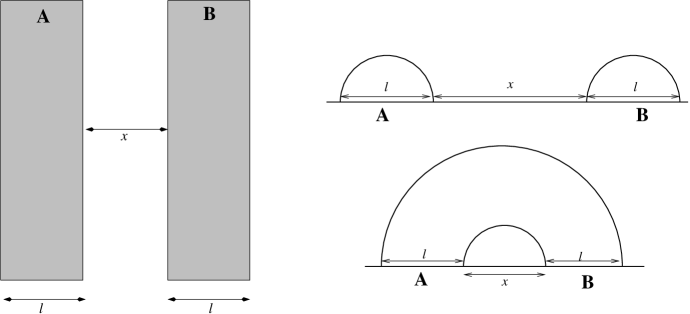
Figure 1: Two parallel disjoint strip subsystems of width $l$ and separation $x$ (and longitudinal size $V_{d-2}$) (left), with the disconnected extremal surface (top right) and the connected extremal surface (bottom right).

Mutual information is defined for two disjoint subsystems $A$ and $B$ as

$$I[A,B]=S[A]+S[B]-S[A\cup B]\ .$$ (15)

It is a measure of the correlation (both classical and quantum) between the degrees of freedom of two disjoint subsystems $A$ and $B$. Mutual information is finite, positive semi-definite, and proportional to entanglement entropy when $B\equiv A^{c}$ (in that case, $S(A\cup A^{c})=0$). This linear combination of entanglement entropies ensures that the short distance area law divergence cancels between the various individual terms rendering the mutual information finite. There is a new cutoff-independent divergence however that arises when the two subsystems approach each other and collide, as we will see below.

The holographic prescription of Ryu-Takayanagi implies in a simple geometric way that mutual information vanishes when the two subsystems are widely separated: thus as discussed in [15], mutual information undergoes a disentangling phase transition as the separation between the two striplike subsystems $A$ and $B$ increases. Recall that we choose that extremal surface which has minimal area, given the boundary conditions defined by the subsystem in question. In the case of the subsystem $A\cup B$ defined by two disjoint strips, there are two candidate extremal surfaces as in Figure 1. When the two subsystems are widely separated, the relevant extremal surface with lower area is simply the union of the two disconnected surfaces so that $S[A\cup B]=S[A]+S[B]$. However for nearby subsystems, the connected surface has lower area. For simplicity, we consider two disjoint parallel strip subsystems with longitudinal size $V_{d-2}$, and of the same width $l$ each, with separation $x$. For fixed width $l$, we can vary the separation $x$. Then as we vary ${x\over l}$ which is a dimensionless parameter, the behaviour of the extremal surface and its area $S[A\cup B]$ change: the extremal surface is

$$(i) \mbox{the disconnected surface:\ area}\ \ S[A\cup B]=S(A)+S(B)=2S(l)\ ,\ \ \mbox{for large}\ \ {x\over l}\ ,$$ (16)

$$(ii) \mbox{the connected surface:\ area}\ \ S[A\cup B]=S(2l+x)+S(x)\ ,\ \ \mbox{for small}\ \ {x\over l}\ .$$

The Ryu-Takayanagi prescription of choosing the extremal surface of minimal area then leads to a change in the entangling surface for the combined subsystem $A\cup B$. Correspondingly the mutual information changes as

$$I[A,B] >\ 0,\qquad\qquad\qquad{x\over l}\ <\ {x_{c}\over l}\ ,$$ (17)

$$=\ 0,\qquad\qquad\qquad{x\over l}\ >\ {x_{c}\over l}\ .$$

The critical value ${x_{c}\over l}$ is a dimensionless number, and depends on the field theory in question as well on the CFT state, as we discuss below. This critical value ${x_{c}\over l}$ is thus the location of a sharp disentangling transition in the classical gravity approximation, since the mutual information vanishes for larger separations implying the subsystems are uncorrelated, especially in light of an interesting relation between the mutual information and correlation functions. It is known [30] that $I[A,B]$ sets an upper bound for 2-point correlation functions of operators, with one insertion at a point in region $A$ and the other in $B$,

$$I[A,B]\geq\frac{(\langle{\cal O}_{A}{\cal O}_{B}\rangle-\langle{\cal O}_{A}\rangle\langle{\cal O}_{B}\rangle)^{2}}{2|{\cal O}_{A}|^{2}|{\cal O}_{B}|^{2}}\ .$$ (18)

This inequality implies that beyond the disentangling transition point all 2-point correlation functions also vanish (with one point in $A$ and the other in $B$), since the mutual information vanishes. It is important to note that entanglement entropy and mutual information via the Ryu-Takayanagi prescription are $O(N^{2})$ observables in the classical gravity approximation. However the 2-pt correlators are normalized as $O(1)$. One might imagine the mutual information decays as $I[A,B]\sim\sum{c_{\Delta}\over r_{A,B}^{4\Delta}}$ and indeed the quantum $O(1)$ contributions effectively give a long distance expansion for mutual information [31] (see also [15] [32] [10] [33]). However the coefficients $c_{\Delta}$ at the classical level $O(N^{2})$ vanish: this shows up in the large $N$ approximation as the sharp disentangling transition in mutual information.

We now discuss this for large $N$ conformal field theories in the ground and excited states. For the ground state, the mutual information for two strip shaped subsystems of width $l$ parallel to each other and with separation $x$ is

$$I[A,B]\ =\ -cV_{d-2}\left({2\over l^{d-2}}-{1\over(2l+x)^{d-2}}-{1\over x^{d-2}}\right)=\ -c{V_{d-2}\over l^{d-2}}\left(2-{1\over(2+{x\over l})^{d-2}}-{1\over({x\over l})^{d-2}}\right).$$ (19)

This arises from the cutoff-independent parts of entanglement, the divergent terms cancelling. We see that for small separation $x$, the mutual information $I[A,B]$ grows as $I[A,B]\sim{V_{d-2}\over x^{d-2}}$ and exhibits a divergence as $x\rightarrow 0$, i.e. when the subsystems collide with each other. As ${x\over l}$ increases, $I[A,B]$ decreases and then vanishes at a critical value of ${x\over l}$. Beyond this critical separation, the expression (19) for $I[A,B]$ as it stands is negative and is meaningless: this simply reflects the fact that the correct extremal surface for $A\cup B$ is in fact the disconnected surface, i.e. the subsystems disentangle, and mutual information actually vanishes beyond the disentangling point. This disentangling transition can be identified as the zero of $I[A,B]$ above, giving  ${x_{c}\over l}\simeq 0.732\ [d=4]$, and $0.62\ [d=3]$, and so on.

Such a disentangling transition also happens at finite temperature, but the phase diagram is more complicated and has nontrivial dependence on the length scale ${1\over T}$ set by the temperature $T$. For $l,x\ll{1\over T}$, i.e. subsystem widths and separation small relative to the temperature scale, we only expect small corrections to the ground state behaviour above. Thus the disentangling transition point occurs at values which are “near” those for the ground state. However for large width $l$, the entanglement is well approximated by the extensive (linear) thermal entropy: thus

$$I[A,B]\sim\ T^{d-1}V_{d-2}\ \left(2l-(2l+x)-S^{fin}(x)\right)=\ T^{d-1}V_{d-2}\ \left(-S^{fin}(x)\ -\ x\right).$$ (20)

Thus we see that as the separation $x$ increases, $-S^{fin}(x)>0$ decreases and $I[A,B]$ decreases and eventually vanishes at a critical $x_{c}$, which turns out to be smaller in value than for the ground state. When the thermal entropy dominates the entanglement or equivalently the subsystem widths and separation are both large relative to the temperature scale, we see that

$$I[A,B]\sim\ T^{d-1}V_{d-2}\ \left(2l-(2l+x)-x\right)=-2T^{d-1}V_{d-2}x\ ,$$ (21)

which is negative. This is a reflection of the fact that the two subsystems in fact are completely disentangled for any separation $x$ larger than ${1\over T}$. In some sense, the temperature “disorders” the system and the subsystems disentangle faster at finite temperature than in the ground state.

In what follows, we analyse holographic mutual information for $AdS$ plane waves. We will see some similarities with the finite temperature case, but with nontrivial phase structure depending on the scale $Q^{-1/d}$. There are however some key differences as we will see below.

5 Mutual information in $AdS$ plane waves

$AdS$ plane waves exhibit anisotropy due to the energy flux in one direction. We are considering parallel disjoint strip subsystems that are either both along the flux or both orthogonal to the flux. We can analyse mutual information in two extreme regimes, where the strip widths $l$ are large or small compared to the length scale set by the energy density flux $Q$. Eventually we will carry out some numerical analysis in intermediate regimes as well.

5.1 Wide strips: $lQ^{1/d}\gg 1$

Consider first the strip along the energy flux direction, with width direction along say $x_{1}$ (we assume $d\geq 3$). Then the spacelike strip subsystem $A$ lying on a constant time slice has $0\leq x_{1}\leq l,\ (x^{+},x^{-})=(\alpha y,-\beta y)=(y,-y),\ -\infty<y,x_{2},x_{3},\cdots,x_{d-2}<\infty$. The extremal surface $\gamma_{A}$ is specified by the function $x_{1}=x(r)$. $V_{d-2}$ denotes the volume in the $y$ and $(x_{2},\cdots,x_{d-2})$ direction. $\epsilon$ is the UV cutoff. The subsystem width in terms of the turning point $r_{*}$ is [13]

$$\Delta x_{1}=l=2\int^{r_{*}}_{0}dr\frac{Ar^{d-1}}{\sqrt{2+Qr^{d}-A^{2}r^{2(d-1)}}}\ ,$$ (22)

while the entanglement entropy in terms of the area functional is

$$S_{A}={Area\over 4G_{d+1}}={2V_{d-2}R^{d-1}\over 4G_{d+1}}\int^{r_{*}}_{\epsilon}\frac{dr}{r^{d-1}}\frac{2+Qr^{d}}{\sqrt{2+Qr^{d}-A^{2}r^{2(d-1)}}}\ .$$ (23)

There is a leading area law divergence from the contribution near the boundary $r=\epsilon$, with $EE\sim\ N^{2}{V_{d-2}\over\epsilon^{d-2}}$ , where we have used $N^{2}\sim{R^{d-1}\over G_{d+1}}$. For large energy density $Q$, and large width $l$, the turning point equation $2+Qr_{*}^{d}-A^{2}r_{*}^{2d-2}=0$ can be approximated as $Qr_{*}^{d}\simeq A^{2}r_{*}^{2(d-1)}\gg 1$, so that $l\sim r_{*}$ from (22). The finite cutoff-independent piece of $S_{A}$ is then estimated as

$$S_{A}^{finite} \sim \pm{R^{d-1}\over G_{d+1}}V_{d-2}\sqrt{Q}\ l^{2-\frac{d}{2}}\qquad\ \ [d\neq 4]$$ (24)

$$\sim N^{2}V_{2}\sqrt{Q}\ \log(lQ^{1/4})\qquad\ \ [d=4]\ .$$ (25)

The sign in front of (24) is $+$ for $d<4$ and $-$ for $d>4$.

Towards estimating mutual information for $AdS$ plane waves, we must note that there are multiple regimes stemming from the various length scales $l,\ x,\ Q^{-1/d}$. When the strip widths and separations are large relative to the correlation length, i.e. $lQ^{1/d}\gg 1$ and $xQ^{1/d}\gg 1$, we can use the above estimates for the finite parts of entanglement entropy to estimate mutual information. For the $AdS_{5}$ plane wave, when the strips are not too far apart, we can assume mutual information is nonzero, obtaining from the finite parts above,

$$I[A,B]=2S^{fin}(l)-S^{fin}(2l+x)-S^{fin}(x)\sim\ V_{2}\sqrt{Q}\log\left({l^{2}\over x(2l+x)}\right).$$ (26)

The argument of the logarithm vanishes when

$$I[A,B]\rightarrow 0\qquad\Rightarrow\qquad l^{2}=2lx+x^{2},\qquad{\it i.e.}\ \ \ {x_{c}\over l}=\sqrt{2}-1\simeq 0.414\ .$$ (27)

Thus the subsystems disentangle at a separation less than that for the $AdS_{5}$ ground state, which has ${x_{c}\over l}=0.732$. It is also noteworthy that for any large $Q$, the subsystems disentangle only when they are sufficiently wide apart in comparison with the width, i.e. $x\geq 0.414l$, independent of the characteristic energy scale $Q^{-1/4}$: in particular the disentangling point $x_{c}$ here could be substantially bigger than $Q^{-1/4}$. This transition location agrees with the analysis for hyperscaling violating spacetimes in [10] and [21], in accordance with the fact that the $AdS_{5}$ plane wave gives rise to the corresponding hyperscaling violating spacetime. The strips, being parallel to the flux, are unaffected by the reduction along the $x^{+}$-circle from that perspective. In the present case, we are studying this entirely from the higher dimensional $AdS$ plane wave point of view. Note that this is quite distinct from the finite temperature case [21] in the corresponding regime $lT\gg 1,\ xT\gg 1$, i.e. sizes larger than the temperature scale ${1\over T}$ : in that case, the linear extensive growth of entanglement in this regime implied that the subsystems disentangled for any finite separation $x$ independent of the width $l$ (21).

Strictly speaking, we are thinking of the regulated $AdS$ plane wave as a limit of the highly boosted low temperature $AdS$ black brane, with a large separation of scales $Q\gg r_{0}^{4}$ between the energy density $Q=\lambda^{2}r_{0}^{4}$ and the temperature $r_{0}$, with $\lambda$ being the boost parameter. Over this wide range of length scales, the physics is dominated by the $AdS$ plane wave description, with departures arising in the far infrared where the black brane horizon physics enters as a regulator. From this point of view, we are thinking of the strip subsystem widths as satisfying $Q^{-1/4}\ll l\ll{1\over r_{0}}$, with the above behaviour of mutual information holding correpondingly: in the far IR when $l\gg{1\over r_{0}}$ the behaviour of mutual information resembles that in the finite temperature case.

A similar analysis can be done for the $AdS_{4}$ plane wave, in the regime $lQ^{1/3}\gg 1$ and $xQ^{1/3}\gg 1$, taking again for simplicity both strips of equal width $l$ with separation $x$. Then the mutual information arises from the finite parts of entanglement estimated (24) for large $Q$ giving

$$I[A,B]\sim\ V_{1}\sqrt{Q}\left(2\sqrt{l}-\sqrt{2l+x}-\sqrt{x}\right).$$ (28)

This decreases as the separation $x$ increases and finally vanishes when

$$I[A,B]\rightarrow 0\qquad\Rightarrow\qquad{x_{c}\over l}={1\over 4}\ ,$$ (29)

which is the location of the disentangling transition in this regime. Again we see that the subsystems disentangle when they are sufficiently wide apart in comparison to their widths $l$, without specific dependence on the energy scale $Q^{-1/3}$ as for the $AdS_{5}$ plane wave discussed above.

Nonconformal D-brane plane waves and entanglement entropy were studied in [14], with the emerging picture and scalings consistent with $AdS$ plane waves in cases where comparison is possible. The analysis is more complicated in the nonconformal cases since there are multiple different length scales in the phase diagram. The structure of mutual information is still further complicated and we will not carry out a systematic study here. We can however make some coarse estimates in the large flux regime. For instance the D2-M2 ground state phase diagram [28] extends to a corresponding one for the D2-brane plane waves. The finite part of EE for a strip along the flux in the D2-brane supergravity regime is $S^{fin}_{D2}\sim\ V_{1}\sqrt{Q}\sqrt{l}\sqrt{N_{eff}(l)}\sim\ V_{1}\sqrt{Q}\sqrt{l}\sqrt{{N^{2}\over(g_{YM}^{2}Nl)^{1/3}}}\propto l^{1/3}$. Noting the D2-sugra regime of validity, it can be seen that this finite part is greater than $V_{1}\sqrt{Q}\sqrt{l}\sqrt{N^{3/2}}$ for the M2-brane ($AdS_{4}$) plane wave arising in the far IR [14]. In the D2-regime, we can approximate the mutual information as $MI_{D2}\sim\ V_{1}\sqrt{Q}(2l^{1/3}-(2l+x)^{1/3}-x^{1/3})$ which shows a disentangling transition at ${x_{c}\over l}\sim 0.31$. Recalling that for the M2-brane regime, we have ${x_{c}\over l}\sim 0.25$, we see that $x_{c}$ decreases along the RG flow from the D2-brane sugra to the M2-brane regime. Similarly for the ground states also, it can be checked that in the D2-regime, we have ${x_{c}\over l}\sim 0.66$ while in the M2-regime, we have ${x_{c}\over l}\sim 0.62$. It is unclear if these are indications of some deeper structure for the “flow” of mutual information.

Now we make a few comments on mutual information in the case where the strips are orthogonal to the energy flux. In the large flux regime, we know [13] that entanglement entropy shows a phase transition for $l\gg Q^{-1/d}$ with no connected extremal surface but only disconnected ones. In this regime, we expect that mutual information simply vanishes since the connected surface of mutual information (16) is already disconnected: thus the entanglement is saturated for each of $S[l],S[2l+x],S[x]\sim S_{sat}$ so that $MI\sim 2S(l)-S[2l+x]-S[x]=0$. In sec. 5.3, we will study entanglement and mutual information in the perturbative regime $Ql^{d}\ll 1$: however in this regime, we do not expect any signature of the phase transition which is only visible for wide strips. It is then reasonable to expect some interesting interplay between the phase transition and the location of the disentangling transition for mutual information.

5.2 Narrow strips: $lQ^{1/d}\ll 1$,  strips along flux

We would now like to understand the case of narrow strips, i.e. with the dimensionless quantity $lQ^{1/d}\ll 1$. In this limit, we expect that the entanglement entropy is only a small departure from the pure $AdS$ case, since the energy density flux $Q$ will only make a small correction to the ground state entanglement. We will first analyse the strip along the flux and obtain the entanglement correction to the ground state. This has parallels with “entanglement thermodynamics” [17] [19] [20] for these $AdS$ plane waves, treating the $g_{++}$ mode as a small deformation to $AdS$.

In the limit $Q^{1/d}l\ll 1$, we first calculate the change in the turning point $r_{*}$ upto $O(Q)$, and then expand the width integral and area integral around $AdS_{d+1}$, using (22), (23). First we note that the pure $AdS$ case, with $s$ the turning point of the minimal surface, has the width integral

$$l=2\int_{0}^{s}\frac{A}{\sqrt{\frac{2}{r^{2(d-1)}}-A^{2}}}=2\int_{0}^{s}dr\frac{(r/s)^{d-1}}{\sqrt{1-\left(\frac{r}{s}\right)^{2(d-1)}}}=2\left(\frac{\sqrt{\pi}\Gamma\left(\frac{d}{2d-2}\right)}{\Gamma\left(\frac{1}{2d-2}\right)}\right)s\ \equiv\ 2\eta s\ ,$$ (30)

using $A^{2}=\frac{2}{s^{d-1}}$ and $\eta=\int_{0}^{1}\frac{x^{d-1}}{\sqrt{1-x^{2(d-1)}}}dx$. We want to calculate the change in the ground state entanglement entropy under the $AdS$ plane wave perturbation to $O(Q)$, with the strip along the flux. With the entangling surface fixed at width $l$, the turning point $s$ now changes to $r_{*}=s+\delta r_{*}$. We recast (22) and the turning point equation as

$$\frac{l}{2}=\int_{0}^{r_{*}}dr\frac{A}{\sqrt{\frac{g(r)}{r^{2(d-1)}}-A^{2}}}\quad\mbox{with}\quad g(r)=2+Qr^{d}\ ,\quad\mbox{and}\quad A^{2}=\frac{g(r_{*})}{r_{*}^{2(d-1)}}\equiv\frac{g_{*}}{r_{*}^{2(d-1)}}\ .$$ (31)

Then we obtain

$$\frac{l}{2}=\int_{0}^{r_{*}}dr\frac{\frac{\sqrt{g_{*}}}{r_{*}^{d-1}}}{\frac{1}{r^{d-1}}\sqrt{g(r)-{g_{*}}\left(\frac{r}{r_{*}}\right)^{2(d-1)}}}\ =\ \int_{0}^{r_{*}}dr\frac{(r/r_{*})^{d-1}}{f(r,r_{*})}\frac{\left(1+\frac{Qr_{*}^{d}}{4}\right)}{\sqrt{1+\frac{Qr^{d}-Qr_{*}^{d}\left(\frac{r}{r_{*}}\right)^{2(d-1)}}{2f^{2}(r,r_{*})}}}\ ,$$ (32)

with the function

$$f(r,r_{*})=\sqrt{1-\left(\frac{r}{r_{*}}\right)^{2(d-1)}}\ ,\qquad\quad 0<f(r,r_{*})<1\quad\ \mbox{for all}\ r<r_{*}\ .$$ (33)

The above expression has been obtained by taking $Qr_{*}^{d}\ll 1$ and expanding out the integrand. The above width integral can be further simplified to $O(Q)$ as

$$\frac{l}{2} = \int_{0}^{r_{*}}dr\frac{(r/r_{*})^{d-1}}{f(r,r_{*})}{\left(1+\frac{Qr_{*}^{d}}{4}\right)}\left({1-\frac{Qr^{d}-Qr_{*}^{d}\left(\frac{r}{r_{*}}\right)^{2(d-1)}}{4f^{2}(r,r_{*})}}\right)$$ (34)

$$= \int_{0}^{r_{*}}dr\frac{(r/r_{*})^{d-1}}{f(r,r_{*})}\left(1+\frac{Q}{4f^{2}(r,r_{*})}(r_{*}^{d}-r^{d})\right)=\ s\eta=(r_{*}-\delta r_{*})\eta\ ,$$

the last expression arising since the width $l$ is as in $AdS$. Using (30), we see that the leading $AdS$ piece cancels giving

$$\delta r_{*}=-\frac{Q}{4\eta}\int_{0}^{r_{*}}dr\frac{(r/r_{*})^{d-1}}{f^{3}(r,r_{*})}\Big{(}r_{*}^{d}-r^{d}\Big{)}\sim\ -\frac{Qs^{d+1}}{4\eta}\int_{0}^{1}dx\frac{x^{d-1}(1-x^{d})}{(1-x^{2(d-1)})^{3/2}}\ .$$ (35)

As $r_{*}$ happens to be the turning point of the minimal surface, $r<r_{*}$ which implies that $\delta r_{*}<0$ always. Also since $\delta r_{*}$ is $O(Q)$, we have approximated $r_{*}\sim s$ to obtain the second expression. Thus

$$\delta r_{*}\sim\ -\frac{Qs^{d+1}}{4\eta}\frac{\sqrt{\pi}}{(d-1)^{2}}\left(\frac{\Gamma(\frac{1}{d-1})}{\Gamma(\frac{1}{2}+\frac{1}{d-1})}-(d-1)\frac{\Gamma(\frac{d}{2d-2})}{\Gamma(\frac{1}{2d-2})}\right)\equiv\ -\frac{Qr_{*}^{d+1}}{4\eta}{\cal N}_{r_{*}}\ .$$ (36)

We now calculate the change in the area integral and correspondingly the entanglement entropy upto $O(Q)$. For pure $AdS$, i.e. the CFT ground state, we have

$$4G_{d+1}S_{0}=2V_{d-2}R^{d-1}\int_{0}^{s}\frac{dr}{r^{d-1}}\frac{1}{f(r,s)}\ ,$$ (37)

with $f(r,s)=\sqrt{1-\left(\frac{r}{s}\right)^{2(d-1)}}$ as in (33). We focus on the finite part of the above integral and use $l=2s\eta$, obtaining

$$4G_{d+1}S_{0}\ =\ \#R^{d-1}{V_{d-2}\over\epsilon^{d-2}}\ -\ \frac{2^{d-1}\pi^{\frac{d-1}{2}}}{(d-2)}\left(\frac{\Gamma(\frac{d}{2d-2})}{\Gamma(\frac{1}{2d-2})}\right)^{d-1}{V_{d-2}\over l^{d-2}}R^{d-1}\ .$$ (38)

In our case of the $AdS_{d+1}$ plane wave,

$$4G_{d+1}S=2V_{d-2}R^{d-1}\int_{0}^{r_{*}}\frac{dr}{r^{d-1}}\frac{2+Qr^{d}}{\sqrt{2+Qr^{d}-A^{2}r^{2(d-1)}}}$$ (39)

Treating this as an infinitesimal $g_{++}$-deformation and expanding around pure $AdS$, we would like to obtain the $O(Q)$ change in EE, or equivalently the infinitesimal change for the plane wave excited state relative to the ground state. From the turning point equation, we have $A^{2}=\frac{2+Qr_{*}^{d}}{r_{*}^{2(d-1)}}$ as before, giving

$$4G_{d+1}S = 2V_{d-2}R^{d-1}\int_{0}^{r_{*}}\frac{dr}{r^{d-1}}\frac{2+Qr^{d}}{\sqrt{2\Big{(}1-\Big{(}\frac{r}{r_{*}}\Big{)}^{2(d-1)}\Big{)}+Qr^{d}-Qr_{*}^{d}\Big{(}\frac{r}{r_{*}}\Big{)}^{2(d-1)}}}$$ (40)

$$= 2\sqrt{2}V_{d-2}R^{d-1}\int_{0}^{r_{*}}\frac{dr}{r^{d-1}}\frac{1}{f(r,r_{*})}\left(1+\frac{Qr^{d}}{2}\right)\left(1-\frac{Qr^{d}-Qr_{*}^{d}\left(\frac{r}{r_{*}}\right)^{2(d-1)}}{4f(r,r_{*})^{2}}\right)$$

$$= 4G_{d+1}S_{0}\ +\ 2\sqrt{2}R^{d-1}{\cal N}_{EE}\ V_{d-2}Qr_{*}^{2}\ ,$$

where

$${\cal N}_{EE} =\int_{0}^{1}dx\left[\frac{x}{2\sqrt{1-x^{2(d-1)}}}+\frac{1}{4x^{d-1}\sqrt{1-x^{2(d-1)}}}\left(\frac{(1-x^{d})}{(1-x^{2(d-1)})}-1\right)\right]$$ (41)

$$=\ \frac{\sqrt{\pi}}{8(d-1)^{2}}\left(\frac{(d+1)\Gamma(\frac{1}{d-1})}{\Gamma(\frac{1}{2}+\frac{1}{d-1})}-\frac{2(d-1)\Gamma(\frac{d}{2d-2})}{\Gamma(\frac{1}{2d-2})}\right)\ .$$

It can be checked that the constant ${\cal N}_{EE}$ is positive, so that the correction to the entanglement entropy is positive. To $O(Q)$, we can replace $r_{*}$ by $s$, the pure $AdS$ turning point. Then using $l=2s\eta$, we see that

$$\Delta S\sim\ +{R^{d-1}\over G_{d+1}}{{\cal N}_{EE}\over 4\eta^{2}\sqrt{2}}\ V_{d-2}Ql^{2}\ =+{R^{d-1}\over G_{d+1}}{{\cal N}_{EE}\over 4\eta^{2}\sqrt{2}}\ {V_{d-2}\over l^{d-2}}(Ql^{d})\ ,$$ (42)

with $Ql^{d}\ll 1$. There are parallels of this analysis with “entanglement thermodynamics” [17, 19, 20] (see also [34, 35, 36]). In the present case, we have the energy change in the strip $\Delta E\sim\int\delta T_{tt}d^{d-1}x\sim\ QV_{d-2}l$, giving $T_{E}\Delta S_{E}\sim\Delta E$ with the “entanglement temperature” $T_{E}\sim{1\over l}$ . There is also an entanglement pressure. Although it is not crucial for our purposes here, it would be interesting to develop this further.

The above entanglement entropy change implies that the change in mutual information is negative (with $I_{0}[A,B]$ the mutual information in pure $AdS$):

$$I[A,B] = I_{0}[A,B]\ +\ \Delta I[A,B]\ =\ I_{0}[A,B]\ +\ {R^{d-1}\over G_{d+1}}{{\cal N}_{EE}\over\sqrt{2}}\ V_{d-2}Q\left(2l^{2}-(2l+x)^{2}-x^{2}\right)$$ (43)

$$= I_{0}[A,B]\ -\ 2{R^{d-1}\over G_{d+1}}{{\cal N}_{EE}\over 4\eta^{2}\sqrt{2}}\ V_{d-2}Ql^{2}\ \left(1+{x\over l}\right)^{2}\ .$$

Thus we see that mutual information strictly decreases, for a small $T_{++}$ energy density flux perturbation along the strip subsystem. In this perturbative regime with the correction scaling as $O(Q)$ and as the area of the interface $V_{d-2}$, the entanglement and mutual information corrections involve the dimensionless quantity $V_{d-2}Ql^{2}$.

It is worth noting that unlike in the wide strip regime (26), the disentangling transition in this perturbative regime certainly depends on the energy density $Q$ and the strip width through $Ql^{d}$. In particular, using (38), (19), we see that the mutual information (43) vanishes at

$${\cal N}^{0}_{EE}\Big{(}{1\over({x\over l})^{d-2}}+{1\over(2+{x\over l})^{d-2}}-2\Big{)}-{{\cal N}_{EE}\over 2\sqrt{2}\eta^{2}}Ql^{d}\Big{(}1+{x\over l}\Big{)}^{2}=0\ ,$$ (44)

where ${\cal N}^{0}_{EE}$ is the constant coefficient of the finite part in (38). A numerical study later (sec. 5.4) describes the location of the vanishing of mutual information and the disentangling transition for intermediate regimes as well, where $Ql^{d}\sim O(1)$.

5.3 Narrow strips: $lQ^{1/d}\ll 1$, strips orthogonal to flux

We describe the change in entanglement entropy and mutual information for the strips orthogonal to the flux in the perturbative regime $lQ^{1/d}\ll 1$ here. The analysis is similar to the previous case, but involves more calculation.

We first consider a single strip and study entanglement. In this case, the width direction of the strip $A$ is parallel to $x_{d-1}$, with $x^{\pm}=\frac{t\pm x_{d-1}}{\sqrt{2}}$. The bulk extremal surface $\gamma_{A}$ is specified by $x^{+}=x^{+}(r),\ x^{-}=x^{-}(r)$, and the spacelike strip subsystem has width

$$\Delta x^{+}=-\Delta x^{-}=\frac{l}{\sqrt{2}}>0\ ,$$ (45)

(spacelike implying $\Delta t=0$) and longitudinal size $V_{d-2}\sim L^{d-2}$ with $L\gg l$ in the $x_{i}$ directions. $\epsilon$ is the UV cut-off. Then the width integrals and the entanglement entropy area functional reduce to [13]

$$\frac{\Delta x^{+}}{2}=\int^{r_{*}}_{0}\frac{dr}{\sqrt{\frac{A^{2}B^{2}}{r^{2(d-1)}}+Qr^{d}-2B}}\ ,\qquad\frac{\Delta x^{-}}{2}=\int^{r_{*}}_{0}\frac{(Qr^{d}-B)\ dr}{\sqrt{\frac{A^{2}B^{2}}{r^{2(d-1)}}+Qr^{d}-2B}}\ ,$$ (47)

$$S_{A}\ =\ {2R^{d-1}V_{d-2}\over 4G_{d+1}}\int^{r_{*}}_{\epsilon}\frac{dr}{r^{d-1}}\frac{AB}{\sqrt{A^{2}B^{2}-2Br^{2(d-1)}+Qr^{3d-2}}}\ .$$

Unlike the previous case, here we have two parameters $A,B$ and two integrals specifying the subsystem width $l$ as a function of the turning point $r_{*}$ of the extremal surface, given by (47). For pure $AdS$, with $Q=0$, (47) alongwith (45) fixes $B=1$, with $x^{\pm}$ treated “symmetrically” as expected in the absence of the energy flux. We will treat the $AdS$ plane wave case in $O(Q)$ perturbation theory and expand both integrals around $AdS$. The turning point equation here is

$$\frac{A^{2}B^{2}}{r_{*}^{2(d-1)}}+Qr_{*}^{d}-2B=0\qquad\Rightarrow\qquad\frac{A^{2}B^{2}}{r^{2(d-1)}}=\left(\frac{r_{*}}{r}\right)^{2(d-1)}(2B-Qr_{*}^{d})\ .$$ (48)

This recasts the denominator of the width integrals in terms of $f(r,r_{*})=\sqrt{1-\left(\frac{r}{r_{*}}\right)^{2(d-1)}}$ and $B$ alone,

$$\left[\frac{A^{2}B^{2}}{r^{2(d-1)}}+Qr^{d}-2B\right]^{1/2}=\left(\frac{r_{*}}{r}\right)^{d-1}f(r,r_{*})\sqrt{2B}\left[1-\frac{Qr_{*}^{d}\Big{(}1-\big{(}\frac{r}{r_{*}}\big{)}^{3d-2}\Big{)}}{2Bf^{2}}\right]^{1/2}.$$ (49)

However unlike (31) earlier, we are still left with the parameter $B$ here, so the turning point equation does not suffice. The other relation for recasting both $A$ and $B$ in terms of $Q,r_{*}$ comes from the fact that we have a space-like subsystem, i.e. (45). Specifically with the pure $AdS$ case corresponding to $B=1$, in this perturbative regime with $Ql^{d}\ll 1$, we can safely assume that $B=1+\Delta B$ with $\Delta B\sim O(Q)$. Since the two width integrals for $\Delta x^{+}$ and $\Delta x^{-}$ must obey the equality $\Delta x^{+}=-\Delta x^{-}={l\over\sqrt{2}}$, we must have that the change in the turning point $\delta r_{*}$ obtained from both is the same, which fixes $\Delta B\propto Qr_{*}^{d}$ as we will see.

To elaborate, from (45), (47), (49), we have

$$\frac{\Delta x^{+}}{\sqrt{2}}\ =\ \frac{l}{2}\ =\ \int_{0}^{r_{*}}dr\frac{(r/r_{*})^{d-1}}{f(r,r_{*})\sqrt{B}}\frac{1}{\left[1-\frac{Qr_{*}^{d}\left(1-(r/r_{*})^{3d-2}\right)}{2Bf^{2}}\right]^{1/2}}\ .$$ (50)

Now, with $B=1+\Delta B=1+O(Q)$, we can expand this to $O(Q)$ obtaining

$$\frac{l}{2}=\int_{0}^{r_{*}}dr\frac{(r/r_{*})^{d-1}}{f(r,r_{*})}-\frac{\Delta B}{2}\int_{0}^{r_{*}}dr\frac{(r/r_{*})^{d-1}}{f(r,r_{*})}+Qr_{*}^{d}\int_{0}^{r_{*}}dr\frac{(r/r_{*})^{d-1}(1-(r/r_{*})^{3d-2})}{4f^{3}(r,r_{*})}\ .$$ (51)

As in the previous subsection, we keep our entangling surface fixed so $l=2s\eta$, with $s$ the pure $AdS$ turning point. The new turning point is $r_{*}=s+\delta r_{*}$, so $l/2=r_{*}\eta-\delta r_{*}\eta$. Thus

$$-\delta r_{*}\eta=-\frac{\Delta Br_{*}}{2}\int_{0}^{1}dx\frac{x^{d-1}}{\sqrt{1-x^{2(d-1)}}}+Qr_{*}^{d+1}\int_{0}^{1}dx\frac{x^{d-1}(1-x^{3d-2})}{4(1-x^{2(d-1)})^{3/2}}\ .$$ (52)

Starting with the $\Delta x^{-}$ integral and using (45), (47), (49), we have analogous to (50),

$$\frac{l}{2}=\int_{0}^{r_{*}}dr\frac{(r/r_{*})^{d-1}}{f(r,r_{*})}\frac{B-Qr^{d}}{\sqrt{B}\Big{(}1-\frac{Qr_{*}^{d}\left(1-(r/r_{*})^{3d-2}\right)}{2Bf^{2}}\Big{)}^{1/2}}\ .$$ (53)

As above, expanding to $O(Q)$ gives

$$\frac{l}{2}=\int_{0}^{r_{*}}dr\frac{(r/r_{*})^{d-1}}{f(r,r_{*})} +\frac{\Delta B}{2}\int_{0}^{r_{*}}dr\frac{(r/r_{*})^{d-1}}{f(r,r_{*})}$$ (54)

$$+Qr_{*}^{d}\int_{0}^{r_{*}}dr\frac{(r/r_{*})^{d-1}(1-(r/r_{*})^{3d-2})}{4f^{3}(r,r_{*})}-Q\int_{0}^{r_{*}}dr\frac{r^{d}(r/r_{*})^{d-1}}{f(r,r_{*})}\ .$$

Then as above, the change in turning point is given by

$$-\delta r_{*}\eta=\frac{r_{*}\Delta B}{2}\int_{0}^{1}dx\frac{x^{d-1}}{\sqrt{1-x^{2(d-1)}}} +Qr_{*}^{d+1}\int_{0}^{1}dx\frac{x^{d-1}(1-x^{3d-2})}{4(1-x^{2(d-1)})^{3/2}}$$ (55)

$$-Qr_{*}^{d+1}\int_{0}^{1}dx\frac{x^{2d-1}}{\sqrt{1-x^{2(d-1)}}}\ .$$

For this spacelike subsystem, the above (55) should be identical to (52). Using (30), this gives

$$\Delta B=\alpha Qr_{*}^{d}\ ,\quad\mbox{with}\qquad\alpha=\frac{1}{\eta}\int_{0}^{1}dx\frac{x^{2d-1}}{\sqrt{1-x^{2(d-1)}}}=\frac{\Gamma(\frac{1}{2d-2})\Gamma(\frac{1}{d-1})}{2(d-1)^{2}\Gamma(\frac{3}{2}+\frac{1}{d-1})\Gamma(\frac{d}{2d-2})}\ .$$ (56)

Using the above, we get

$$\delta r_{*}=\beta Qr_{*}^{d+1}\ ,\qquad\mbox{with}\qquad\beta=\frac{1}{4(d-1)}-\frac{2^{\frac{1}{d-1}}}{8(d-1)^{3}\sqrt{\pi}}\frac{\Gamma(\frac{1}{2d-2})^{2}}{\Gamma(\frac{3}{2}+\frac{1}{d-1})}\ .$$ (57)

It can be checked that $\beta<0$ ($\beta\rightarrow 0^{-}$ for large $d$): thus $\delta r_{*}$ is negative.

We can do a similar perturbation for finding the $O(Q)$ change in the entanglement entropy $S_{0}$ for pure $AdS$ given by (37). In the present $AdS_{d+1}$ plane wave case with the strip orthogonal to the flux, the entanglement entropy is (47), i.e.

$$4G_{d+1}S=2V_{d-2}R^{d-1}\int_{\epsilon}^{r_{*}}\frac{dr}{r^{d-1}}\frac{AB}{r^{d-1}\sqrt{\frac{A^{2}B^{2}}{r^{2(d-1)}}+Qr^{d}-2B}}\ .$$ (58)

From the turning point equation, we know that $AB=r_{*}^{d-1}\sqrt{2B-Qr_{*}^{d}}$. With $f(r,r_{*})$ as defined before, the EE can be recast as

$$4G_{d+1}S=2V_{d-2}R^{d-1}\int_{\epsilon}^{r_{*}}\frac{dr}{r^{d-1}}\frac{\left(1-\frac{Qr_{*}^{d}}{2B}\right)^{1/2}}{f(r,r_{*})\left[1-\frac{Qr_{*}^{d}(1-(r/r_{*})^{3d-2})}{2Bf^{2}}\right]^{1/2}}\ .$$ (59)

Now with $B=1+\alpha Qr_{*}^{d}$, we see that the perturbation in EE is independent of $\Delta B$ to $O(Q)$, since $B$ appears above only as ${Q\over B}$ . Expanding $S$ to $O(Q)$, we obtain

$$4G_{d+1}S = 2V_{d-2}R^{d-1}\int_{0}^{r_{*}}\frac{dr}{r^{d-1}}\frac{1}{f(r,r_{*})}\left[1-\frac{Qr_{*}^{d}}{4}+\frac{Qr_{*}^{d}}{4f^{2}}\left(1-(r/r_{*})^{3d-2}\right)\right]$$ (60)

$$= 4G_{d+1}S_{0}+2V_{d-2}R^{d-1}Qr_{*}^{2}\int_{0}^{1}dx\left[\frac{1-x^{3d-2}}{4x^{d-1}(1-x^{2(d-1)})^{3/2}}-\frac{1}{4x^{d-1}(1-x^{2(d-1)})^{1/2}}\right]$$

$$= 4G_{d+1}S_{0}\ +\ 2V_{d-2}R^{d-1}Qr_{*}^{2}{\cal M}_{EE}\ ,$$

with

$${\cal M}_{EE}=\frac{\sqrt{\pi}}{4(d-1)^{2}}\left[\frac{\Gamma(\frac{1}{d-1})}{\Gamma(\frac{d+1}{2d-2})}-(d-1)\frac{\Gamma(\frac{d}{2d-2})}{\Gamma(\frac{1}{2d-2})}\right]\ .$$ (61)

It can be checked that ${\cal M}_{EE}>0$ for $d>1$. Thus the change in entanglement entropy is positive, as before. To $O(Q)$, we have $r_{*}\sim l$, so that as before,

$$\Delta S={R^{d-1}\over 2G_{d+1}}{{\cal M}_{EE}\over 4\eta^{2}}\ V_{d-2}Ql^{2}\ =\ {R^{d-1}\over 2G_{d+1}}{{\cal M}_{EE}\over 4\eta^{2}}\ {V_{d-2}\over l^{d-2}}(Ql^{d})\ ,$$ (62)

so that as in (43) previously, the mutual information decreases as

$$I[A,B]=I_{0}[A,B]\ -\ 2{R^{d-1}\over G_{d+1}}{{\cal M}_{EE}\over 8\eta^{2}}\ V_{d-2}Ql^{2}\ \left(1+{x\over l}\right)^{2}\ ,$$ (63)

in this perturbative regime with $Ql^{d}\ll 1$. It should not be surprising that no hint of the phase transition is visible in this perturbative regime. For subsystem size well below the characteristic length scale set by the energy density, i.e. $l\ll Q^{-1/d}$, we only expect small corrections to the ground state entanglement and mutual information structure. The phase transition on the other hand corresponds to strips much wider than the characteristic length scale. In that regime, the two integrals for $\Delta x^{\pm}$ scale rather differently so that the spacelike subsystem requirement cannot be met: this leads to the absence of a connected surface and is the reflection of a phase transition. The corresponding entanglement saturation occurs since the degrees of freedom responsible for entanglement do not straddle the boundary for long if their size $\sim O(Q^{-1/d})$ is much smaller than the subsystem width, since they enter the strip and leave.

5.4 A more complete phase diagram and some numerical analysis

In the previous subsections, we have studied entanglement entropy and mutual information for large and small $Ql^{d},Qx^{d}$. It is interesting to study the interpolation between these, including the regime where $Ql^{d},Qx^{d}$ are $O(1)$. Towards this, we perform a numerical study of the entanglement entropy integrals and thence mutual information (using Mathematica). The plots in Figure 2 and Figure 3 show the finite cutoff-independent part of entanglement entropy (black, green and blue curves) for the $AdS_{4}$ and $AdS_{5}$ plane waves, setting $Q=1,3,10$ respectively, in the case of the strip along the energy flux: the red curves are those for pure $AdS_{4}$ and $AdS_{5}$. In the numerics, the area integrals have been regulated using a small UV cutoff regulator and subtracting off the area law divergence term, we obtain the finite part.

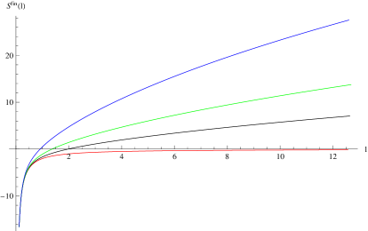
Figure 2: Plots of the finite parts of
entanglement entropy for the $AdS_{4}$ ground
state (red) and the $AdS_{4}$ plane wave (the
black, green and blue curves correspond to
the values $Q=1,3,10$ respectively).

For small $l$, we see that the $AdS$ plane wave (black, green, blue) curves lie “above” the pure $AdS$ (red) curves, which means the finite entanglement is larger than for the ground state. This is of course consistent with the previous analytic studies in the perturbative and large $Ql^{d}$ regimes but the plots show that this is also true for all $Ql^{d}$. Furthermore, the curves for larger $Q$ values lie “above” those for smaller $Q$ values, which is intuitively reasonable, implying that the finite entanglement increases with increasing energy density $Q$. The plot regions for large $l$ are in reasonable agreement with fitted curves for $\sqrt{l}$ and $\log l$ (the fits improve with increasing accuracy, number of data points etc as expected with numerics).

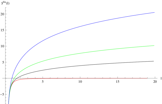
Figure 3: Plots of the finite
parts of entanglement entropy
for the $AdS_{5}$ ground state (red)
and the $AdS_{5}$ plane wave (the
black, green and blue curves
correspond to the values
$Q=1,3,10$ respectively).

Likewise, Figure 4 shows the plot of mutual information vs the separation $x$ for the $AdS_{5}$ plane wave with both strip subsystems along the flux (with fixed widths $l$ taken as $l=50$). The small $x$ region shows a growth reflecting the divergence when the subsystems approach to collide (which is similar to the divergence for pure $AdS_{5}$). The mutual information vanishes at the critical value ${x_{c}\over l}=0.41$. We have also checked that the corresponding plot for pure $AdS_{5}$ behaves as expected, with the critical value ${x_{c}\over l}\simeq 0.732$.

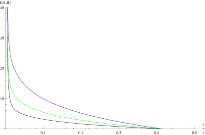
Figure 4: Plot of the mutual information
vs ${x\over l}$ with fixed width $l$ for the
$AdS_{5}$ plane wave.

Figure 5 shows the ${x\over l}$ vs $lQ^{1/d}$ parameter space (shaded regions) with nonzero mutual information for the $AdS_{5}$ plane wave with both strip subsystems along the flux. We vary the width $l$ and find the critical value $x_{c}$ holding $Q$ fixed: the three curves are for $Q=1,3,10$ as before. We see that the critical value ${x_{c}\over l}$ interpolates from about $0.732$ ($lQ^{1/d}\ll 1$, approximately $AdS_{5}$ behaviour) to $0.41$ for the $AdS_{5}$ plane wave. We see that the mutual information parameter space remains nonzero for large $lQ^{1/d}$, unlike the finite temperature case [21] where the curve has finite domain (with $x_{c}=0$ for large $lT$). We have seen previously that in the wide strip regime $Ql^{d}\gg 1$, the mutual information disentangling transition location is independent of the energy density $Q$: this is reflected in Figure 5 by the fact that the black, green, blue curves all flatten out for large $l$, signalling that the

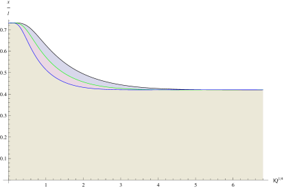
Figure 5: Plot of the ${x\over l}$ vs $lQ^{1/d}$ parameter
space with nonzero mutual information
for the $AdS_{5}$ plane wave.

critical value ${x_{c}\over l}$ is independent of the precise curve and corresponding $Q$ value. However we note that in the intermediate $Ql^{d}\sim O(1)$ regime, the mutual information disentangling transition location ${x_{c}\over l}$ certainly depends on the $Q$ value, the different curves being distinct. Thus it is only in the $Ql^{d}\gg 1$ regime that the mutual information disentangling transition becomes effectively independent of the energy flux $Q$.

There are similar plots for the $AdS_{4}$ plane wave, which we have not shown.

Our discussion so far and the corresponding plots have been for strips parallel to the energy flux. For the strips orthogonal to the flux, entanglement shows a phase transition, corroborated in the corresponding plot (shown in [13]). Plotting mutual information appears more intricate with more technical challenges in general. For wide strips $l\gtrsim Q^{-1/d}$, the strip entanglements saturate: crude plots show the strips disentangling at critical ${x_{c}\over l}$ values varying as $Q$ varies, with all ${x_{c}\over l}$ less than those for the strip along the flux (e.g. ${x_{c}\over l}\sim 0.11$ with $Q=1$, $AdS_{4}$ plane wave). It would be interesting to study this more completely.

6 Discussion

We have studied entanglement entropy and mutual information in $AdS_{d+1}$ plane waves dual to CFT excited states with energy-momentum density $T_{++}=Q$, building on [5, 13], focussing on $d=3,4$ for two strips of width $l$ and separation $x$, parallel and orthogonal to the flux.

For the strips parallel to the flux, mutual information exhibits a disentangling transition at a critical separation ${x_{c}\over l}$ less than that for the ground state. For wide strips $Ql^{d}\gg 1$, we see that the subsystems disentangle only when they are sufficiently wide apart in comparison with the width: the critical separation ${x_{c}\over l}$ is independent of the characteristic energy scale $Q^{-1/d}$ in this regime. This is quite distinct from the finite temperature case [21] where e.g. the linear extensive growth of entanglement in the corresponding regime $lT\gg 1$ implies the subsystems disentangle for any finite separation $x$ independent of $l$. For the strips orthogonal to the flux, entanglement entropy shows a phase transition for $l\gg Q^{-1/d}$ [13]: in this case, entanglement is saturated and so mutual information also vanishes. In the perturbative regime $Ql^{d}\ll 1$ for the strips both parallel and orthogonal to the flux, we have seen that the change in entanglement entropy is $\Delta S\sim+V_{d-2}Ql^{2}$ with the analysis similar to “entanglement thermodynamics”. Here the mutual information always decreases. Thus the disentangling transition in this regime again occurs for separations smaller than those for the ground state. In this perturbative regime, the critical separation ${x_{c}\over l}$ certainly depends on $Q$ and $l$. The numerical study shows the critical ${x_{c}\over l}$ has nontrivial dependence on $Q$ in intermediate regimes as well. As one approaches the wide strip regime $Ql^{d}\gg 1$, the mutual information curves approach each other and flatten out, signalling independence with $Q$.

Overall this suggests that the energy density disorders the system, so that the subsystems disentangle faster relative to the ground state. The thermal state is disordered, since in the regime with linear (extensive) entropy, the subsystems are disentangled or uncorrelated for any nonzero separation $x$. The $AdS$ plane wave states are in some sense “partially ordered”: the disentangling transition location occurs at critical values ${x_{c}\over l}$ smaller than those for the ground state for the strip along the energy flux, but the critical value remains nonzero even for wide strips $Ql^{d}\gg 1$. Perhaps this “semi-disordering” is also true for more general excited states that are “in-between” the ground and thermal states.

The $AdS_{5}$ plane wave gives rise to a hyperscaling violating spacetime exhibiting logarithmic violation of entanglement entropy, suggesting that perhaps these are indications of Fermi surfaces [9, 10]. In the regime where the strip widths and separation are large relative to the energy scale $Q^{-1/4}$, the logarithmic scaling of entanglement implies a corresponding scaling of mutual information, similar to the corresponding behaviour for Fermi surfaces. This regime is of course just one part of the full phase diagram thinking of these as simply excited states in $AdS/CFT$, as we have seen. It would be interesting to explore these further.

Acknowledgments: It is a pleasure to thank M. Rangamani, T. Takayanagi and S. Trivedi for comments on a draft, and M. Headrick for comments on a previous version of the paper. KN thanks J. Maldacena for an early conversation pertaining to a parton-like description for $AdS$ plane waves, while on a visit to the IAS, Princeton, and the IAS for hospitality over that period.

References

- [1] S. Ryu and T. Takayanagi, “Holographic derivation of entanglement entropy from AdS/CFT,” Phys. Rev. Lett. 96, 181602 (2006) [hep-th/0603001].
- [2] S. Ryu and T. Takayanagi, “Aspects of Holographic Entanglement Entropy,” JHEP 0608, 045 (2006) [hep-th/0605073].
- [3] T. Nishioka, S. Ryu and T. Takayanagi, “Holographic Entanglement Entropy: An Overview,” J. Phys. A 42 (2009) 504008; T. Takayanagi, “Entanglement Entropy from a Holographic Viewpoint,” Class. Quant. Grav. 29 (2012) 153001 [arXiv:1204.2450 [gr-qc]].
- [4] V. E. Hubeny, M. Rangamani and T. Takayanagi, “A Covariant holographic entanglement entropy proposal,” JHEP 0707 (2007) 062 [arXiv:0705.0016 [hep-th]].
- [5] K. Narayan, “On Lifshitz scaling and hyperscaling violation in string theory,” Phys. Rev. D 85, 106006 (2012) [arXiv:1202.5935 [hep-th]].
- [6] H. Singh, “Lifshitz/Schródinger Dp-branes and dynamical exponents,” JHEP 1207 (2012) 082 [arXiv:1202.6533 [hep-th]]; H. Singh, “Special limits and non-relativistic solutions,” JHEP 1012, 061 (2010) [arXiv:1009.0651 [hep-th]].
- [7] K. Narayan, “AdS null deformations with inhomogeneities,” Phys. Rev. D 86, 126004 (2012) [arXiv:1209.4348 [hep-th]].
- [8] K. Goldstein, S. Kachru, S. Prakash, S. P. Trivedi, “Holography of Charged Dilaton Black Holes,” JHEP 1008, 078 (2010) [arXiv:0911.3586 [hep-th]]; N. Iizuka, N. Kundu, P. Narayan and S. P. Trivedi, “Holographic Fermi and Non-Fermi Liquids with Transitions in Dilaton Gravity,” JHEP 1201, 094 (2012) [arXiv:1105.1162 [hep-th]]. M. Cadoni, G. D’Appollonio and P. Pani, “Phase transitions between Reissner-Nordstrom and dilatonic black holes in 4D AdS spacetime,” JHEP 1003, 100 (2010) [arXiv:0912.3520 [hep-th]]; C. Charmousis, B. Gouteraux, B. S. Kim, E. Kiritsis and R. Meyer, “Effective Holographic Theories for low-temperature condensed matter systems,” JHEP 1011, 151 (2010) [arXiv:1005.4690 [hep-th]]; E. Perlmutter, “Domain Wall Holography for Finite Temperature Scaling Solutions,” JHEP 1102, 013 (2011) [arXiv:1006.2124 [hep-th]]; B. Gouteraux and E. Kiritsis, “Generalized Holographic Quantum Criticality at Finite Density,” JHEP 1112, 036 (2011) [arXiv:1107.2116 [hep-th]]; P. Dey and S. Roy, “Lifshitz-like space-time from intersecting branes in string/M theory,” arXiv:1203.5381 [hep-th]; E. Perlmutter, “Hyperscaling violation from supergravity,” JHEP 1206, 165 (2012) [arXiv:1205.0242 [hep-th]];
- [9] N. Ogawa, T. Takayanagi and T. Ugajin, “Holographic Fermi Surfaces and Entanglement Entropy,” JHEP 1201, 125 (2012) [arXiv:1111.1023 [hep-th]].
- [10] L. Huijse, S. Sachdev and B. Swingle, “Hidden Fermi surfaces in compressible states of gauge-gravity duality,” Phys. Rev. B 85, 035121 (2012) [arXiv:1112.0573 [cond-mat.str-el]].
- [11] X. Dong, S. Harrison, S. Kachru, G. Torroba and H. Wang, “Aspects of holography for theories with hyperscaling violation,” JHEP 1206, 041 (2012) [arXiv:1201.1905 [hep-th]].
- [12] L. Bombelli, R. K. Koul, J. Lee and R. D. Sorkin, “A Quantum Source of Entropy for Black Holes,” Phys. Rev. D 34 (1986) 373; M. Srednicki, “Entropy and area,” Phys. Rev. Lett. 71 (1993) 666 [hep-th/9303048].
- [13] K. Narayan, T. Takayanagi and S. P. Trivedi, “AdS plane waves and entanglement entropy,” J. High Energy Phys. (2013), arXiv:1212.4328 [hep-th].
- [14] K. Narayan, “Non-conformal brane plane waves and entanglement entropy,” Phys. Lett. B 726, 370 (2013) [arXiv:1304.6697 [hep-th]].
- [15] M. Headrick, “Entanglement Renyi entropies in holographic theories,” Phys. Rev. D 82, 126010 (2010) [arXiv:1006.0047 [hep-th]].
- [16] B. Swingle, “Mutual information and the structure of entanglement in quantum field theory,” arXiv:1010.4038 [quant-ph].
- [17] J. Bhattacharya, M. Nozaki, T. Takayanagi and T. Ugajin, “Thermodynamical Property of Entanglement Entropy for Excited States,” Phys. Rev. Lett. 110, no. 9, 091602 (2013) [arXiv:1212.1164].
- [18] M. Nozaki, T. Numasawa and T. Takayanagi, “Holographic Local Quenches and Entanglement Density,” JHEP 1305, 080 (2013) [arXiv:1302.5703 [hep-th]].
- [19] D. Allahbakhshi, M. Alishahiha and A. Naseh, “Entanglement Thermodynamics,” JHEP 1308, 102 (2013) [arXiv:1305.2728 [hep-th]].
- [20] G. Wong, I. Klich, L. A. Pando Zayas and D. Vaman, “Entanglement Temperature and Entanglement Entropy of Excited States,” JHEP 1312, 020 (2013) [arXiv:1305.3291 [hep-th]].
- [21] W. Fischler, A. Kundu and S. Kundu, “Holographic Mutual Information at Finite Temperature,” Phys. Rev. D 87, no. 12, 126012 (2013) [arXiv:1212.4764 [hep-th]].
- [22] K. Balasubramanian and K. Narayan, “Lifshitz spacetimes from AdS null and cosmological solutions,” JHEP 1008, 014 (2010) [arXiv:1005.3291 [hep-th]].
- [23] A. Donos and J. P. Gauntlett, “Lifshitz Solutions of D=10 and D=11 supergravity,” JHEP 1012, 002 (2010) [arXiv:1008.2062 [hep-th]].
- [24] S. Kachru, X. Liu and M. Mulligan, “Gravity Duals of Lifshitz-like Fixed Points,” Phys. Rev. D 78, 106005 (2008) [arXiv:0808.1725 [hep-th]].
- [25] M. Taylor, “Non-relativistic holography,” arXiv:0812.0530 [hep-th].
- [26] J. Maldacena, D. Martelli and Y. Tachikawa, “Comments on string theory backgrounds with non-relativistic conformal symmetry,” JHEP 0810, 072 (2008) [arXiv:0807.1100 [hep-th]].
- [27] H. Casini and M. Huerta, “Entanglement and alpha entropies for a massive scalar field in two dimensions,” J. Stat. Mech. 0512:P12012,2005, [cond-mat/0511014].
- [28] N. Itzhaki, J. M. Maldacena, J. Sonnenschein and S. Yankielowicz, “Supergravity and the large N limit of theories with sixteen supercharges,” Phys. Rev. D 58, 046004 (1998) [hep-th/9802042].
- [29] J. L. F. Barbon and C. A. Fuertes, “Holographic entanglement entropy probes (non)locality,” JHEP 0804, 096 (2008) [arXiv:0803.1928 [hep-th]].
- [30] M.M. Wolf, F. Verstraete, M.B. Hastings, J.I. Cirac, “Area laws in quantum systems: mutual information and correlations”, Phys.Rev.Lett., 100, 070502 (2008), [arXiv:0704.3906].
- [31] T. Faulkner, A. Lewkowycz and J. Maldacena, “Quantum corrections to holographic entanglement entropy,” JHEP 1311, 074 (2013) [arXiv:1307.2892].
- [32] M. Van Raamsdonk, “Comments on quantum gravity and entanglement,” arXiv:0907.2939 [hep-th].
- [33] H. Casini and M. Huerta, “Remarks on the entanglement entropy for disconnected regions,” JHEP 0903, 048 (2009) [arXiv:0812.1773 [hep-th]].
- [34] D. D. Blanco, H. Casini, L. -Y. Hung and R. C. Myers, “Relative Entropy and Holography,” JHEP 1308, 060 (2013) [arXiv:1305.3182 [hep-th]].
- [35] N. Lashkari, M. B. McDermott and M. Van Raamsdonk, “Gravitational Dynamics From Entanglement ”Thermodynamics”,” JHEP 1404, 195 (2014) [arXiv:1308.3716 [hep-th]].
- [36] T. Faulkner, M. Guica, T. Hartman, R. C. Myers and M. Van Raamsdonk, “Gravitation from Entanglement in Holographic CFTs,” JHEP 1403, 051 (2014) [arXiv:1312.7856 [hep-th]].