Electroosmotic flow through a nanopore
Abstract
Electroosmotic pumping of fluid through a nanopore that traverses an insulating membrane is considered. The density of surface charge on the membrane is assumed uniform, and sufficiently low for the Poisson-Boltzmann equation to be linearized. The reciprocal theorem gives the flow rate generated by an applied weak electric field, expressed as an integral over the fluid volume. For a circular hole in a membrane of zero thickness, an analytical result is possible up to quadrature. For a membrane of arbitrary thickness, the full Poisson–Nernst–Planck–Stokes system of equations is solved numerically using a finite volume method. The numerical solution agrees with the standard analytical result for electro-osmotic flux through a long cylindrical pore when the membrane thickness is large compared to the hole diameter. When the membrane thickness is small, the flow rate agrees with that calculated using the reciprocal theorem.
keywords:
1 Introduction
A nanopore is simply a hole of small size in an impermeable membrane separating two regions containing an electrolytic buffer. A size range of 1–100 nm is fairly typical. Living cells and intracellular organelles are usually bounded by lipid membranes containing nanopores constructed of membrane-bound proteins. The transport of small molecules and polymers across such nanopores is a very common feature in living cells and is essential to their normal function (Alberts et al., 1994; Pfanner & Neupert, 1990; Matouschek et al., 2000; Martin et al., 1991; Künkele et al., 1998). Synthetic nanopores (Li et al., 2003; Storm et al., 2005a, b; Smeets et al., 2006; Hall et al., 2010; Garaj et al., 2010; Schneider et al., 2010) have been the focus of much interest in recent years following the demonstration of their use as effective single molecule sensors (Kasianowicz et al., 1996).
The main distinguishing feature of nanopore systems responsible for many of the novel effects is that their geometric dimensions are small enough so that electrokinetic effects are important. Such effects have been invoked to explain a range of observations relating to experiments involving free as well as hindered translocation of DNA across synthetic nanopores (Keyser et al., 2006; Ghosal, 2006, 2007a, 2007b; van Dorp et al., 2009; Laohakunakorn et al., 2013b). Nanopores also exhibit other unusual properties, some of which could be potentially exploited to build novel microfluidic devices. For example, conical nanopores fabricated on plastic films using the ion track-etching technique (Siwy, 2006) have been shown to exhibit ion current rectification similar to that of semiconductor diodes (Siwy & Fulinsski, 2004; Vlassiouk & Siwy, 2007; Vlassiouk et al., 2008a, b). A similar effect has been reported recently for electroosmotic flow out of nanocapillaries (Laohakunakorn et al., 2013b). A nonlinear electrokinetic effect known as Induced Charge Electroosmosis (ICEO) (Murtsovkin, 1996; Squires & Bazant, 2004) produces vortices at the edges of nanopores resembling recirculation vortices in separated flows even though the Reynolds number in such applications is essentially zero. Mixing due to these flow structures (Yossifon & Chang, 2008; Chang & Yossifon, 2009; Chang et al., 2012) together with electroconvective instabilities (Zaltzman & Rubinstein, 2007) are thought to be responsible for the “overlimiting” behaviour of the current–voltage characteristics of perm selective pores and membranes described by Rubinstein & Shtilman (1979). Similar vortical structures may be generated in cylindrical channels that undergo a sudden constriction when the relevant length scales are on the order of the Debye length (Park et al., 2006).
If an electric field is applied across an uncharged membrane, Induced Charge Electroosmosis leads to velocities with no net flow through the membrane unless symmetry is somehow broken. Molecular dynamics simulations of flow through nanopores in uncharged membranes, such as graphene sheets (Hu et al., 2012), show that differences in mobility between cations and anions can result in asymmetric Debye layers and consequent net flow through the membrane. Symmetry is also broken if the membrane is charged, so that the intrinsic field due to the membrane competes with the externally applied field in determining the distribution of ions in the Debye layer (Mao et al., 2013).
If a voltage is applied across a charged membrane containing a long narrow pore an electroosmotic flow is generated by the electric field acting on the charge cloud of counter-ions in the fluid adjacent to the fixed charges at the solid/fluid interface. The strength of this flow is proportional to the applied electric field, and thus, inversely proportional to the membrane thickness if the membrane is sufficiently thick. However, the flow does not increase indefinitely as the membrane is progressively thinned. If the membrane is much thinner than the diameter of the hole, the flow is driven mainly by electroosmosis at the membrane surface exterior to the pore, rather than by electric forces within the pore itself.
Here we present results for the flow rate through a pore in a charged membrane in the limit of a weak applied field. In section 2 we use the reciprocal theorem to calculate the flow rate through a circular hole in a charged membrane of zero thickness. The result is obtained in terms of an integral which in general has to be evaluated numerically but can be obtained analytically when the pore size is much smaller than the Debye length. In section 3 we present computer simulations of the full problem based on numerical solutions of the Poisson-Nernst-Planck-Stokes system of equations using a finite volume method. Both thick and thin membranes are considered and compared with analytical results for membranes of zero thickness and of thickness large in comparison to the pore radius. Conclusions are provided in section 4.
2 Flow through a hole in a membrane of zero thickness
We consider a hole (of arbitrary shape) in an infinite plane membrane immersed in an incompressible homogeneous electrolyte containing ionic species (Figure 1). The number density of the th ionic species is , with in the bulk electrolyte far from any charged surfaces. The electrolyte has viscosity and electrical permittivity . A surface charge of fixed density exists at the membrane/electrolyte interface, and in the electrolyte adjacent to the membrane there is charge cloud of counter ions, with thickness characterized by the Debye length
| (1) |
where is the Boltzmann constant, the absolute temperature, the proton charge, and the valence of the th species of ion. We assume that the surface charge density is sufficiently small so that the Poisson-Boltzmann equation describing the potential in the equilibrium charge cloud may be linearized. Far from any hole in the membrane, the zeta potential at the surface of the membrane is , with . An electric potential difference is applied across the membrane with a resulting current . The hole within the membrane has characteristic size , and we make no assumption concerning , the ratio of the hole size to the Debye length . When , the charge clouds from opposite sides of the perimeter of the hole overlap, but this has little effect upon the electrical conductivity of the hole when (as here) the surface charge density and the resulting perturbations to the ionic number densities are small. Similarly, any ion exclusion effects of the overlapping charge cloud are negligible. We also note that the ion exclusion properties of a thin membrane are in general smaller than those of a long cylindrical pore. When , the potential in the unperturbed electrical double layer within the pore, on the plane of the membrane, is . Inside a uniform cylindrical pore with surface charge density , the potential when is , and the condition required for the perturbation of the ionic number densities to be small within the pore implies a smaller charge density for the pore than for the membrane. Only when will the long cylindrical pore and the hole in a membrane exhibit similar ion exclusion properties.
When the charge cloud is thin compared to the lateral dimension of the hole, but it remains thick compared to the membrane of zero thickness considered in § 2.3. Thus, we are unable to appeal to Smoluchowski’s analysis for thin charge clouds in § 2.3. Ion exclusion effects are negligible in this limit.
In § 2.1 we discuss how the charge cloud is deformed by the applied electric field and by fluid motion. We then (§ 2.2) describe a theoretical framework for calculating the flow rate through the hole, exploiting the reciprocal theorem: the analysis is similar to that of Sherwood & Stone (1995). In § 2.3 we consider the special case of a circular hole in a thin membrane for which the integral for the flow rate can be computed numerically.

2.1 The perturbed charge cloud
When the electrical potential difference is applied across the membrane, the charge cloud adjacent to the surface of the membrane is perturbed, both by the direct electrical field acting on the ions, and by motion of the fluid. Ions are convected with the fluid velocity , and move relative to the fluid under the influence of electric fields and thermal diffusion. The conservation equation for the number density of the th ionic species, in steady state, is therefore
| (2) |
where is the mobility of the th species of ion.
We follow Saville (1977) and nondimensionalise potentials by , lengths by the typical hole dimension , velocities by and mobilities by a characteristic mobility
value . We assume that the potential which characterises the applied field is small compared to the equilibrium zeta potential , so that ,
where has already been assumed small in order that we may describe the charge cloud by means of the linearized Poisson-Boltzmann equation. We use the dimensionless field strength as the basis for a perturbation expansion:
{subeqnarray}
^u &= β^u_1 + ⋯
^ϕ= ^ϕ_0 + β^ϕ_1 +⋯
n^i = n_0^i + βn_1^i + ⋯,
where the subscript 0 refers to the equilibrium cloud, and the caret denotes a nondimensional quantity. The steady-state ion conservation equation, correct to , becomes
| (3) |
where the Peclet number characterizes the ratio of ionic convection to diffusion. Since the nondimensional equilibrium potential has been assumed to be small, (3) reduces to
| (4) |
The boundary conditions at infinity are
{subeqnarray}
n_1^i&→0,
βϕ_1∼±Δϕ/2 in .
We assume that no ions enter or leave the surface of the membrane. Hence
| (5) |
where is the normal to the membrane. At , and assuming , this zero flux boundary condition becomes
| (6) |
Multiplying equation (4) by and summing over , we obtain, at ,
| (7) |
where
| (8) |
and
| (9) |
is the (non-dimensional) perturbation to the charge density .
The boundary conditions for (7) are similarly obtained from
(4) and (6):
{subeqnarray}
^χ_1&∼±1/2 as in ,
n⋅∇^χ_1=0 on the membrane,
\slabelchie_normal_bc
and we note that the boundary condition (LABEL:chie_normal_bc) represents zero flux of ions into the membrane, rather than a zero normal electric field. The potential
| (10) |
is thus obtained by solving the Laplace equation for the potential created by applying the potential difference across the insulating membrane containing the pore. The potential is related to the linearized change in the electrochemical potential of the th species of ion, with . As discussed by Saville (1977), when the perturbation to the charge density is negligibly small, so that , and our analysis is equivalent to that of Henry (1931).
2.2 A formalism for calculating the flow rate using the reciprocal theorem
The Stokes equations governing fluid motion are modified by the presence of an electric force acting on the fluid. Expanding in powers of , we find
| (11) | |||||
where we have used the relation between the equilibrium charge density and the equilibrium potential given by the linearized Poisson-Boltzmann equation. Hence the Stokes equations become
| (12) |
where the term in (11) has been incorporated into the pressure .
Note that the fluid motion caused by direct electrical forces acting on the fluid create additional deformation of the charge cloud, but, as seen from equation (3), this deformation is , and may be neglected when is small.
We now determine the total volumetric flow rate through the pore, created by the electrical force acting on the charge cloud within the fluid. Consider two Stokes flows and in a volume with boundary conditions given on the bounding surface with outward normal . A body force acts on the fluid, in which the pressure is , the viscosity is , the strain rate tensor is , and the stress tensor is . Barred variables represent the corresponding quantities for the second flow . The reciprocal theorem (Happel & Brenner, 1983) gives the identity:
| (13) |
We suppose that flow 1 () is the flow of interest, namely, the electrokinetic flow through a hole in a charged membrane. The body force , by (12), is
| (14) |
where, by (7), with boundary conditions (2.1) on the membrane surface and on surfaces far from the pore (Figure 1).
We take flow 2 () to be that due to a pressure difference imposed across a pore in an uncharged membrane; thus, the body force . Since the Stokes flow equations are linear, we may write
| (15) |
where is a function that depends solely on the pore geometry.
We now substitute the two flows into the reciprocal relation (13). The bounding surface is as shown in Figure 1; it consists of two hemispheres and of very large radius , together with the membrane surface, . On , the velocities whereas on we have and where are the pressures at great distance from the pore on either side of the membrane. For flow 1, and for flow 2, . Substituting (14) and (15) into (13), and cancelling the pressure difference from both sides of the equation, we obtain
| (16) |
where is the volumetric flux of flow 1 from the side to the side of the membrane.
2.3 Flow rate from a round hole in elliptic cylindrical co-ordinates
We now consider a circular pore of radius . We adopt cylindrical co-ordinates , with origin at the centre of the pore and along the axis of symmetry, together with oblate spherical coordinates where , such that
| (17) |
The scale factors are
| (18) |
The imposed electric field is given by Morse & Feshbach (1953, p. 1292), with potential
| (19) |
Happel & Brenner (1983, p. 153) give the stream function for flow 2. Comparing the resulting velocity, , with (15),
| (20) |
Substituting (19) and (20) into (16) yields the electroosmotic flow rate
| (21) |
The equilibrium charge density in the linearized, Debye Hückel limit may be obtained by excising the solution for a uniformly charged disk (Sherwood & Stone, 1995) from that for a charged infinite plate. Hence
| (22) |
The integral in (21) cannot be evaluated in closed form when is given by (22). However, in the long Debye length limit , the rate of decay of and is such that the major contribution to the integral (21) comes from a region (near the hole) of volume , within which . Thus,
| (23) |
where is a convenient characteristic flow rate.
In other cases, the integral must be evaluated numerically. It is convenient to introduce new variables , , , and in terms of which (21) becomes
| (24) |
with and defined as
| (25) | |||||
| (26) |
where are the sine and cosine integrals
| (27) |
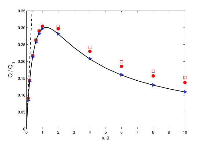
The integrals (25) and (26) were evaluated using the Matlab routine quadgk (MATLAB, 2010). represents the potential due to a thin charged disk, and decays exponentially at large distances, as does . The integration in (24) could therefore be truncated at a large value, taken to be (corresponding to a distance from the pore). To evaluate the second term in brackets in (24), the space was divided into sub–regions, with typically 500 intervals for and 200 for . Smaller intervals were used near the pore () and near the membrane (). For every pair , the integral was numerically evaluated and was obtained via trapezoidal summation within Matlab. Results are shown in Figure 2 with the asymptotic regime , described by (23), depicted by the dashed straight line of unit slope.
3 Flow through a hole in a membrane of finite thickness
In order to examine the validity of (24), the full Poisson-Nernst-Planck-Stokes system of equations was solved numerically using a finite volume method based on the open source CFD library OpenFOAM (OpenCFD, 2012). Our model has been described by Mao et al. (2013) and details of the implementation for the current problem are presented in the Appendix. The cases studied include membranes of thickness and in the regime of weak applied fields and low membrane charge. These conditions, stated in § 2.2, may be restated more conveniently as where and are dimensionless parameters characterizing the degree of membrane charge and the strength of the applied field respectively. In the simulations presented here, the values of these parameters were and so that (24) can be expected to be a reasonable approximation in the range .
The computed flow rate normalized by is shown by the symbols in Figure 2. Good agreement with (24) is obtained, but thicker membranes result in somewhat increased flow rates. The discrepancy increases at shorter Debye lengths.
The analysis of § 2 assumed that effects due to induced charge electroosmosis (ICEO) are negligible. However, Thamida & Chang (2002) have shown that ICEO generates vortices at sharp corners, and such vortices will inevitably be generated in the membrane geometry considered here. In the vicinity of the edge of the nanopore, where , the potential (19) on the membrane surface may be expanded as
| (28) |
If we assume that this potential is little modified when the membrane has a finite thickness , the potential gradient within the solid membrane due to the external potential is
| (29) |
and if the induced potential gradient normal to the surface within the liquid is . This corresponds to an induced surface charge (with accompanying charge cloud of couter-ions)
| (30) |
The analysis breaks down when where the detailed geometry near the edge of the pore becomes important. If the membrane has rounded edges, the curvature and the induced charge is at most . This may be neglected as long as it is small compared to , or equivalently, if . For common membrane materials (e.g. lipids and silica) , thus, as long as the applied field remains weak, ICEO effects are restricted to the neighbourhood of sharp corners.
The results of full numerical solutions of the Poisson-Nernst-Planck-Stokes equations reported in Figure 2 were computed with membrane permittivity . However, it is shown in the Appendix that numerical solutions for appropriate non-zero solid permittivities predict flow rates that differ little from those with in the parameter regime under consideration. The contribution of such effects to the net fluid flux, , is at best very weak. This is perhaps not surprising, since even when (as here) there are sharp corners, if the membrane is uncharged and the electrolyte is symmetric (with identical ionic mobilities), symmetry dictates that ICEO cannot generate a net flow through the pore. So although nonlinear effects such as ICEO can generate a net fluid flow through a charged membrane, the applied field must be larger than the fields considered here. An ICEO contribution to the fluid flux is in principle possible, but only for a charged membrane at high applied fields, as, for example, in the numerical results presented by Mao et al. (2013).
The reciprocal theorem used in § 2.2 enabled us to determine the volumetric flow rate through the pore without a full computation of the velocity field. This has the advantage of leading quickly to a value for . However, this approach hides other interesting features of the flow, such as eddies, whether generated by ICEO (Thamida & Chang, 2002) or by the pore throat restricting the flow (Park et al., 2006). These features are only revealed by full numerical computations, such as those discussed in the Appendix.
3.1 The limits of thick and thin membranes
Since the fluid flux through the pore is generated by the applied potential, , we can define an “electroosmotic conductance” in analogy to the electric conductance. If the membrane thickness , we have a long cylindrical pore with surface charge density at the wall. The electroosmotic flow velocity is then (Levine et al., 1975)
| (31) |
where is the equilibrium potential in the double layer, is the equilibrium potential at the wall, and . The equilibrium potential of a cylindrical pore in the Debye-Hückel limit is
| (32) |
Integrating the fluid velocity (31) over the cross-section we obtain the volumetric flow rate and hence the the electroosmotic conductance (Rice & Whitehead, 1965)
| (33) |
On the other hand, when the thickness , we expect the system to be identical to a hole in a zero–thickness membrane, and the electroosmotic conductance may be obtained using (24):
| (34) |
3.2 The electroosmotic access resistance of a nanopore
If a membrane of thickness containing a circular hole of radius separates two uniformly conducting regions, then the electrical resistance of the cylindrical hole increases, proportional to . This might suggest a vanishing resistance for an infinitely thin membrane. However, in reality, as the electrical resistance is dominated by entrance and exit effects, and can be determined from the electrical potential (19). This is called the “access resistance” of the pore and for a circular pore in an infinitely thin membrane it is described by a simple analytical formula (Hall, 1975).
An analogous situation applies to the problem of electroosmotic flow through a pore in a membrane. When the pore length is large compared to the pore radius , the flow conductance from (33) – a consequence of the fact that the electric field in the pore, . However, does not increase indefinitely as but instead approaches a finite value given by (34). The surface charge within the cylindrical pore goes to zero as . Electroosmotic motion is therefore determined by flow in the fluid on either side of the membrane, as described in § 2, and not by the cylindrical pore. Thus, in analogy to the corresponding electrical problem, may be regarded as an “access resistance” of the pore to electroosmotic flow.
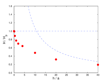
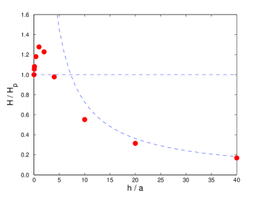
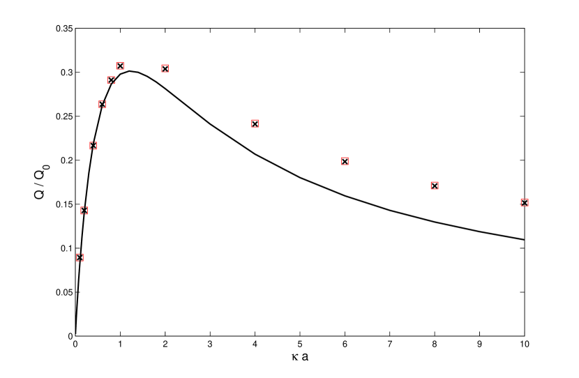
Figure 3 shows the electroosmotic conductance obtained from the finite volume numerical computations as a function of . The computed value of is normalized by obtained from (34). It is seen that approaches unity as and approaches for large . The dashed line representing was obtained from (33) and (34). The results of the full computations indicate that though does exhibit the expected limiting behaviors, it does not vary monotonically with at short Debye lengths. The origin of the peak at intermediate values of will be investigated further in future work.
4 Concluding Remarks
We have assumed that the surface charge density is sufficiently low that the zeta potential is small, at . Thus, the Poisson-Boltzmann equation can be linearized. Non-dimensional zeta potentials in colloidal systems, though not always small, are typically at most 5, and it is found that theories based on small potentials usually give useful qualitative insight into electrokinetic behaviour over this range of potentials (e.g. Levine et al. (1975)).
We have also assumed that the applied potential difference . Potential differences applied in experiments are typically of the same order as typical -potentials which in silica substrates vary in magnitude between and mV depending mainly on counter-ion concentration (Kirby & Hasselbrink, 2004a, b). For example, Keyser et al. (2006) describe experiments in which was in the range 30–100 mV. Nanopores (radius 5–10 nm) in graphene sheets have recently been used in DNA translocation experiments (Garaj et al., 2010; Schneider et al., 2010; Merchant et al., 2010). The applied voltage 0–200 mV in these experiments. The computations of Mao et al. (2013) predict that the electroosmotic flow rate through a pore in a membrane varies non-linearly with only at voltages greater than 100 mV. Thus, we again expect the results presented here to give at least a qualitative understanding of electroosmotic flow in such experiments.
Electroosmotic flow through nanopores has been shown to control the translocation velocity of charged polymers in resistive pulse experiments (Ghosal, 2006, 2007a). When the free translocation of the polymer is hindered by tethering it to a colloid held in an optical trap, the tethering force has been shown to be determined by the electroosmotic flow within the pore (Ghosal, 2007b; Keyser et al., 2006; Laohakunakorn et al., 2013a). Furthermore, it has been argued that the flow outside and in the vicinity of the nanopore controls the capture rate of polymers into the pore (Wong & Muthukumar, 2007), though the experimental evidence for this appears tentative at present.
In addition to the single molecule experiments mentioned above, our results should also be helpful in understanding the properties of nanoporous membranes that are used in batteries, water desalination and numerous other industrial applications. Gadaleta et al. (2014) have recently studied the electrical conductivity of a model membrane consisting of an array of nanopores. However, the applied voltage should also result in an electroosmotic flux, the calculation of which may be undertaken as a suitable generalization of the approach presented here. Since membrane bound organelles in cells contain nanopores that control the traffic of biological molecules across the membrane, our results may also be of interest in the biological context (see e.g. Gu et al. (2003)).
Acknowledgement
MM & SG acknowledge support from the NIH through Grant 4R01HG004842-03. SG was hosted by the Cavendish Laboratory, University of Cambridge, as visiting Professor with funds provided by the Leverhulme Trust. JDS thanks the Department of Applied Mathematics and Theoretical Physics, University of Cambridge, and the Institut de Mécanique des Fluides de Toulouse, for hospitality.
Appendix A Numerical solution of the PNP-Stokes equations
A.1 Numerical scheme
An electrohydrodynamic solver was developed to solve the Poisson–Nernst–Planck–Stokes (PNP–Stokes) system of equations using the finite volume method. The solver was based on the OpenFOAM CFD library (OpenCFD, 2012), a C++ library designed for computational mechanics, containing a collection of object–oriented classes developed to represent mesh, fields, matrices and the necessary operations on fields and tensors. It also provides functions to handle finite volume discretization and matrix equation solving.
The time–independent PNP–Stokes equations are:
| (35) | |||||
| (36) | |||||
| (37) | |||||
| (38) |
In our simulation we consider a 1–1 symmetric electrolyte solution containing ions with equal mobilities. The boundary conditions to be satisfied by the solution are discussed in § A.2.
We apply the following scheme to solve the PNP–Stokes equations. We start from a zero flow field. Equations (35) and (36) are solved sequentially in a loop with under-relaxation until the absolute residual is smaller than . Under–relaxation is necessary because the PNP system is non–linear. The electric volume force is obtained from this solution and used explicitly in the next step: the solution of the incompressible Stokes flow: (37) and (38). The SIMPLE algorithm is used with a fixed volume force density. The flow field is then substituted into (36). The PNP equations are then solved again using the updated flow field. An outer loop is constructed to iterate over the PNP loop and Stokes flow module.
For the finite volume discretization of the governing equations, central differences are used for all diffusive terms in (36) and viscous terms in (37). A second–order upwind scheme is used for the convective terms in (36). The discretized linear system is solved using a pre-conditioned conjugate gradient solver if the matrix is symmetric or a pre-conditioned bi–conjugate gradient solver if the matrix is asymmetric. The details of the numerical algorithm are given by Ferziger & Perić (2002).
A.2 Mathematical model of the nanopore
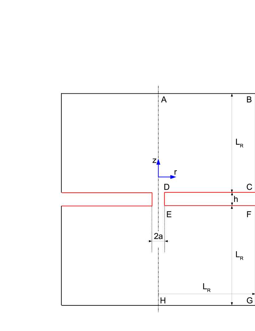
A schematic view of the axisymmetric geometry used for the full numerical simulations is provided in Figure 4. It consists of a circular hole of radius in a solid dielectric membrane CDEF of arbitrary thickness . The membrane surfaces CD, DE and EF have a uniform surface charge density . Two large cylindrical reservoirs are connected to the pore, one at each end. The length and radius of both the reservoirs are identical, and are , chosen to be much larger than either the hole radius or the Debye length in order to approximate an infinite reservoir.
We adopt the following boundary conditions (Mao et al., 2013). The ion number densities on AB and GH are constant, and equal to the number density in the bulk solution far from any charged surfaces. The electrical potentials are uniform on AB and on GH, with a potential difference of between the top (AB) and bottom (GH). The pressure on AB is uniform and equal to that on GH. On the side walls BC and FG, the radial electric field, ionic flux and radial velocity, which decay away from the pore, are set to zero. A zero tangential shear stress is imposed on flow parallel to the side walls. At the membrane surfaces CD, DE and EF, a no–flux condition is used for (36), a no–slip condition for the flow; the electric field undergoes a jump across the solid-fluid interface such that where is the electrical permittivity of the fluid and is the permittivity of the membrane, is the electric field at the interface within the membrane and is the unit normal at the surface directed into the fluid. The potential is continuous across the interface.
The strength of the applied field and the amount of surface charge can be characterized by the dimensionless parameters and respectively. In the simulations presented here, the values of these parameters were kept fixed at and . The flow rate was obtained by numerically integrating the –component of the velocity over the plane .
A.3 Effect of membrane polarizability
If the membrane polarizability is sufficiently small that , then the jump condition of the normal component of the field may be replaced by . In this case, the computational domain may be restricted to include only the fluid phase. This approximation was adopted for the results presented in Figures 2 and 3. Thus, effects due to Induced Charge Electroosmosis (ICEO) were neglected. The results of a calculation to test the validity of this assumption in the parameter range of interest are shown in Figure 5. The data from Figure 2 for a non-polarizable membrane of thickness are reproduced in Figure 5. For comparison, the result of a second calculation in which the dielectric constant of the membrane material was set to (corresponding to silica) is also shown. The electrolyte is considered polarizable with a dielectric constant of . It is seen that the effect of membrane polarizability on the flow rate is negligible.
References
- Alberts et al. (1994) Alberts, B., Bray, D., Lewis, J., Raff, M., Roberts, K. & Watson, J.D. 1994 Molecular Biology of the Cell. New York: Garland Publishing, Taylor & Francis Group.
- Chang & Yossifon (2009) Chang, H.C. & Yossifon, G. 2009 Understanding electrokinetics at the nanoscale: A perspective. Biomicrofluidics 3 (1), 012001 (15pp).
- Chang et al. (2012) Chang, H.C., Yossifon, G. & Demekhin, E. A. 2012 Nanoscale electrokinetics and microvortices: How microhydrodynamics affects nanofluidic ion flux. Annual Review of Fluid Mechanics 44 (1), 401–426.
- van Dorp et al. (2009) van Dorp, S., Keyser, U. F., Dekker, N. H., Dekker, C. & Lemay, S. 2009 Origin of the electrophoretic force on DNA in solid-state nanopores. Nature Physics 5 (5), 347–351.
- Ferziger & Perić (2002) Ferziger, J. H. & Perić, M. 2002 Computational Methods for Fluid Dynamics. Berlin, Heidelberg, New York: Springer-Verlag.
- Gadaleta et al. (2014) Gadaleta, A., Sempere, C., Gravelle, S., Siria, A., Fulcrand, R., Ybert, C. & Bocquet, L. 2014 Sub-additive ionic transport across arrays of solid-state nanopores. Physics of Fluids 26 (1), 012005.
- Garaj et al. (2010) Garaj, S., Hubbard, W., Reina, A., Kong, J., Branton, D. & Golovchenko, J. 2010 Graphene as a subnanometre trans-electrode membrane. Nature 467 (7312), 190–193.
- Ghosal (2006) Ghosal, S. 2006 Electrophoresis of a polyelectrolyte through a nanopore. Physical Review E 74 (4), 041901 (5pp).
- Ghosal (2007a) Ghosal, S. 2007a Effect of salt concentration on the electrophoretic speed of a polyelectrolyte through a nanopore. Physical Review Letters 98 (23), 238104 (4pp).
- Ghosal (2007b) Ghosal, S. 2007b Electrokinetic-flow-induced viscous drag on a tethered DNA inside a nanopore. Physical Review E 76 (6), 061916 (3pp).
- Gu et al. (2003) Gu, L., Cheley, S. & Bayley, H. 2003 Electroosmotic enhancement of the binding of a neutral molecule to a transmembrane pore. Proceedings of the National Academy of Sciences of the United States of America 100 (26), 15498–15503.
- Hall et al. (2010) Hall, A. R., Scott, A., Rotem, D., Mehta, K., Bayley, H. & Dekker, C. 2010 Hybrid pore formation by directed insertion of -haemolysin into solid-state nanopores. Nature Nanotechnology 5 (12), 874–877.
- Hall (1975) Hall, J. E. 1975 Access resistance of a small circular pore. The Journal of General Physiology 66, 531–532.
- Happel & Brenner (1983) Happel, J. & Brenner, H. 1983 Low Reynolds number hydrodynamics: with special applications to particulate media. The Hague: Martinus Nijhoff Publishing.
- Henry (1931) Henry, D.C. 1931 The cataphoresis of suspended particles. Part 1. the equation of cataphoresis. Proceedings of the Royal Society A 133 (821), 106–129.
- Hu et al. (2012) Hu, G., Mao, M. & Ghosal, S. 2012 Ion transport through a graphene nanopore. Nanotechnology 23 (39), 395501 (8pp).
- Kasianowicz et al. (1996) Kasianowicz, J. J., Brandin, E., Branton, D. & Deamer, D. W. 1996 Characterization of individual polynucleotide molecules using a membrane channel. Proceedings of the National Academy of Sciences of the United States of America 93 (24), 13770–13773.
- Keyser et al. (2006) Keyser, U. F., Koeleman, B. N., van Dorp, S., Krapf, D., Smeets, R., Lemay, S., Dekker, N. & Dekker, C. 2006 Direct force measurements on DNA in a solid-state nanopore. Nature Physics 2 (7), 473–477.
- Kirby & Hasselbrink (2004a) Kirby, B.J. & Hasselbrink, E.F. 2004a Zeta potential of microfluidic substrates: 1. theory, experimental techniques, and effects on separations. Electrophoresis 25, 187–202.
- Kirby & Hasselbrink (2004b) Kirby, B.J. & Hasselbrink, E.F. 2004b Zeta potential of microfluidic substrates: 2. data for polymers. Electrophoresis 25, 203–213.
- Künkele et al. (1998) Künkele, K. P., Heins, S. & Dembowski, M. 1998 The preprotein translocation channel of the outer membrane of mitochondria. Cell 93, 1009–1019.
- Laohakunakorn et al. (2013a) Laohakunakorn, N., Ghosal, S., Otto, O., Misiunas, K. & Keyser, U.F. 2013a DNA interactions in crowded nanopores. Nano Letters 13 (6), 2798–2802.
- Laohakunakorn et al. (2013b) Laohakunakorn, N., Gollnick, B., Moreno-Herrero, F., Aarts, D., Dullens, R., Ghosal, S. & Keyser, U. F. 2013b A landau–squire nanojet. Nano Letters 13 (11), 5141–5146.
- Levine et al. (1975) Levine, S., Marriott, J.R, Neale, G. & Epstein, N. 1975 Theory of electrokinetic flow in fine cylindrical capillaries at high zeta-potentials. Journal of Colloid and Interface Science 52 (1), 136–149.
- Li et al. (2003) Li, J., Gershow, M., Stein, D., Brandin, E. & Golovchenko, J. 2003 DNA molecules and configurations in a solid-state nanopore microscope. Nature Materials 2 (9), 611–615.
- Mao et al. (2013) Mao, M., Ghosal, S. & Hu, G. 2013 Hydrodynamic flow in the vicinity of a nanopore induced by an applied voltage. Nanotechnology 24 (24), 245202 (10pp).
- Martin et al. (1991) Martin, J., Mahlke, K. & Pfanner, N. 1991 Role of an energized inner membrane in mitochondrial protein import: drives the movement of presequences. Journal of Biological Chemistry 266, 18051–18057.
- MATLAB (2010) MATLAB 2010 version 7.10.0 (R2010a). Natick, Massachusetts: The MathWorks Inc.
- Matouschek et al. (2000) Matouschek, A., Pfanner, N. & Voos, W. 2000 Protein unfolding by mitochondria: The hsp70 import motor. EMBO Reports 1, 404–410.
- Merchant et al. (2010) Merchant, C., Healy, K., Wanunu, M., Ray, V., Peterman, N., Bartel, J., Fischbein, M., Venta, K., Luo, Z., Johnson, A., & Drndić, M. 2010 DNA translocation through graphene nanopores. Nano Letters 10 (8), 2915–2921.
- Morse & Feshbach (1953) Morse, P. & Feshbach, H. 1953 Methods of Theoretical Physics. New York: McGraw-Hill.
- Murtsovkin (1996) Murtsovkin, V. A. 1996 Nonlinear flows near polarized disperse particles. Colloid Journal 58, 341–349.
- OpenCFD (2012) OpenCFD 2012 OpenFOAM - The Open Source CFD Toolbox - User’s Guide, 2nd edn. OpenCFD Ltd., United Kingdom.
- Park et al. (2006) Park, S. Y., Russo, C. J., Branton, D. & Stone, H. A. 2006 Eddies in a bottleneck: An arbitrary Debye length theory for capillary electroosmosis. Journal of Colloid and Interface Science 297 (2), 832–839.
- Pfanner & Neupert (1990) Pfanner, N. & Neupert, W. 1990 The mitochondrial protein import apparatus. Annual Review of Biochemistry 59, 331–353.
- Rice & Whitehead (1965) Rice, C.L. & Whitehead, R. 1965 Electrokinetic flow in a narrow cylindrical capillary. The Journal of Physical Chemistry 69, 4017–4024.
- Rubinstein & Shtilman (1979) Rubinstein, I. & Shtilman, L. 1979 Voltage against current curves of cation exchange membranes. Journal of the Chemical Society, Faraday Transactions 2: Molecular and Chemical Physics 75, 231–246.
- Saville (1977) Saville, D.A. 1977 Electrokinetic effects with small particles. Annual Review of Fluid Mechanics 9, 321–337.
- Schneider et al. (2010) Schneider, G. F, Kowalczyk, S., Calado, V., Pandraud, G., Zandbergen, H., Vandersypen, L. & Dekker, C. 2010 DNA translocation through graphene nanopores. Nano Letters 10 (8), 3163–3167.
- Sherwood & Stone (1995) Sherwood, J. D. & Stone, H. A. 1995 Electrophoresis of a thin charged disk. Physics of Fluids 7 (4), 697–705.
- Siwy (2006) Siwy, Z. S. 2006 Ion-current rectification in nanopores and nanotubes with broken symmetry. Advanced Functional Materials 16 (6), 735–746.
- Siwy & Fulinsski (2004) Siwy, Z. S. & Fulinsski, A. 2004 A nanodevice for rectification and pumping ions. American Journal of Physics 72 (5), 567–574.
- Smeets et al. (2006) Smeets, R. M. M., Keyser, U. F., Krapf, D., Wu, M. Y., Dekker, N. H. & Dekker, C. 2006 Salt dependence of ion transport and DNA translocation through solid-state nanopores. Nano Letters 6 (1), 89–95.
- Squires & Bazant (2004) Squires, T. M. & Bazant, M. Z. 2004 Induced-charge electro-osmosis. Journal of Fluid Mechanics 509, 217–252.
- Storm et al. (2005a) Storm, A. J., Chen, J. H., Zandbergen, H. W. & Dekker, C. 2005a Translocation of double-strand DNA through a silicon oxide nanopore. Physical Review E 71 (5), 051903 (10pp).
- Storm et al. (2005b) Storm, A. J., Storm, C., Chen, J. H., Zandbergen, H., Joanny, J. F. & Dekker, C. 2005b Fast DNA translocation through a solid-state nanopore. Nano Letters 5 (7), 1193–1197.
- Thamida & Chang (2002) Thamida, S. K. & Chang, H. C. 2002 Nonlinear electrokinetic ejection and entrainment due to polarization at nearly insulated wedges. Physics of Fluids 14 (12), 4315–4328.
- Vlassiouk & Siwy (2007) Vlassiouk, I. & Siwy, Z. S. 2007 Nanofluidic diode. Nano Letters 7 (3), 552–556.
- Vlassiouk et al. (2008a) Vlassiouk, I., Smirnov, S. & Siwy, Z. 2008a Nanofluidic ionic diodes. comparison of analytical and numerical solutions. ACS Nano 2 (8), 1589–1602.
- Vlassiouk et al. (2008b) Vlassiouk, I., Smirnov, S. & Siwy, Z. S. 2008b Ionic selectivity of single nanochannels. Nano Letters 8 (7), 1978–1985.
- Wong & Muthukumar (2007) Wong, C. T. A. & Muthukumar, M. 2007 Polymer capture by electro-osmotic flow of oppositely charged nanopores. The Journal of Chemical Physics 126 (16), 164903 (5pp).
- Yossifon & Chang (2008) Yossifon, G. & Chang, H. C. 2008 Selection of nonequilibrium overlimiting currents: Universal depletion layer formation dynamics and vortex instability. Physical Review Letters 101 (25), 254501 (4pp).
- Zaltzman & Rubinstein (2007) Zaltzman, B. & Rubinstein, I. 2007 Electro-osmotic slip and electroconvective instability. Journal of Fluid Mechanics 579, 173–226.