EFTCAMB/EFTCosmoMC: Numerical Notes v3.0
Abstract
EFTCAMB/EFTCosmoMC are publicly available patches to the CAMB/CosmoMC codes implementing the effective field theory approach to single scalar field dark energy and modified gravity models. With the present numerical notes we provide a guide to the technical details of the code. Moreover we reproduce, as they appear in the code, the complete set of the modified equations and the expressions for all the other relevant quantities used to construct these patches. We submit these notes to the arXiv to grant full and permanent access to this material which provides very useful guidance to the numerical implementation of the EFT framework. We will update this set of notes when relevant modifications to the EFTCAMB/EFTCosmoMC codes will be released.
The present version is based on the version of EFTCAMB/EFTCosmoMCSep17.
pacs:
98.80I Introduction
In the quest to address one of the most pressing problems of modern cosmology, i.e. cosmic acceleration, an effective field theory approach has been recently proposed Gubitosi:2012hu ; Bloomfield:2012ff . The virtue of this approach relies in the model-independent description of this phenomenon as well as in the possibility to cast into the EFT language most of the single field DE/MG gravity models of cosmological interest Gubitosi:2012hu ; Bloomfield:2012ff ; Gleyzes:2013ooa ; Bloomfield:2013efa . The EFT action is written in unitary gauge and Jordan frame and it contains all the operators invariant under time-dependent spatial diffeomorphisms, ordered in power of perturbations and derivatives. These operators enter in the action with a time dependent function in front of them, to which we will refer to as EFT functions. The DE/MG models encoded in this formalism have one extra scalar d.o.f. and a well defined Jordan frame; in unitary gauge the scalar field is hidden in the metric. In order to study the
dynamics of scalar perturbations, it is better to make its dynamics manifest via the Stckelberg technique, i.e. restoring the time diffeomorphism invariance through an infinitesimal time coordinate transformation. Then a new scalar field appears in the action, the so called Stckelberg field.
The EFT action in conformal time reads
| (1) |
where is the Planck mass, overdots represent derivatives with respect to conformal time and indicates three dimensional spatial derivatives. ,, are the only three EFT functions describing the background dynamics, hence the name background functions. While the dynamics of linear scalar perturbations is described by the second order EFT functions, , in combination with the background ones. We parametrize the conformal coupling to gravity via the function instead of Gubitosi:2012hu ; Bloomfield:2012ff for reasons of numerical accuracy. Finally, is the action for all matter fields, . The EFT approach relies on the assumption of the validity of the weak equivalence principle which ensures the existence of a metric universally coupled to matter fields and therefore of a well defined Jordan frame.
In Hu:2013twa ; Raveri:2014cka , we introduced EFTCAMB which is a patch of the publicly available Einstein-Boltzmann solver, CAMB CAMB ; Lewis:1999bs . The code implements the EFT approach, allowing to study the linear cosmological perturbations in a model-independent framework via the pure EFT procedure, although it ensures to investigate the dynamics of linear perturbations of specific single scalar field DE/MG models via the mapping EFT procedure, once the matching is worked out. EFTCAMB evolves the full perturbation equations on all linear scales without relying on any quasi static approximation. Moreover it checks the stability conditions of perturbations in the dark sector in order to ensure that the underlying gravitational theory is acceptable. Finally, it enables to specify the expansion history by choosing a DE equation of state among several common parametrizations, allowing phantom-divide crossings. To interface EFTCAMB with cosmological observations we equipped it with a modified version of CosmoMC Lewis:2002ah , what we dub EFTCosmoMC Raveri:2014cka . EFTCosmoMC allows to practically perform tests of gravity and get constraints on the parameter space using cosmological data sets. The stability conditions implemented in EFTCAMB translate into EFTCosmoMC as viability priors to impose on parameters describing the dark sector. The first release of the code includes data such as Planck, WP, BAO and Planck lensing. The present version is fully compatible with all data sets available in CosmoMC. The EFTCAMB/EFTCosmoMC package is now publicly available for download at http://www.eftcamb.org.
After EFTCAMB some other general purpose Einstein-Boltzmann codes modeling scalar-tensor theories have been developed, such as hi-class Zumalacarregui:2016pph and COOP Huang:2015srv . In a recent paper Bellini:2017avd it has been shown that EFTCAMB (Sep17) and hi-class agree to a high level of accuracy, while their agreement with COOP is sufficiently high only on large scales. It has been also shown that the implementation of the low-energy Hořava gravity model in EFTCAMB gives the same results of the LVDM CLASS code Blas:2012vn .
Throughout this Numerical Notes we will always use the following conventions:
-
•
The overdot represents derivation with respect to conformal time while the prime represents derivation with respect to the scale factor , unless otherwise specified.
-
•
In what follows we define a new dimensionless Stckelberg field: , i.e. the -field in the action (I) multiplied by and divided by . For the rest of the notes we will suppress the tilde to simplify the equations so is written as , if there is no confusion.
-
•
We redefine all the second order EFT functions to make them dimensionless and to facilitate their inclusion in the code:
(2) Let us notice that after v2.0 we have slightly changed the definition of the second order EFT functions w.r.t. the convention used in v1.0 and v1.1. These new definitions do not change the general structure and physics in the code, but they allow for a more direct and cleaner implementation of Horndeski models Horndeski:1974wa ; Deffayet:2009mn . For the sake of clarity let us list the explicit correspondence between this new convention and that one used in the previous releases (v1.0 and v1.1), in terms of the ’s:
(3) -
•
We define all the EFT functions , c, and the -functions as function of the scale factor .
II The structure of the code
The structure of the EFTCAMB code is illustrated in the flowchart of Figure 1. There is a number associated to each model selection flag; such number is reported in Figure 1 and it controls the behaviour of the code. The main code flag is EFTflag, which is the starting point after which all the other sub-flags, can be chosen according to the user interests.
-
•
The number corresponds to the standard CAMB code. Every EFT modification to the code is automatically excluded by this choice.
-
•
The number corresponds to pure EFT models. The PureEFTmodel flag controls which basis for pure EFT to use. For the choice the user needs to select a model for the background expansion history via the EFTwDE flag. Various common parametrizations for the DE equation of state are natively included in the code. The implementation details of the dark energy equations of state can be found in Section IV.2.1. Finally, to fully specify the pure EFT model, one has to fix the EFT functions behaviour as functions of the scale factor . The corresponding flags for the model selection are: PureEFTmodelOmega for the model selection of the EFT function and PureEFTmodelGammai, with for the EFT functions. Some built-in models are already present in the code and can be selected with the corresponding number, see Flowchart 1. The details about these models can be found in Section V. There is also the possibility to use the flag PureEFTHorndeski to restrict pure EFT models to Horndeski one. The code will then internally set the behaviour of the EFT functions , , according to eq. (54) in order to cancel high order derivatives, at this point choices made for these functions will be ignored (see Section V.1 for more details). After setting these flags the user has to define the values of the EFT model parameters for the chosen model. Every other value of parameter and flag which do not concern the chosen model is automatically ignored.
-
•
The number corresponds to the implementation of alternative model-independent parametrizations in terms of EFT functions. A lot of alternative parametrizations already present in literature can be completely described by using the versatility of the EFT approach allowing to preserve all the advantages of EFTCAMB. An alternative parametrization can be chosen by changing the flag AltParEFTmodel. See Section VI for details.
-
•
The number corresponds to the designer mapping EFT procedure. Also in this case the EFTwDE flag controls the background expansion history which works as in the previous case
For the mapping case the user can investigate a particular DE/MG model once the matching with the EFT functions is provided and the background evolution has been implemented in the EFT code.
The model selection flag for the mapping EFT procedure is DesignerEFTmodel.
Various models are already included in the code and their implementation details are presented in Section VII.
•
The number corresponds to the full mapping EFT procedure. In this case the background expansion history is not set by a choice of and a model has to be fully specified. The code will then solve the background equations for the given model to map it into the EFT framework. Low energy Hořava gravity has been included as the first example of the implementation of full mapping models. More models will be gradually filled in the near future. See Section VIII for details.
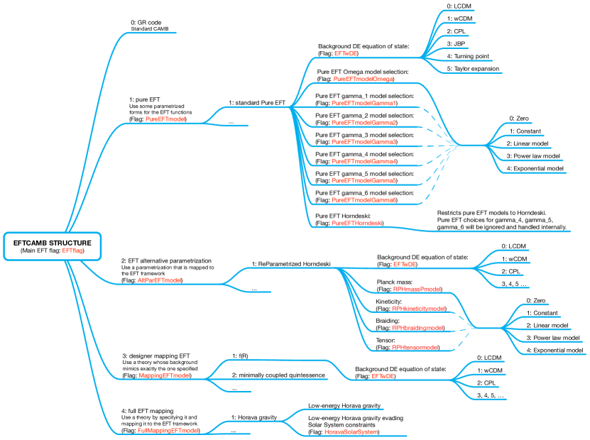 Figure 1: Flowchart of the structure of EFTCAMB: blue lines correspond to flags that are already present in the code.
In addition EFTCAMB takes advantage of the feedback mechanism of CAMB with the following modifications:
•
feedback level=0 no feedback from EFTCAMB nor from EFTCosmoMC;
•
feedback level=1 basic feedback, no feedback from EFTCAMB when called from EFTCosmoMC;
•
feedback level=2 advanced feedback, no feedback from EFTCAMB when called from EFTCosmoMC;
•
feedback level=3 debug feedback also when EFTCAMB is called from EFTCosmoMC;
Figure 1: Flowchart of the structure of EFTCAMB: blue lines correspond to flags that are already present in the code.
In addition EFTCAMB takes advantage of the feedback mechanism of CAMB with the following modifications:
•
feedback level=0 no feedback from EFTCAMB nor from EFTCosmoMC;
•
feedback level=1 basic feedback, no feedback from EFTCAMB when called from EFTCosmoMC;
•
feedback level=2 advanced feedback, no feedback from EFTCAMB when called from EFTCosmoMC;
•
feedback level=3 debug feedback also when EFTCAMB is called from EFTCosmoMC;
III The structure of the modification
In order to implement the EFT formalism in the CAMB and CosmoMC codes we had to modify several files. The complete, automatic, code documentation is available at https://eftcamb.github.io/EFTCAMB/. To further help the user in understanding our part of code and/or applying the EFT modification to an already modified version of CAMB/CosmoMC we enclosed every modification that we made inside the following commented code lines:
! EFTCAMB MOD START
...
! EFTCAMB MOD END
for the CAMB part and:
! EFTCOSMOMC MOD START
...
! EFTCOSMOMC MOD END
for the CosmoMC part.
We also provide a developers version of the code at https://github.com/EFTCAMB/EFTCAMB. The tools provided by Github to visualize the history of the modifications of the code will, from now on, supersede the guides to the EFTCAMB/EFTCosmoMC modifications.
The step by step guide to the EFTCAMB modification v1.0 and v1.1 and v.2.0 will still be available at http://www.eftcamb.org/codes/guide_EFTCAMB.html and the EFTCosmoMC one at http://www.eftcamb.org/codes/guide_EFTCosmoMC.html.
IV Implementation of the modified equations
The implementation of the background in the code is described at length in Hu:2013twa . Here we shall review some of the more technical aspects and reproduce the equations in the form in which they enter the code.
IV.1 General EFT Background
Starting from the general expressions for the cosmological background in EFT we can write the expansion history as a function of the EFT functions directly. This results in:
| (4) |
IV.2 Designer Background
Given the high degree of freedom already at the level of background, and since the focus will be on the dynamics of linear perturbations, it is common to adopt a designer approach as described in Gubitosi:2012hu ; Bloomfield:2012ff . First of all one writes the background equations as follows:
| (5) |
where the prime stands for derivative w.r.t. the scale factor , are the energy density and pressure of matter (e.g. dark matter, radiation and massless neutrinos) and encode the contributions from the extra scalar field into the form of an energy density and pressure of dark energy. For the matter components, one has the following continuity equations, and corresponding solutions:
| (6) |
where is the energy density parameter today, respectively of matter sector and dark energy, and is the present time Hubble parameter. Finally, are the density and pressure contributions due to massive neutrinos. The equation of state of massive neutrinos has a complicated, time dependent expression, hence the code computes directly . As the treatment of massive neutrinos in EFTCAMB is exactly the same as CAMB we refer the user to Ma:1995ey ; cambnotes . However, let us stress that in EFTCAMB the indirect interaction (via gravity) of massive neutrino and DE/MG sectors has been consistently taken into account both at the background and perturbations level, see also Hu:2014sea . With this setup, a background is fixed specifying . We illustrate in the next Section IV.2.1 the models that are currently implemented in the code. After the expansion history has been chosen one can then determine in terms of and ; namely, combining eq. (5) and eq. (6) with the EFT background eqs. (12,13) in Hu:2013twa one has:
| (7) | |||||
| (8) | |||||
| (9) | |||||
| (10) | |||||
As discussed in the Sections V and VII, depending on whether one wants to implement a pure or mapping EFT model, the choice for changes. After fixing the expansion history, in the former case one selects an anstz for , while in the latter case one determines via the matching the corresponding to the chosen model. In this case one has to separately solve the background equations for the given model, which might be done with a model-specific designer approach. In fact, this is the methodology we adopt for models (see Section VII.1).
IV.2.1 Effective Dark Energy equation of state parametrizations
Several models for the background expansion history have been implemented in the code:
-
- The CDM expansion history:
(11) -
- The CDM model:
(12) In code notation: .
-
- The CPL parametrization Chevallier:2000qy ; Linder:2002et :
(13) where and are constant and indicate, respectively, the value and the derivative of today.
In code notation: and . - The generalized Jassal-Bagla-Padmanabhan parametrization Jassal:2004ej ; Jassal:2006gf : (14) where is the value of for and , while encodes the time of maximum deviation from and the extent of this deviation. For this reduces to the usual CPL parametrization. In code notation: , and . - The turning point parametrization Hu:2014ega : (15) here is where is the value of the scale factor at the turning point, and is its time derivative. In code notation: , and . - The Taylor expansion around : (16) where and are respectively the 2nd and 3rd time derivatives of . In code notation: , , and . - User defined: the EFTCAMB code includes the possibility for the user to define his/her own DE equation of state parametrization and it will properly account for it in any calculation. Let us notice that this option can be safely chosen without any modification in the structure of the code if the parametrized form of is given as a function of the scale factor . These definitions of are shared by the pure EFT and designer EFT modules and can be consistently used for both choices of model.
IV.3 Other Background Quantities
Finally, for the purposes of the code, it is useful to compute the following EFT dark fluid components that can be derived from eq. (10) of Hu:2013twa :
| (17) | |||||
| (18) | |||||
| (19) | |||||
| (20) |
IV.4 Linear Scalar Perturbations in EFT: code notation
In this Section we write the relevant equations that EFTCAMB uses Ma:1995ey . We write them in a compact notation that almost preserves the form of the standard equations simplifying both the comparison with the GR limit and the implementation in the code. The dynamical equations that EFTCAMB evolves can be written111Notice that working in the Jordan frame ensures that the energy-momentum conservation equations will not change with respect to their GR form. For this reason the evolution equations for density and velocity are not reported here. as:
| (21) | |||
| (22) |
while constraint equations take the form:
| (23) | ||||
| (24) | ||||
| (25) | ||||
| (26) | ||||
| (27) |
where and are the standard CAMB variables. In these expressions we wrote the same prefactor, , in eqs. (23) and (24), and , in eqs. (23) and (27), but we have to stress that they might be different if other second order EFT operators are considered. In addition the last expression (27) has two forms: the first is the standard one while the second one is used when the CAMB code uses the RSA approximation. At last, to compute the observable spectra we had to define two auxiliary quantities:
| (28) | ||||
| (29) |
The coefficients for the field equation, once a complete de-mixing is achieved, can not be divided into contributions due to one operator at a time so we write here their full form:
| (30) | ||||
| (31) | ||||
| (32) |
On the other hand the non-zero contributions to be added to the Einstein equations can be written for each operator separately and are listed in the following as respectively. We adopt the following convention: and the same applies to all the other terms.
-
Background operators
| (33) | |||||
:
| (34) |
:
| (35) |
:
| (36) |
:
| (37) | |||||
:
| (38) |
:
| (39) |
IV.5 Linear Tensor Perturbations in EFT: code notation
The tensor component of the B-mode polarization of the CMB can be used to further constrain modifications of gravity Amendola:2014wma ; Raveri:2014eea . In this Section we write the relevant equation that EFTCAMB uses to build the tensor component of the CMB spectra. Since we are working in the Jordan frame only the propagation equation for tensor perturbations needs to be modified into:
| (40) |
where:
| (41) |
and contains the neutrinos and photons contribution to the tensor component of anisotropic stress.
IV.6 Viability conditions
In this Section we list the viability priors that EFTCAMB naturally enforces on the EFT functions in order to ensure that the theory under consideration is stable. We separate these conditions in a set of physical ones and a set of mathematical ones, as described in the following. The full set of physical conditions for the general EFT action is a very complex matter that is the focus of our ongoing work. Here we report a preliminary version of them that contains the ghost and gradient stability for the subset of the EFT corresponding to GLPV theories Gleyzes:2014dya , for which the mixing between the matter and gravity perturbations has been considered Kase:2014cwa . The full class of Horndeski models is included in these theories. Specifically, when and (i.e. we consider GLPV theories) the kinetic and gradient stability conditions reduce respectively to
| (42) | |||
| (43) |
where
| (44) | |||
| (45) | |||
| (46) | |||
| (47) | |||
| (48) | |||
| (49) | |||
| (50) | |||
| (51) |
Let us notice that for models characterized by and/or the stability conditions need to be derived separately; while, the full set of perturbative equations evolved by EFTCAMB is still valid and can be used for a thorough investigation of linear perturbations, the derivation of the corresponding stability conditions is work in progress. Therefore, for these cases the user has to be careful in setting appropriate stability conditions for the chosen model. Hořava gravity belongs to this class of theories and in the current version of the code we implement specific stability conditions as explained in Section VIII.1.
Along with the physical stability conditions discussed above, and that are work in progress, we have a set of mathematical stability conditions which guarantee that the perturbations in the dark sector are stable. They are turn off by default, but can be turned on by the user providing a second layer of protection from unhealthy models. They are imposed via the equation and we call them mathematical (or classical) stability conditions. Rewriting the field equation as follows:
| (52) |
the conditions that we impose read:
-
•
: well defined field equation;
-
•
No fast exponential growing of field perturbations:
then – if then • : well defined tensor perturbations equation;
Let us notice that all the conditions based on scale dependent relations are enforced from up to , where is the maximum wavenumber that CAMB evolves.
The EFTCAMB code allows the user to have full control over the prior that are enforced by means of a set of flags contained in the parameter file paramsEFT.ini that will do the following:
-
•
EFTmathematicalstability: decides whether to enforce requirements of mathematical stability;
-
•
EFTphysicalstability: establishes whether to use physical viability conditions;
-
•
EFTadditionalpriors: determines whether to use model specific priors on cosmological parameters;
IV.7 Initial Conditions
We assume that DE perturbations are sourced by matter perturbations at a sufficiently early time so that the theory is close to GR and initial conditions can be taken to be:
| (53) |
where is the time at which the code is switching from GR to DE/MG. This scheme is enforced here to speed up models that are too close to GR at early times.
Studying early DE/MG models requires the user to modify the parameter flag EFTturnonpiInitial to a suitable value. Its default value is set to be EFTturnonpiInitial=0.01. The initial conditions for matter components and curvature perturbations are set in the radiation dominated epoch ().
V Pure EFT models
In the pure EFT procedure once the background expansion history has been fixed, one has to specify the functional forms for the EFT functions. EFTCAMB allows to choose among several models. We write them here just for but the same time dependence can be assumed for any other EFT function .
-
Constant models: ;
-
Linear models: ;
-
Power law models: ;
-
Exponential models: .
The first option includes the minimal coupling, corresponding to ; the linear model can be thought of as a first order approximation of a Taylor expansion; while the power law is inspired by . There is also the possibility for the user to choose an arbitrary form of according to any anstz the user wants to investigate, defining them as a function of the scale factor and by specifying their derivatives with respect to the scale factor. Of course the possibility to set all/some second order EFT functions to zero is included.
In the code we implemented a slot for user defined forms which can be easily spotted inside the file EFT_main.f90.
Once the user defined form has been specified no other modifications to the code are required but numerical stability is not guaranteed.
Notice also that due to the structure of our modification it is possible to use, inside the definition of the EFT functions, cosmological parameters like and .
Code notation for pure EFT models:
-
•
, ;
-
•
, ;
-
•
, ;
-
•
, ;
-
•
, ;
-
•
, ;
-
•
, .
V.1 Horndeski implementation into EFTCAMB
The Horndeski gravity Horndeski:1974wa or Generalized Galileons (GG) Deffayet:2009mn correspond to the most general scalar tensor theory with second order derivatives in the equations. As discussed in Gleyzes:2013ooa ; Bloomfield:2013efa they are a subset of the models encompassed by the EFT framework which corresponds to the following conditions on the EFT functions (in terms of our convention):
| (54) |
Models belonging to this class can be implemented into EFTCAMB following three different procedures as we discuss in what follows.
-
•
Pure EFT: if one is interested in investigating the general Horndeski class, rather than implementing a specific model within it, then one can opt to work directly with the four EFT functions that describe the Horndeski class in the EFT framework Bloomfield:2013efa , i.e. , after an expansion history has been chosen (). In this case one has to parametrize the dependence of the EFT functions on time instead of specifying the functions (). The limit of this procedure is that the user loses information about the corresponding theory as an inverse machinery to reconstruct the Horndeski functions is not possible to implement.
-
•
EFT implementation of the parametrization proposed in Bellini:2014fua ; the latter is a parametrization of Horndeski theory in terms of five functions of time which are chosen to correspond to specific physical properties of the scalar d.o.f.. Let us notice that it is equivalent to the pure EFT approach, and hence it shares the same limit mentioned above, while perhaps being closer to the phenomenology and the observables in the specific choice of the five functions. See Section VI.1 for details.
-
•
Full/designer Mapping approaches: one starts from a specific Horndeski/GG model, i.e. from a choice of the 4 unknown functions (where and ) and in the case of designer mapping by specifying also the expansion history, i.e. ; proceeds solving the background field equations for this model and then, through the mapping described in Gleyzes:2013ooa ; Bloomfield:2013efa , reconstructs the corresponding EFT functions. At this point EFTCAMB has all the ingredients to evolve linear perturbations. This approach emphasizes the choice of a specific theory and its implementation in EFTCAMB is work in progress.
Here we will focus on the pure EFT approach leaving the other options to the specific Sections. To use the code using the EFT approach restricted to Horndeski case, the user has to change the flag PureEFTHorndeski setting it to true. Once this has been done, the code will automatically restrict the number of the involved second order EFT functions according to eq. (54). This condition will internally fix the behaviour of the EFT functions , and so that the corresponding choices and parameters for these functions will be ignored. At this point the user can choose according to the model he/she wants to investigate, the behaviours of the three remaining EFT functions and to fix the background. Built-in models for these functions are already present in the code, see Section V, as well as the possibility to implement the user own model.
VI Alternative model-independent parametrizations in the EFT language
Besides the EFT approach, in literature there are several alternative model-independent parametrizations which allow to describe possible departures from General Relativity which come from a modification at the level of the action or directly by parametrizing the field equations by introducing new functions or parameters. Due to the versatility of the EFT approach and to the large number of DE/MG models that can be described within this framework, it is possible to completely cast most of these model-independent parametrizations in terms of EFT functions. In this Section we will gradually implement the technical details of such alternative parametrizations.
VI.1 RPH: ReParametrized Horndeski
As already discussed, there are three ways to implement the Horndeski/GG theory in EFTCAMB (See Section V.1). In the following we want to focus on the implementation of the parametrization proposed in Bellini:2014fua , which is a built-in feature of the latest release (v2.0). Hereafter we will refer to this parametrization as ReParametrized Horndeski (RPH) as it is a model-independent parametrization of Horndeski theory in terms of five functions of time defined in such a way that they correspond to specific physical properties of the scalar d.o.f.. They correspond to the expansion history (in terms of ) and four functions of time . There is a fifth function, which is not independent but can be derived from and whose expression reads . As it will be clear in the following, RPH is equivalent to the pure EFT approach.
As described in Bellini:2014fua the correspondence between these functions and the EFT ones is (in our convention):
| (55) |
Notice that we have redefined for numerical reasons. To implement this parametrization into EFTCAMB we need first to invert the previous definitions in order to calculate as functions of :
| (56) |
Then we can compute the following derived quantities that are needed for the equations in the code:
| (57) |
To use the RPH parametrization of Horndeski models, one has to set EFTflag=3 as described earlier (see Section II) and then choose AltParEFTmodel=1. Once this has been done, the user has to choose the behaviour for the four RPH functions of time by acting on the RPHmassPmodel, RPHkineticitymodel, RPHbraidingmodel and RPHtensormodel flags and for the expansion history by choosing . The built-in models allow to choose a constant (e.g.: ) and power law (e.g.: ), or the user can define by him/herself the behaviours for the respective functions according to the model he/she wants to investigate. The name of the parameters are then specified by:
-
•
, ;
-
•
, ;
-
•
, ;
-
•
, ;
By running parameter space explorations of these models we noticed that the viability priors Bellini:2014fua are particularly aggressive so we suggest to have some ideas of the parameter space of these models before studying them.
VII Designer Mapping EFT models
The EFT framework allows to study a specific single field DE/MG model once the mapping into the EFT language is known. We refer the reader to Gubitosi:2012hu ; Bloomfield:2012ff ; Gleyzes:2013ooa ; Bloomfield:2013efa for a complete list of the theories that can be cast in the EFT framework and for an exhaustive theoretical treatment of models already mapped in this language.
Once the user chooses the model of interest, a model-dependent flag solves the corresponding background equations for a given expansion history (CDM, CDM or CPL). Then, using the mapping into the EFT formalism, it reconstructs the corresponding EFT functions and, finally, has all the ingredients to evolve the full dynamical EFT perturbed equations. Notice that in this case all the EFT functions are completely specified by the choice of the model and once the background equations are solved. In the current version, EFTCAMB includes flags for models and minimally coupled quintessence. The background equations are solved through the use of the designer approach specific to Song:2006ej ; Pogosian:2007sw (see the following Subsection for implementation details). In the future, new flags implementing the background equations and the mapping for other DE/MG models of interest that are included in the EFT formalism will be added. A detailed diagram of the mapping EFT case is shown in Figure 1.
VII.1 Designer
We consider the following action in Jordan frame
| (58) |
where is a generic function of the Ricci scalar, , and indicates the action for matter fields which, in this frame, are minimally coupled to gravity. models can be mapped into the EFT language via the following relations Gubitosi:2012hu :
| (59) |
where .
It is well known that given the higher order nature of gravity, there is enough freedom to reproduce any desired expansion history. When dealing with perturbations, it is common to adopt the designer approach which consists in fixing the expansion history and solving the Friedman equation as a second order differential equation in for the function Song:2006ej ; Pogosian:2007sw . This procedure yields, for each chosen background, a family of models that can be labelled by the value of today, or analogously, by the present value of the mass scale of the scalaron
| (60) |
One further needs to impose certain viability conditions on the resulting models in order to have stable and viable cosmologies Pogosian:2007sw . We refer the reader to Song:2006ej ; Pogosian:2007sw for the details of the designer approach to ) models. In the following Subsection we shall present some of the technical aspects of its implementation in EFTCAMB.
Following Pogosian:2007sw , let us define the dimensionless quantities:
| (61) |
where is the critical density today and, in this Section only, primes indicate derivation with respect to ( to be not confused with the primes indicating derivatives with respect to in the previous Sections).
Furthermore, let us introduce an effective energy density, , and an effective equation of state, , which allow one to set the desired expansion history:
| (62) |
In terms of these dimensionless quantities the scalaron mass scale reads:
| (63) |
The designer approach will then consist in choosing one of the expansion histories in Section IV.2.1 and solving the following equation for
| (64) |
with appropriate boundary conditions that allow us to select the growing mode, as described in Pogosian:2007sw . The outcome will be a family of models labelled by the present day value, , of (63). In order to implement eq. (64) in the code we need to define the following quantities:
| (65) |
where we have introduced the variable . These definitions allow us to rewrite and its derivatives as follows:
| (66) |
Let us notice that massive neutrinos are consistently implemented in the designer approach. For a detailed treatment of their inclusion in the above equations we refer the user to Hu:2014sea and references therein for an historical background. Once we have solved the background according to the above procedure, there remains only to map the solution into the EFT language. To this extent we have:
| (67) |
For the code purposes we need also the derivatives of this function with respect to , and it turns useful to input their analytical expressions directly in the code, rather than having the code evaluate them numerically. We have:
| (68) |
At this point, having and at hand, one can go back to the general treatment of the background in the EFT formalism (setting ), and use the designer EFT described in Section LABEL:SubSec:EFTDesigner to determine and . However, for a matter of numerical accuracy, it is better to determine these functions via the mapping too. We have:
| (69) |
The user can select the designer-f(R) model by setting mappingEFTmodel=1 in the designer flag (EFTflag=2) as described earlier (see Section II).
VII.2 Designer minimally coupled quintessence models
Minimally coupled quintessence models correspond to setting all the EFT functions and ’s to zero, while using an effective dark energy equation of state different from . These models are specified by the action:
| (70) |
and can be mapped into the EFT framework by Gubitosi:2012hu ; Bloomfield:2012ff :
| (71) |
where is the background value of the quintessence field and is the quintessence potential. It can be shown that fixing the background expansion history by a designer approach results in:
| (72) |
and their time derivatives can be read from equation (7).
The user can select the minimally coupled quintessence models by setting mappingEFTmodel=2 in the designer flag (EFTflag=2) as described earlier (see Section II). Once this has been done, the user has to choose only the behaviour of .
VIII Full EFT Mapping
As already discussed, the EFT framework offers a unifying language for all single field models of DE and MG; once a given model is mapped into the EFT language, i.e. the corresponding EFT functions are determined, one does not need to derive lengthy perturbation equations specific for that model. Rather, the general perturbation equations for the EFT action, which are implemented in EFTCAMB, can be used. All the necessary input are the background evolution and the EFT functions as functions of the scale factor. There are two ways in which the latter can be determined: via the designer approach discussed in the previous Section, or solving for the background evolution of the given model, determining the Hubble parameter and the time evolution of the EFT functions. Once these are worked out, they are passed to the main code which solves the full perturbative equations.
The users can choose this branch by setting EFTflag=4. The current built-in model is low-energy Hořava gravity, implemented as described in Frusciante:2015maa , which can be selected by choosing FullMappingEFTmodel=1.
VIII.1 Low-energy Hořava gravity
A thorough discussion of the theory considered and analysis of its cosmological implications via EFTCAMB can be found in Frusciante:2015maa . Here we will report the action and few important details about its implementation in the code. The action that we consider corresponds to the low-energy Hořava gravity Blas:2009qj
| (73) |
where and are the extrinsic curvature and its trace and is the Ricci scalar of the three-dimensional space-like hypersurfaces. The coefficients , , are running coupling constants, while is the ”bare” cosmological constant, being the lapse function in the ADM formalism. Let us now introduce the following definitions useful for numerical computations
| (74) |
Action (73) can be mapped in EFT formalism as follows Frusciante:2015maa
| (75) |
The background of Hořava gravity is fully solved without imposing a priori any condition. In detail, we implemented in EFTCAMB and solved the following equation which describes the background evolution:
| (76) |
where we have used the following relation
| (77) |
to eliminate the parameter from the evolution equation in favour of . As usual the density of the massive neutrinos is implemented as explained in Hu:2014sea . Moreover, we also computed the derivatives of the Hubble function:
| (78) |
Hořava gravity belongs to the class of theory for which EFTCAMB has not yet the appropriate general stability conditions, therefore for this model we implemented the stability conditions found in Frusciante:2015maa which, in code notation, read:
| (79) |
These conditions are imposed by default and they become viability priors when using EFTCosmoMC.
To investigate the low-energy Hořava gravity, the user has to set EFTflag=4 as described earlier (see Section II) and then choose FullmappingEFTmodel=1. At this point the user can study the model for which all the three parameters appearing in the action can vary. If one is interested in investigating the case for which the theory evades the Solar System constraints the user has to set HoravaSolarSystem=2. For details about the physics of the two models see Frusciante:2015maa .
Change Log
-
•
Version 3.0 (Sep17):
-
–
General restructuring of the notes to reflect new code structure;
-
–
Several minor typo fixed;
-
–
-
•
Version 2.0 (Oct15):
-
–
EFTCAMB/EFTCosmoMC compatible with the Planck likelihood–PLC2.0;
-
–
Change in the parametrization of the s;
-
–
Added a section with the implementation of the Horndeski parametrization by using the pure EFT approach: Pure Horndeski;
-
–
Added a section with the implementation of alternative model-independent parametrizations in terms of EFT functions. Built-in: ReParametrized Horndeski (RPH);
-
–
Added mathematical stability requirements on the equation for the -field;
-
–
Added physical stability requirements for the class of theories belonging to GLPV;
-
–
Added a section with the implementation of a full EFT mapping model: low energy Hořava gravity;
-
–
Typos fixed in the -field equation coefficients, which involve the functions.
-
–
-
•
Version 1.1 (Oct14):
-
–
Added a section for DE equation of state parametrizations;
-
–
Added a section on tensor modes;
-
–
Added a section on viability priors;
-
–
Added a section on designer minimally coupled quintessence models;
-
–
Linear tensor Perturbations typo fixed, which involve ONLY second order operator;
-
–
EFTCAMB sources: LSS number counts, LSS weak lensing and all CMB cross-correlation functions in DE/MG models.
-
–
-
•
Version 1.0 (May14): first version of EFTCAMB/EFTCosmoMC.
Acknowledgements.
We are grateful to Carlo Baccigalupi, Nicola Bartolo, Jolyon Bloomfield, Matteo Calabrese, Paolo Creminelli, Antonio De Felice, Jérôme Gleyzes, Alireza Hojjati, Martin Kunz, Stefano Liberati, Matteo Martinelli, Sabino Matarrese, Ali Narimani, Simone Peirone, Valeria Pettorino, Federico Piazza, Levon Pogosian, Filippo Vernizzi, Bo Yu and Gong-Bo Zhao for useful conversations. We are indebted to Luca Heltai and Riccardo Valdarnini for help with numerical algorithms and to Jorgos Papadomanolakis and Daniele Vernieri for help in developing some theoretical aspects. The research of BH is partially supported by the Chinese National Youth Thousand Talents Program, the Fundamental Research Funds for the Central Universities under the reference No. 310421107 and Beijing Normal University Grant under the reference No. 312232102. The work related to previous versions of these notes was supported by: the Dutch Foundation for Fundamental Research on Matter (FOM). The research of MR is supported by U.S. Dept. of Energy contract DE-FG02-13ER41958. The work related to previous versions of these notes was supported by: the SISSA PhD Fellowship and the INFN-INDARK initiative (09/2012-08/2014). The research of NF is currently supported by Fundação para a Ciência e a Tecnologia (FCT) through national funds (UID/FIS/04434/2013) and by FEDER through COMPETE2020 (POCI-01-0145-FEDER-007672). The work related to previous versions of these notes was supported by: the European Research Council under the European Community’s Seventh Framework Programme (FP7/2007-2013, Grant Agreement No. 307934), the European Research Council under the European Union’s Seventh Framework Programme (FP7/2007-2013) / ERC Grant Agreement n. 306425 “Challenging General Relativity”, the SISSA PhD Fellowship and INFN. The research of AS is currently supported by the Netherlands Organization for Scientific Research (NWO/OCW) and the D-ITP consortium, a program of the Netherlands Organisation for Scientific Research (NWO) that is funded by the Dutch Ministry of Education, Culture and Science (OCW). The work related to previous versions of these notes was supported by the SISSA Excellence Grant and the INFN-INDARK initiative (09/2012-08/2014). NF and AS acknowledge the COST Action (CANTATA/CA15117), supported by COST (European Cooperation in Science and Technology).References
- (1) G. Gubitosi, F. Piazza and F. Vernizzi, JCAP 1302, 032 (2013), [arXiv:1210.0201 [hep-th]].
- (2) J. K. Bloomfield, É. É. Flanagan, M. Park and S. Watson, JCAP 1308, 010 (2013), [arXiv:1211.7054 [astro-ph.CO]].
- (3) J. Gleyzes, D. Langlois, F. Piazza and F. Vernizzi, JCAP 1308, 025 (2013), [arXiv:1304.4840 [hep-th]].
- (4) J. Bloomfield, JCAP 1312, 044 (2013) [arXiv:1304.6712 [astro-ph.CO]].
- (5) B. Hu, M. Raveri, N. Frusciante and A. Silvestri, Phys. Rev. D 89, no. 10, 103530 (2014) [arXiv:1312.5742 [astro-ph.CO]].
- (6) M. Raveri, B. Hu, N. Frusciante and A. Silvestri, Phys. Rev. D 90, no. 4, 043513 (2014) [arXiv:1405.1022 [astro-ph.CO]].
- (7) http://camb.info .
- (8) A. Lewis, A. Challinor and A. Lasenby, Astrophys. J. 538, 473 (2000), [astro-ph/9911177].
- (9) A. Lewis and S. Bridle, Phys. Rev. D 66, 103511 (2002) [astro-ph/0205436].
- (10) M. Zumalacárregui, E. Bellini, I. Sawicki, J. Lesgourgues and P. G. Ferreira, JCAP 1708, no. 08, 019 (2017) doi:10.1088/1475-7516/2017/08/019 [arXiv:1605.06102 [astro-ph.CO]].
- (11) Z. Huang, Phys. Rev. D 93, no. 4, 043538 (2016) doi:10.1103/PhysRevD.93.043538 [arXiv:1511.02808 [astro-ph.CO]].
- (12) E. Bellini et al., arXiv:1709.09135 [astro-ph.CO].
- (13) D. Blas, M. M. Ivanov and S. Sibiryakov, JCAP 1210, 057 (2012) doi:10.1088/1475-7516/2012/10/057 [arXiv:1209.0464 [astro-ph.CO]].
- (14) G. W. Horndeski, Int. J. Theor. Phys. 10, 363 (1974).
- (15) C. -P. Ma and E. Bertschinger, Astrophys. J. 455, 7 (1995) [astro-ph/9506072].
- (16) http://cosmologist.info/notes/CAMB.pdf
- (17) B. Hu, M. Raveri, A. Silvestri and N. Frusciante, Phys. Rev. D 91, no. 6, 063524 (2015) [arXiv:1410.5807 [astro-ph.CO]].
- (18) M. Chevallier and D. Polarski, Int. J. Mod. Phys. D 10, 213 (2001), [gr-qc/0009008].
- (19) E. V. Linder, Phys. Rev. Lett. 90, 091301 (2003), [astro-ph/0208512].
- (20) H. K. Jassal, J. S. Bagla and T. Padmanabhan, Mon. Not. Roy. Astron. Soc. 356, L11 (2005) [astro-ph/0404378].
- (21) H. K. Jassal, J. S. Bagla and T. Padmanabhan, Mon. Not. Roy. Astron. Soc. 405, 2639 (2010) [astro-ph/0601389].
- (22) Y. Hu, M. Li, X. -D. Li and Z. Zhang, Sci. China Phys. Mech. Astron. 57, 1607 (2014) [arXiv:1401.5615 [astro-ph.CO]].
- (23) L. Amendola, G. Ballesteros and V. Pettorino, Phys. Rev. D 90, no. 4, 043009 (2014) [arXiv:1405.7004 [astro-ph.CO]].
- (24) M. Raveri, C. Baccigalupi, A. Silvestri and S. Y. Zhou, Phys. Rev. D 91, no. 6, 061501 (2015) [arXiv:1405.7974 [astro-ph.CO]].
- (25) Y. -S. Song, W. Hu and I. Sawicki, Phys. Rev. D 75, 044004 (2007), [astro-ph/0610532].
- (26) L. Pogosian and A. Silvestri, Phys. Rev. D 77, 023503 (2008), [Erratum-ibid. D 81, 049901 (2010)], [arXiv:0709.0296[astro-ph]].
- (27) C. Deffayet, S. Deser and G. Esposito-Farese, Phys. Rev. D 80, 064015 (2009) [arXiv:0906.1967 [gr-qc]].
- (28) E. Bellini and I. Sawicki, JCAP 1407, 050 (2014) [arXiv:1404.3713 [astro-ph.CO]].
- (29) J. Gleyzes, D. Langlois, F. Piazza and F. Vernizzi, Phys. Rev. Lett. 114, no. 21, 211101 (2015) [arXiv:1404.6495 [hep-th]].
- (30) R. Kase and S. Tsujikawa, Int. J. Mod. Phys. D 23, no. 13, 1443008 (2015) [arXiv:1409.1984 [hep-th]].
- (31) N. Frusciante, M. Raveri, D. Vernieri, B. Hu and A. Silvestri, arXiv:1508.01787 [astro-ph.CO].
- (32) D. Blas, O. Pujolas and S. Sibiryakov, Phys. Rev. Lett. 104, 181302 (2010) [arXiv:0909.3525 [hep-th]].