Non-equilibrium Lyapunov function and a fluctuation relation for stochastic systems: Poisson representation approach

Abstract

We present a statistical physics framework for description of nonlinear non-equilibrium stochastic processes, modeled via chemical master equation, in the weak-noise limit. Using the Poisson representation approach and applying the large-deviation principle we first solve the master equation. Then we use the notion of the non-equilibrium free energy to derive an integral fluctuation relation for nonlinear non-equilibrium systems under feedback control. We point out that the free energy as well as some functionals can serve as non-equilibrium Lyapunov function which has an important property to decay to its minimal value monotonously at all times. The Poisson representation technique is illustrated via exact stochastic treatment of biophysical processes, such as bacterial chemosensing and molecular evolution.

I Introduction

Investigation of nonlinear non-equilibrium systems in science and technology has attracted much attention in past decades prigogine ; haken ; stratonovich ; keizer ; 10MaHu ; huang ; 11HungHu . Among the challenges in this interdisciplinary field is to construct a unified theory that would be able to describe various phenomena associated with these complex systems.

Many of the nonlinear non-equilibrium systems are modeled via a master equation 85HuG ; 00QianH ; 02QianH ; 06QianH , sometimes called the chemical master equation vankampen ; gillespie although it can describe processes that span from (bio)chemical reactions to ecological, epidemiological and evolutionary interactions of reagents involved. In this paper we consider the master equation and apply the Poisson representation invented by Gardiner and Chaturvedi statphys ; gardiner in an analogy with Glauber-Sudarshan P-representation technique for quantum master equations zoller . This is a powerful analytical technique that allows to derive exactly stochastic differential equations in an auxiliary variable space and then obtain analytical results for the actual quantities via simple algebra.

Using the Poisson representation technique for the master equation we are able to construct a statistical physics framework for nonlinear non-equilibrium systems via dealing directly with the equivalent set of stochastic differential equations. In the weak noise limit it is possible to obtain probability distribution functionals containing stochastic actions that describe time evolution of the underlying systems. Having obtained these stochastic actions it then becomes customary to define a statistical physics or thermodynamics description smith of the non-equilibrium system under consideration. The fluctuation relations are routinely derived for processes taking place with or without feedback control. We also show that for the same case of weak noise the Poisson representation technique allows to obtain stochastic actions that possess exact deterministic as well as multiplicative noise terms.

This statistical thermodynamic description opens up the possibility for obtaining some general principles that may govern biophysical systems friston . As a matter of fact, we reintroduce the notion of a free energy for an arbitrary non-equilibrium state described by a probability distribution function, also called non-equilibrium or information free energy gaveau ; klimontovich ; esposito ; deffner . A very important property of this quantity is that the non-equilibrium free energy can serve as a Lyapunov function for both equilibrium and nonequilibrium states.

In order to illustrate the Poisson representation technique we consider biophysical processes, governed by the master equation. First, we investigate the bacterial chemosensing described by Monod-Wyman-Changeux allosteric model changeux and show how the corresponding master equation celani ; tostevin can be treated via the Poisson representation technique. We then point out that the response and control experiments for biological sensory systems celani can be treated using the same approach. Second, we show that Crow-Kimura model crow of neutral theory of molecular evolution for finite populations can be studied with the use of the master equation introduced in deem (including horizontal gene transfer) and the Poissonian ansatz. Using the technique it is straightforward to obtain dynamics equations for quasispecies populations. It is done via the least action principle applied to the stochastic action potential derived via stochastic differential equations that are equivalent to the master equation and have exact diffusion matrices for finite populations.

The paper is organized as follows. In Sec.II we review the Poisson representation technique that allows us to convert the master equation to the equivalent set of stochastic differential equations. Sec.III presents the procedure for obtaining the solution to the original master equation in the weak-noise limit. Lyapunov functions for non-equilibrium states are introduced in Sec.IV where we also derive an integral fluctuation relation that generally applies to stochastic processes under feedback control. Applications of the Poisson representation technique are illustrated in Sec.V. Concluding Sec.VI sums up obtained results and outlines possible directions of further research.

II The Poisson representation approach

A variety of processes in science can be described via the chemical master equation gillespie . Systems with reactions among interacting reagents are governed by the master equation for the probability distribution function of the numbers of reagents involved. The Poisson representation technique for dealing with the master equation has a few important advantages among other methods, e.g., the ability to work with small number of interacting particles and time-dependent reactions rates statphys ; gardiner . In this paper we will not consider these cases but will point out the advantages of this method in proceeding with exact diffusion matrices via stochastic differential equations.

In this section, we briefly review the Poisson representation approach to the master equation for the chemical reactions following statphys ; gardiner ; drummond and introduce relevant notations to be used in following sections.

Consider a set of $s$ (bio)chemical reactions with $n$ number of components

$$\sum_{i}N^{j}_{i}X_{i}\begin{array}[]{c}k^{+}_{j}\\ \rightleftharpoons\\ k^{-}_{j}\end{array}\sum_{i}M^{j}_{i}X_{i}$$ (4)

where $N^{j}_{i}$ and $M^{j}_{i}$ are the number of $X_{i}$ molecules in the left- and righthand side of the reactions, $i=1,...,n$, $j=1,...,s$. Consider that in the chemical reaction system, the total number of $X_{i}$ molecules is $x_{i}$. The master equation for the above set of equations is given by

$$\partial_{t}P(\textbf{x},t)=\sum_{j}[t^{-}_{j}(\textbf{x}+\textbf{r}^{j})P(\textbf{x}+\textbf{r}^{j},t)-t^{+}_{j}(\textbf{x})P(\textbf{x},t)]$$

$$+[t^{+}_{j}(\textbf{x}-\textbf{r}^{j})P(\textbf{x}-\textbf{r}^{j},t)-t^{-}_{j}(\textbf{x})P(\textbf{x},t)]$$ (5)

where $\textbf{x}=(x_{1},x_{2},...,x_{n})$, $r^{j}_{i}=M^{j}_{i}-N^{j}_{i}$, and reactions rates $t^{\pm}_{j}(\textbf{x})$ are $t^{+}_{j}(\textbf{x})=k^{+}_{j}\prod_{i}\frac{x_{i}!}{(x_{i}-N^{j}_{i})!}$ and $t^{-}_{j}(\textbf{x})=k^{-}_{j}\prod_{i}\frac{x_{i}!}{(x_{i}-M^{j}_{i})!}$.

The Poisson representation for the solution $P(\textbf{x},t)$ of the master equation can be expressed as

$$P(\textbf{x},t)=\int d\alpha\prod_{i}\frac{e^{-\alpha_{i}}\alpha_{i}^{x_{i}}}{x_{i}!}f(\alpha,t)$$ (6)

where $\alpha=(\alpha_{1},\alpha_{2},...,\alpha_{n})$ are the auxiliary variables that can take both real as well as complex values statphys ; gardiner . Substituting this into the master equation (5) one obtains

$$\frac{\partial}{\partial t}f(\alpha,t) = \sum_{j}\left[\prod_{i}\left(1-\frac{\partial}{\partial\alpha_{i}}\right)^{M^{j}_{i}}-\prod_{i}\left(1-\frac{\partial}{\partial\alpha_{i}}\right)^{N^{j}_{i}}\right]$$ (7)

$$\times \left[k^{+}_{j}\prod_{i}\alpha^{N^{j}_{i}}_{i}-k^{-}_{j}\prod_{i}\alpha^{M^{j}_{i}}_{i}\right]f(\alpha,t).$$

$f(\alpha,t)$ is not a probability distribution function gardiner . The relationship between momenta of particle number $x$ distribution and the momenta/correlators of $\alpha$ is the following

$$\langle x(x-1)...(x-n+1)\rangle=\int d\alpha\alpha^{n}f(\alpha)\equiv\langle\alpha^{n}\rangle.$$ (8)

For instance, $\langle x\rangle=\langle\alpha\rangle$ and $\langle x(x-1)\rangle=\langle\alpha^{2}\rangle$. From the latter one obtains the variance of particle number to be $\langle(x-\langle x\rangle)^{2}\rangle=\langle(\alpha-\langle\alpha\rangle)^{2}\rangle+\langle\alpha\rangle$ or, equivalently, $\langle(x-\langle x\rangle)^{2}\rangle-\langle x\rangle=\langle(\alpha-\langle\alpha\rangle)^{2}\rangle$.

For monomolecular reactions $\sum_{i}M^{j}_{i}\leq 1$ and $\sum_{i}N^{j}_{i}\leq 1$, and therefore the Eq.(7) becomes a first-order partial differential equation. The absence of the second- and higher-order derivatives means that there is no noise term. Thus the distribution remains Poissonian. The equations that describe such reactions are the following ordinary differential equations

$$\dot{\alpha}=\sum_{j}r^{j}_{i}\left(k^{+}_{j}\prod_{i}\alpha^{N^{j}_{i}}_{i}-k^{-}_{j}\prod_{i}\alpha^{M^{j}_{i}}_{i}\right).$$ (9)

That is the above equations coincide with conventional deterministic rate equations which govern the dynamics of monomolecular reactions.

For the case of bimolecular reactions, meaning that $\sum_{i}M^{j}_{i}\leq 2$ and $\sum_{i}N^{j}_{i}\leq 2$, the Eq.(7) becomes a Fokker-Planck equation (FPE)

$$\frac{\partial}{\partial t}f(\alpha,t)=-\sum_{i}\frac{\partial}{\partial\alpha_{i}}\left[A_{i}(J(\alpha))f(\alpha,t)\right]$$

$$+\frac{1}{2}\sum_{ik}\frac{\partial^{2}}{\partial\alpha_{i}\partial\alpha_{k}}\left[B_{ik}(J(\alpha))f(\alpha,t)\right]$$ (10)

with the drift matrix elements $A_{i}(J(\alpha))=\sum_{j}r^{j}_{i}J_{j}(\alpha)$ and the diffusion matrix elements

$$B_{ik}(J(\alpha))=\sum_{j}J_{j}(\alpha)(M^{j}_{i}M^{j}_{k}-N^{j}_{i}N^{j}_{k}-\delta_{ik}r^{j}_{i}),$$

where one has

$$J(\alpha)=k^{+}_{j}\prod_{i}\alpha^{N^{j}_{i}}_{i}-k^{-}_{j}\prod_{i}\alpha^{M^{j}_{i}}_{i}.$$

If one makes transformation to the density-like variables $\rho_{i}=\alpha_{i}/V$ then the FPE (10) takes the following form

$$\frac{\partial}{\partial t}f(\rho,t)=-\sum_{i}\frac{\partial}{\partial\rho_{i}}\left[A_{i}(J(\rho))f(\rho,t)\right]$$

$$+\frac{\epsilon}{2}\sum_{ik}\frac{\partial^{2}}{\partial\rho_{i}\partial\rho_{k}}\left[B_{ik}(J(\rho))f(\rho,t)\right]$$ (11)

where $\epsilon=V^{-1}$ and the drift and diffusion matrix elements have the same form as above with $\alpha$ replaced by $\rho$.

III Weak noise limit

The stochastic differential equations for the multidimensional system described by the FPE (11) take the form gardiner

$$\dot{\rho}^{\nu}=A^{\nu}(\rho)+g^{\nu}_{i}(\rho)\xi^{i}(t)$$ (12)

where $\rho=(\rho_{1},\rho_{2},...,\rho_{N})$ is the state vector and $\delta$-correlated white noise $\xi^{i}(t)$ is defined via $\langle\xi^{i}(t)\rangle=0$ and $\langle\xi^{i}(t)\xi^{j}(t^{\prime})\rangle=\epsilon\delta^{ij}(t-t^{\prime})$, $i,j=1,2,...,N$ and the multiplicative noise relates to the diffusion matrix as gardiner $B^{\nu\mu}(\rho)=g^{\nu}_{i}(\rho)g^{\mu}_{i}(\rho)$.

In the weak noise limit (small $\epsilon$) graham the large deviation principle smith ; touchette leads to

$$f(\rho/\epsilon,t)\propto\exp\left[-\frac{S(\rho/\epsilon,t)}{\epsilon}\right]$$ (13)

for the quasiprobability distribution function, where the effective action $S$ is governed by the Hamilton-Jacobi equation

$$\frac{\partial S}{\partial t}+H(\rho,p)=0$$ (14)

with the following Hamiltonian

$$H(\rho,p)=\frac{1}{2}B^{\nu\mu}(\rho)p_{\mu}p_{\nu}+A^{\nu}(\rho)p_{\nu}.$$ (15)

The equations of motion for the dominant (most probable) trajectories $\rho(t)$ are

$$\dot{\rho}^{\nu}=\frac{\partial H}{\partial p_{\nu}}=B^{\nu\mu}(\rho)p_{\mu}+A^{\nu}(\rho)$$ (16)

with the equations of motion for the auxiliary variables $\textbf{p}(t)$

$$\dot{p}^{\nu}=-\frac{\partial H}{\partial\rho_{\nu}}=-\frac{1}{2}\frac{\partial B^{\mu\lambda}(\rho)}{\partial\rho_{\nu}}p_{\mu}p_{\lambda}+\frac{\partial A^{\mu}(\rho)}{\partial\rho^{\nu}}p_{\mu}$$ (17)

Now after rewriting Eq.(6) using the distribution function (13) as

$$P(\textbf{x},t)=\int d\rho\prod_{i}\frac{e^{-\frac{\rho_{i}}{\epsilon}}\left(\frac{\rho_{i}}{\epsilon}\right)^{x_{i}}}{x_{i}!}f(\rho/\epsilon,t)$$ (18)

we can apply the following asymptotic formulae for Poisson distribution $P(\mu,n)=\frac{e^{-\mu}\mu^{n}}{n!}$ with large mean number $\mu$ curtis

$$P(\mu,n)=\frac{1}{\sqrt{2\pi\mu}}e^{-\frac{(n-\mu)^{2}}{2\mu}}$$ (19)

As one can see this is a Gaussian distribution with the same values for the mean and variance. Large mean value is the case in Eq.(18) since $\epsilon$ is small. Thus we substitute the asymptotic expressions into that equation getting

$$P(\textbf{x},t)=\int d\rho\prod_{i}\frac{e^{-\frac{(x_{i}-\rho_{i}/\epsilon)^{2}}{2\rho_{i}/\epsilon}}}{\sqrt{2\pi\rho_{i}/\epsilon}}f(\rho/\epsilon,t)$$

and then

$$P(\textbf{x},t)\propto\int d\rho\prod_{i}\frac{e^{-\frac{(x_{i}-\rho_{i}/\epsilon)^{2}}{2\rho_{i}/\epsilon}}}{\sqrt{2\pi\rho_{i}/\epsilon}}\exp\left[-\frac{S(\rho/\epsilon,t)}{\epsilon}\right].$$

Having that rewritten as

$$P(\textbf{x},t)\propto\int d\rho\prod_{i}\frac{e^{-\frac{(\rho_{i}-\epsilon x_{i})^{2}}{2\rho_{i}\epsilon}}}{\sqrt{2\pi\rho_{i}\epsilon}}\exp\left[-\frac{S(\rho/\epsilon,t)}{\epsilon}\right]$$

we can now apply the asymptotic expression for the $\delta$-function in order to replace the Gaussians

$$P(\textbf{x},t)\propto\int d\rho\prod_{i}\delta(\rho_{i}-\epsilon x_{i})\exp\left[-\frac{S(\rho/\epsilon,t)}{\epsilon}\right]$$

and then after integrating over the $\rho$ variables we eventually arrive at

$$P(\textbf{x},t)\propto\exp\left[-\frac{S(\textbf{x},t)}{\epsilon}\right].$$ (20)

This is a true probability function distribution that is the solution of the chemical master equation (5), in the weak noise limit. It contains the stochastic action potential $S(\textbf{x},t)$. As was mentioned above, the stochastic action satisfies the Hamilton-Jacobi equation

$$\frac{\partial S(\textbf{x},t)}{\partial t}+H(\textbf{x},\textbf{p},\lambda_{t})=0$$ (21)

with auxiliary canonical momenta $\textbf{p}=\partial S(\textbf{x},t)/\partial\textbf{x}$ defining the Hamiltonian as a function of x, and p

$$H(\textbf{x},\textbf{p},\lambda_{t})=\frac{1}{2}B^{\nu\mu}(\textbf{x},\lambda_{t})p_{\mu}p_{\nu}+A^{\nu}(\textbf{x},\lambda_{t})p_{\nu}$$ (22)

with the same drift $A(\textbf{x},\lambda_{t})$ and diffusion $B(\textbf{x},\lambda_{t})$ matrices as in the FPE (10). The existence of the stochastic effective action $S(\textbf{x},t)$ governed by the Hamilton-Jacobi equation implies the principle of least action, the Maupertuis’ principle, that states that the true path of a system is an extremum of the action functional goldstein . Here we introduced a time-varying external parameter $\lambda_{t}$ that would implement a feedback control. Let us remind that one of the advantages of the Poisson representation method is that all the above relations hold for time-dependent rates $k^{+}_{j}$ and $k^{-}_{j}$ for forward and backword reactions. We point out that this is a zero-order approximation in $\epsilon$. Thus we neglect the higher order corrections due to weak noise.

IV Non-equilibrium free energy as a Lyapunov function and an integral fluctuation relation

The stochastic processes considered above are associated with an underlying Hamiltonian dynamics (in the weak-noise limit). That allows to obtain integral fluctuation relations for these nonlinear non-equilibrium systems. But before doing so let us first reintroduce the non-equilibrium free energy $F$ defined as gaveau ; klimontovich ; esposito ; deffner

$$F(\lambda)=F_{0}(\lambda)+\epsilon D(P(\textbf{x},\lambda)\|P_{st}(\textbf{x},\lambda))$$ (23)

where $F_{0}$ is the steady-state free energy and

$$D(P(\textbf{x},\lambda)\|P_{st}(\textbf{x},\lambda))=\int d\textbf{x}P(\textbf{x},\lambda)\ln\frac{P(\textbf{x},\lambda)}{P_{st}(\textbf{x},\lambda)}$$ (24)

is the relative (Kullback-Leibler) entropy kullback between $P(\textbf{x},\lambda)$ and the steady-state distribution $P_{st}(\textbf{x},\lambda)$ corresponding to the same parameter $\lambda$, and $\epsilon$ is the effective noise intensity. As it was shown in deffner (see also klimontovich ) the non-equilibrium free energy defined via (23) can serve as a true Lyapunov function for non-equilibrium states since it decays monotonously to its minimal value at all times

$$\frac{d}{dt}F(\lambda)\leq 0.$$ (25)

Generalizing, we point out that any following functional with a function $\Phi(z)$ having second derivative everywhere positive yaglom

$$L_{\Phi}[P(\textbf{x},t)]=\int dxP_{st}(\textbf{x},\lambda)\Phi\left(\frac{P(\textbf{x},\lambda)}{P_{st}(\textbf{x},\lambda)}\right)$$ (26)

would serve as a Lyapunov function for both equilibrium and non-equilibrium steady states with a stationary probability distribution function $P_{st}(\textbf{x},\lambda)$. That is

$$\frac{d}{dt}L_{\Phi}[P(\textbf{x},t)]\leq 0.$$ (27)

The case considered above corresponds to $\Phi(z)=z\ln z$.

Let us now consider a stochastic process governed via the chemical master equation (5) in the weak-noise limit (small $\epsilon$) under a feedback control being done via parameter(s) $\lambda_{t}$ that would be the time-dependent reactions rates. Having defined the non-equilibrium free energy and its change in time $\Delta F=F(\lambda)-F_{0}(\lambda)$ we begin with the following expression

$$\left\langle e^{-\frac{1}{\epsilon}(\Delta H-\Delta F)-I}\right\rangle=\int dx_{0}dyP(x_{0})P(y|x)e^{-\frac{\Delta H-\Delta F}{\epsilon}-I}$$

where we have defined $\Delta H=H(x_{t},\lambda_{t})-H(x_{0},\lambda_{0})$ and the mutual information $I(x,y)=\ln\frac{P(y|x)}{P(y)}$ cover_thomas ; $P(x_{0})$ and $P(y|x)$ are the initial and conditional probability distribution functions.

Then in the way similar to takahiro we obtain the following integral fluctuation relation (see Appendix A)

$$\left\langle e^{-\frac{1}{\epsilon}(\Delta H-\Delta F)-I}\right\rangle=1.$$ (28)

Note that this integral fluctuation relation is different from the Jarzynski equality jarzynski which does not have a feedback control. Equation (28) is also different from the equation by Sagawa and Ueda sagawa with the feedback control; the later can be applied only to systems initially being at equilibrium. Equation (28) applies to the processes governed via the master equation (5) in the weak noise limit where we have a solution to that master equation, the probability distribution function (20), that contains a stochastic action which is a solution of the Hamiltonian-Jacobi equation (21) with the Hamiltonian presented in Eq.(22).

V Application to molecular biophysical systems

V.1 Bacterial chemosensing

In order to illustrate the Poisson representation technique let us consider the process of chemosensing in bacteria that is described by Monod-Wyman-Changeux allosteric model changeux governed by the following master equation celani ; tostevin

$$\dot{P}(n)=k_{r}[(1-a_{n-1})P(n-1)-(1-a_{n})P(n)]$$

$$+k_{b}[a_{n+1}P(n+1)-a_{n}P(n)],$$ (29)

where $n$ instead of $x$ is used to represent the total number of molecules (particles).

Figure 1: (Color online) Temporal evolution of the probability distribution $P(n,t)$ as a function of the number of particles $n$ and time $t$ for the process of bacterial chemosensing with the following set of parameters: $N=6$, $n_{0}=1$, $\gamma=0.01$, $k_{r}=0.06$ $s^{-1}$, $k_{b}=0.12$ $s^{-1}$, $L=210\mu M$, $K_{on}=3000\mu M$, $K_{off}=18.2\mu M$.

Figure 2: (Color online) Probability distribution function $P(n)\equiv P(n,t_{i})$ at $t_{i}=0,25,50,75$, and $100$ for the process of bacterial chemosensing with the same set of parameters as in Fig.(1).

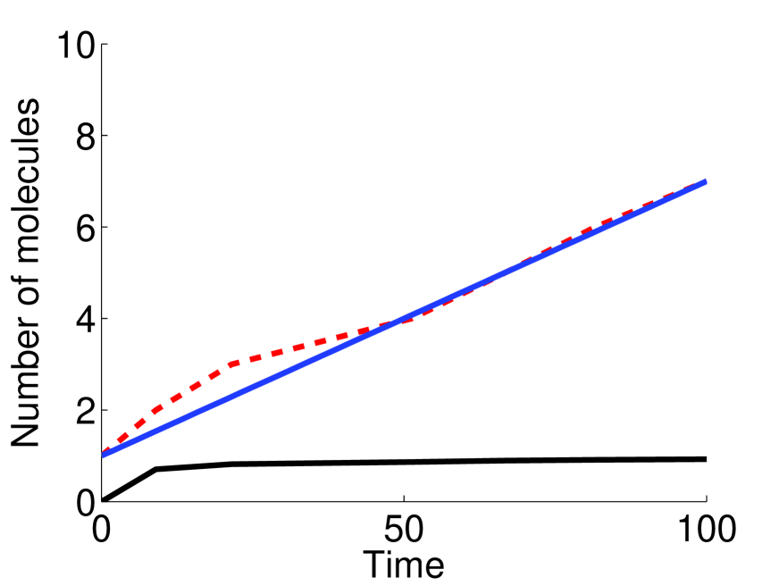
Figure 3: (Color online) Temporal evolution of the mean number of molecules $\bar{n}(t)$ (dashed (red) line) and the Fano factor (the lower solid (dark) line), and the $\alpha$-variable (the solution of Eq.(30), (the upper solid (blue) line) for the process of bacterial chemosensing with the same set of parameters as in Fig.(1).

The allosteric model describes a cluster of $N$ Tar receptor dimers with $M$ methylation sites. Addition or removal of methyl groups take place at rates $k_{r}(1-a_{n})$ or $k_{b}a_{n}$. The cluster activity depends on the ligand concentration $L$ and the methylation state as $a_{n}=\frac{1}{1+e^{f(n,L)}}$ with the free energy $f(n,L)=\gamma(n_{0}-n)+N\ln\frac{1+L/K_{off}}{1+L/K_{on}}$, where $K_{on}$ and $K_{off}$ are the dissociation constants of ligand to the active and inactive receptors respectively.

Let us now apply the Poisson representation technique. The chemical master equation (29) describes a one-step reaction process and for slowly varying $a_{n}$ (provided $\gamma\ll 1$) it is the case of monomolecular reactions (9). The equation for the Poissonian $\alpha$ variable follows as

$$\dot{\alpha}=k_{r}(1-a(\alpha))+k_{b}a(\alpha).$$ (30)

There is no noise term in this equation which means that the probability distribution function remains Poissonian

$$P(n,t)=\frac{[\alpha(t)]^{n}e^{-\alpha(t)}}{n!}$$ (31)

with $\alpha(t)$ being the solution of the Eq.(30). Figures (1) and (2) display the temporal evolution of the probability distribution function.

In order to find out how well the Poisson distribution describes this stochastic process of bacterial chemosensing we perform numerical simulations of the master equation (29) using the well-known Gillespie algorithm gillespie_alg . Figure 3 pictures temporal dynamics of the mean number of molecules $\bar{n}(t)$ and the quantity $\frac{[n(t)-\bar{n}(t)]^{2}}{\bar{n}(t)}$ (the Fano factor) which should be equal to one for the Poisson distribution. For comparison we also plot the time evolution of the solution of Eq.(30) for the $\alpha$-variable. Taking into account that the number of particles is small (which means that the fluctuations could be large) we conclude that, first, the statistics of the process rapidly approaches Poissonian and, second, the analytical solution (31) to the master equation (29) describes the process quite well.

An open question though remains how to apply an integral fluctuation relation in order to investigate responses to signals celani as well as various cases of feedback control in the case of pure Poisson stochastic process. We will leave that for further research stressing here that it was important to show that the model of bacterial chemosensing could be efficiently studied using the Poisson representation technique.

V.2 Fluctuations in molecular evolution

Let us now consider an evolution of a finite population composed of $N$ binary purine/pyrimidine sequences, of length $L$. We begin with the following master equation for the probability distribution $P({n_{\xi}},t)$ as a function of the set of occupation numbers ${n_{\xi}}$ $(0\leq\xi\leq L)$ for the finite population Crow-Kimura model deem

$$\dot{P}(\{n_{\xi}\}) = \frac{1}{N}\sum_{\xi\neq\xi^{\prime}}r(\xi)[(n_{\xi}-1)(n_{\xi^{\prime}}+1)P(n_{\xi}-1,n_{\xi^{\prime}}+1)$$ (32)

$$- n_{\xi}n_{\xi^{\prime}}P(\{n_{\xi}\})]$$

$$+ \mu\sum^{L}_{\xi=0}[(L-\xi)(n_{\xi}+1)P(n_{\xi}+1,n_{\xi+1}-1)$$

$$+ \xi(n_{\xi}+1)P(n_{\xi-1}-1,n_{\xi}+1)-Ln_{\xi}P(\{n_{\xi}\})]$$

$$+ \nu\sum^{L}_{\xi=0}[\rho_{+}(L-\xi)(n_{\xi}+1)P(n_{\xi}+1,n_{\xi+1}-1)$$

$$+ \xi\rho_{-}(n_{\xi}+1)P(n_{\xi-1}-1,n_{\xi}+1)$$

$$- n_{\xi}(\rho_{+}(L-\xi)+\rho_{-}\xi)P(\{n_{\xi}\})],$$

where $r(\xi)=Lf(\xi)$ is the replication rate, $\mu$ is the rate of point mutation, or of single base substitution, $\nu$ is the rate of horizontal gene transfer of single letters between an individual sequence and the population. $\rho_{\pm}=(1\pm u)/2$ is the probability of inserting a wild-type or nonwild-type letter by horizontal gene transfer, where $u=\frac{1}{N}\sum^{L}_{\xi=0}(2\xi/L-1)n_{\xi}$ is the ”average base composition” deem .

The master equation describes the following individual-based model of evolution which includes the following replication, point mutation, and horizontal gene transfer events $\xi+\xi^{\prime}\begin{array}[]{c}r(\xi)/N\\ \longrightarrow\\ \cdot\end{array}\xi+\xi$, $\xi\begin{array}[]{c}\mu(L-\xi)\\ \longrightarrow\\ \mu\xi\end{array}\xi\pm 1$, and $\xi\begin{array}[]{c}\nu\rho_{+}(L-\xi)\\ \longrightarrow\\ \nu\rho_{-}\xi\end{array}\xi\pm 1$, respectively.

The FPE for the quasiprobability function $f(\{\alpha_{\xi}\},t)$ that is equivalent to the master equation (32) in the Poisson representation reads as

$$\dot{f}(\{\alpha_{\xi}\},t)=-\sum_{\xi}\frac{\partial}{\partial\alpha_{\xi}}\left[A_{\xi}f(\{\alpha_{\xi}\},t)\right]$$

$$+\frac{1}{2}\sum_{\xi\xi^{\prime}}\frac{\partial^{2}}{\partial\alpha_{\xi}\partial\alpha_{\xi}^{\prime}}\left[B_{\xi\xi^{\prime}}f(\{\alpha_{\xi}\},t)\right]$$ (33)

The deterministic term of the stochastic differential equations corresponding to the above FPE leads to

$$\dot{\alpha}_{\xi}=A_{\xi}=\mu[(L-\xi+1)\alpha_{\xi-1}+(\xi+1)\alpha_{\xi+1}-L\alpha_{\xi}]$$

$$+\nu[\rho_{+}(L-\xi+1)\alpha_{\xi-1}+\rho_{-}(\xi+1)\alpha_{\xi+1}$$

$$-((L-\xi)\rho_{+}\xi\rho_{-})\alpha_{\xi}]+[r(\xi)-\sum^{L}_{\xi^{\prime}=0}r(\xi^{\prime})\alpha_{\xi^{\prime}}]\alpha_{\xi}$$

that corresponds to the population level model for infinite population quasispecies theory deem . The fluctuation diffusion matrix can be obtained from the FPE (33) without the system size expansion thus being exact for any finite $N$ (see Appendix B):

$$B=\left(\begin{array}[]{cc}\frac{2L}{N}f(\xi)\alpha_{\xi}\alpha_{\xi^{\prime}}&-\frac{L}{N}[f(\xi)+f(\xi^{\prime})]\alpha_{\xi}\alpha_{\xi^{\prime}}\\ -\frac{L}{N}[f(\xi)+f(\xi^{\prime})]\alpha_{\xi}\alpha_{\xi^{\prime}}&\frac{2L}{N}f(\xi^{\prime})\alpha_{\xi}\alpha_{\xi^{\prime}}\\ \end{array}\right)$$ (36)

In the weak noise limit the above presented framework can be applied to the molecular evolution process to obtain the probability distribution in the form of (20) having the deterministic drift and the fluctuation diffusion matrices variables substituted with species populations $n_{\xi}$. This, in turn, will allow to get the integral fluctuation relation (28) for the finite population Crow-Kimura model. An integral fluctuation theorem was already applied to evolutionary processes lassig . Our approach makes it possible to study related processes for finite populations without system size expansion and in time-varying environments or under some feedback control.

VI Conclusion

In summary, our paper contains following new results:

1. It presents a novel framework to investigate various non-equilibrium nonlinear systems with a truly wide range of applications, including (bio)chemical reactions, ecology, epidemiology, and molecular evolution. This approach allows to derive time-dependent probability distribution function for variables of finite open stochastic systems without a system-size approximation.

2. It shows that a non-equilibrium free energy and some functionals can serve as Lyapunov functions, which has an important property to de- cay to its minimal value monotonously at all times. The next challenge might be to consider the non-equilibrium Lyapunov function(s) to get some insight into various non- linear stochastic (e.g., the evolutionary) processes.

3. It contains a novel, rather generalized, integral fluctuation relation (Eq.25) for nonlinear non-equilibrium systems including those under feedback control.

   Please note that our Eq. (25) is different from the equation considered by Jarzynski jarzynski in which there is no feedback control. Our Eq. (25) is also different from the equation considered by Sagawa and Ueda sagawa , which can be applied only to equilibrium systems.

Our paper contain many new results and advance substantially the field of non-equilibrium statistical physics, especially small or finite open systems. The applications presented in the paper, the processes of bacterial chemosensing described by the Monod-Wyman- Changeux allosteric model and the Crow-Kimura model of molecular evolution, are in the focus of current research activities in leading world labs. The approach presented in the paper makes it much easier to deal with those problems.

We thank P. Grassberger for valuable discussions, G. Hu, H. Orland and T. Sagawa for reading some parts of the manuscript and useful comments, and M. Deem for useful conversations. This work was supported by the National Science Council in Taiwan under Grant Nos. NSC 100-2112-M-001-003-MY2, NSC 101-2811-M-001-104, and NCTS in Taiwan.

Appendix A Derivation of the integral fluctuation relation

Let us derive the fluctuation relation (28). We begin with

$$\left\langle e^{-\frac{1}{\epsilon}(\Delta H-\Delta F)-I}\right\rangle=\int dx_{0}dyP(x_{0})P(y|x)e^{-\frac{\Delta H-\Delta F}{\epsilon}-I}$$

where we have defined the change of the non-equilibrium free energy and of the Hamiltonian as $\Delta F=F(\lambda)-F_{0}(\lambda)$ and $\Delta H=H(x_{t},\lambda_{t})-H(x_{0},\lambda_{0})$. The mutual information is $I(x,y)=\ln\frac{P(y|x)}{P(y)}$ cover_thomas ; $P(x_{0})$ and $P(y|x)$ are the initial and conditional probability distribution functions. Then we follow the lines presented in sagawa

$$\int dx_{0}dyP(x_{0})P(y|x)e^{-\frac{1}{\epsilon}(\Delta H-\Delta F)-I}$$

$$=\int dx_{0}dyP(x_{0})P(y|x)e^{-\frac{1}{\epsilon}(H(x_{t},\lambda_{t})-H(x_{0},\lambda_{0}))}e^{\frac{1}{\epsilon}\triangle F}\frac{P(y)}{P(y|x)}$$

$$=\int dx_{0}dyP(x_{0})P(y|x)e^{-\frac{1}{\epsilon}(H(x_{t},\lambda_{t})-H(x_{0},\lambda_{0}))}\frac{Z_{0}}{Z_{t}}\frac{P(y)}{P(y|x)}$$

$$=\int dx_{0}dy\frac{e^{-\frac{1}{\epsilon}H(x_{t},\lambda_{t})}}{Z_{t}}P(y)=\int dx_{t}\frac{e^{-\frac{1}{\epsilon}H(x_{t},\lambda_{t})}}{Z_{t}}=1.$$

The last calculation step used the Liouville s theorem $dx_{0}=dx_{t}$ goldstein . Thus we obtain the integral fluctuation relation

$$\left\langle e^{-\frac{1}{\epsilon}(\Delta H-\Delta F)-I}\right\rangle=1.$$

Appendix B Fluctuation diffusion matrix for the finite population Crow-Kimura model

The FPE (33) can be derived straightforwardly using the Eq. (7) for the set of ”reactions”, just as (4), involving replication, point mutation and horizontal gene transfer processes. It is easy to see that only the replication events $\xi+\xi^{\prime}\begin{array}[]{c}r(\xi)/N\\ \longrightarrow\\ \cdot\end{array}\xi+\xi$ and $\xi+\xi^{\prime}\begin{array}[]{c}r(\xi^{\prime})/N\\ \longrightarrow\\ \cdot\end{array}\xi^{\prime}+\xi^{\prime}$, where $r(\xi)=Lf(\xi)$, contribute to the noise diffusion matrix elements $B_{\xi\xi^{\prime}}$ as they involve bi-reagent interactions. After some simple algebra without any approximation the $B$ matrix takes the following exact form

$$B=\left(\begin{array}[]{cc}\frac{2L}{N}f(\xi)\alpha_{\xi}\alpha_{\xi^{\prime}}&-\frac{L}{N}[f(\xi)+f(\xi^{\prime})]\alpha_{\xi}\alpha_{\xi^{\prime}}\\ -\frac{L}{N}[f(\xi)+f(\xi^{\prime})]\alpha_{\xi}\alpha_{\xi^{\prime}}&\frac{2L}{N}f(\xi^{\prime})\alpha_{\xi}\alpha_{\xi^{\prime}}\\ \end{array}\right)$$ (39)

References

• (1) I. Prigogine and G. Nicolis, Self-Organization in Non-Equilibrium Systems (Wiley, 1977).
• (2) H. Haken, Synergetics: Introduction and Advanced Topics (Springer, 2012).
• (3) R.L. Stratonovich, Nonlinear Nonequilibrium Thermodynamics (Springer, 1992).
• (4) J. Keizer, Statistical Thermodynamics of Nonequilibrium Processes (Springer, 1987).
• (5) W.-J. Ma and C.-K. Hu, J. Phys. Soc. Jpn. 79, 024005, 024006, 054001, and 104002 (2010).
• (6) M.-C. Huang, J.-W. Wu, Y.-P. Luo, and K.G. Petrosyan, J. Chem. Phys. 132, 155101 (2010).
• (7) Y.-C. Hung and C.-K. Hu, Comput. Phys. Commun. 182, 249 (2011).
• (8) G. Hu, Physica A 132, 586 (1985); G. Hu, Phys. Lett. A 110, 253 (1985); G. Hu, Phys. Rev. A 36, 5782 (1987).
• (9) H. Qian and M. Qian, Phys. Rev. Lett. 84, 2271 (2000).
• (10) H. Qian, J. Phys. Chem. B 106 2065 (2002).
• (11) H. Qian, J. Phys. Chem. B 110, 15063 (2006).
• (12) N.G. van Kampen, Stochastic Processes in Physics and Chemistry, 3rd ed. (Elsevier, Amsterdam, 2007).
• (13) D.T. Gillespie, Ann. Rev. Phys. Chem. 58, 35 (2007).
• (14) C.W. Gardiner and S. Chaturvedi, J. Stat. Phys. 17, 429 (1977); S. Chaturvedi and C.W. Gardiner, J. Stat. Phys. 18, 501 (1978).
• (15) C.W. Gardiner, Handbook of Stochastic Methods, 3rd ed. (Springer, 2004).
• (16) C.W. Gardiner and P. Zoller, Quantum Noise, 3rd ed. (Springer, 2004).
• (17) E. Smith, Rep. Prog. Phys. 74, 046601 (2011).
• (18) K. Friston, Nat. Rev. Neurosci. 11, 127 (2010); Entropy 14, 2100 (2012).
• (19) B. Gaveau and L.S. Schulman, Phys. Lett. A 229, 347 (1997).
• (20) Yu.L. Klimontovich, Physics-Uspekhi 42, 375 (1999) and references therein.
• (21) M. Esposito and C. Van den Broeck, Europhys. Lett. 95, 40004 (2011).
• (22) S. Deffner and E. Lutz, arXiv:1201.3888 [cond-mat.stat-mech] (2012).
• (23) J. Monod, J. Wyman, and J.-P. Changeux, J. Mol. Biol. 12, 88 (1965); J.-P. Changeux and S.J. Edelstein, Science 308, 1424 (2005).
• (24) A. Celani and M. Vergassola, Phys. Rev. Lett. 108, 258102 (2012).
• (25) M. Flores, T.S. Shimizu, P.R. ten Wolde, and F. Tostevin, Phys. Rev. Lett. 109, 148101 (2012).
• (26) J. F. Crow and M. Kimura, An Introduction to Population Genetics Theory (Harper and Row, New York, 1970); D. B. Saakian and C.-K. Hu, Phys. Rev. E 69, 046121 (2004).
• (27) J.-M. Park and M.W. Deem, Phys. Rev. Lett. 98, 058101 (2007); J.-M. Park, E. Munoz, and M.W. Deem, Phys. Rev. E 81, 011902 (2010); M.W. Deem, Annu. Rev. Condens. Matter Phys. 4, 287 (2013).
• (28) See also P.D. Drummond, T.G. Vaughan, and A.J. Drummond, J. Phys. Chem. A 114, 10481 (2010) for recent application of the technique to autocatalytic systems.
• (29) R. Graham and T. Tel, Phys. Rev. A 31, 1109 (1985); J. Stat. Phys. 35, 729 (1984).
• (30) H. Touchette, Physics Reports 478, 1 (2009).
• (31) L.J. Curtis, Am. J. Phys. 43, 1101 (1975).
• (32) H. Goldstein, Classical Mechanics, 2nd ed. (Addison Wesley, 1980).
• (33) S. Kullback, Information Theory and Statistics (Peter Smith, Gloucester, 1978).
• (34) A.M. Yaglom, Mat. Sb. 24, 457 (1949).
• (35) T.M. Cover and J.A. Thomas, Elements of information theory (Wiley, 1991).
• (36) T. Sagawa, Journal of Physics: Conference Series 297, 012015 (2011).
• (37) C. Jarzynski, Phys. Rev. Lett. 78, 2690 (1997).
• (38) T. Sagawa and M. Ueda, Phys. Rev. Lett. 104, 090602 (2010).
• (39) D.T. Gillespie, J. Comput. Phys. 22, 403 (1976); J. Phys. Chem. 81, 2340 (1977).
• (40) V. Mustonen and M. Lassig, PNAS 107, 4248 (2010).