The resonant dynamics of arbitrarily-shaped meta-atoms

Abstract

Meta-atoms, nano-antennas, plasmonic particles and other small scatterers are commonly modeled in terms of their modes. However these modal solutions are seldom determined explicitly, due to the conceptual and numerical difficulties in solving eigenvalue problems for open systems with strong radiative losses. Here these modes are directly calculated from Maxwell’s equations expressed in integral operator form, by finding the complex frequencies which yield a homogenous solution. This gives a clear physical interpretation of the modes, and enables their conduction or polarization current distribution to be calculated numerically for particles of arbitrary shape. By combining the modal current distribution with a scalar impedance function, simple yet accurate models of scatterers are constructed which describe their response to an arbitrary incident field over a broad bandwidth. These models generalize both equivalent-dipole and and equivalent-circuit models to finite sized structures with multiple modes. They are applied here to explain the frequency-splitting for a pair of coupled split rings, and the accompanying change in radiative losses. The approach presented in this paper is made available in an open-source code.

I Introduction

Resonances are fundamental to many modern photonic and electromagnetic systems, including metamaterials, nano-antennas, and plasmonic and dielectric oligomers, all of which seek to strongly manipulate scattering using small elements. For example, the negative index of a metamaterial is usually associated with a resonance in the magnetic polarizability of the constituent meta-atoms. Typical nano-antenna designs consist of coupled metallic rods operating near their resonance. Fano resonances arise in plasmonic oligomers due to interference between the modes of the coupled system. The resonant nature of these systems makes it highly desirable to create simple oscillator models to describe their dynamics. Although not necessarily having dimensions much smaller than the wavelength, the building blocks of these systems are typically not large compared to the wavelength, thus they can be adequately described by a small number of modes.

For metamaterials consisting of a large, three-dimensional array, much effort has been dedicated to homogenization approaches, whereby the metamaterial is approximated by a continuous medium, and the system is described in terms of average fields Simovski (2011). However, in many systems of interest, the required criteria for homogenizability are not satisfied, either because the meta-atoms are not sufficiently sub-wavelength, the arrays are so small that boundary effects and radiation losses are very strong, or the arrangement is not periodic. As an alternative to homogenization, it is possible to consider the fields of a metamaterial’s Bloch modes as the fundamental degrees of freedom Zeng et al. (2012), however this suffers from many of the same limitations. In many cases the modes of individual resonators form a much more convenient basis to study the behavior of meta-atoms and resonant scatterers, since the number of excited modes is typically small. For many experimental configurations reported in the literature, the number of scatterers in the system is small enough that it is feasible to explicitly describe the modal excitation of each of them.

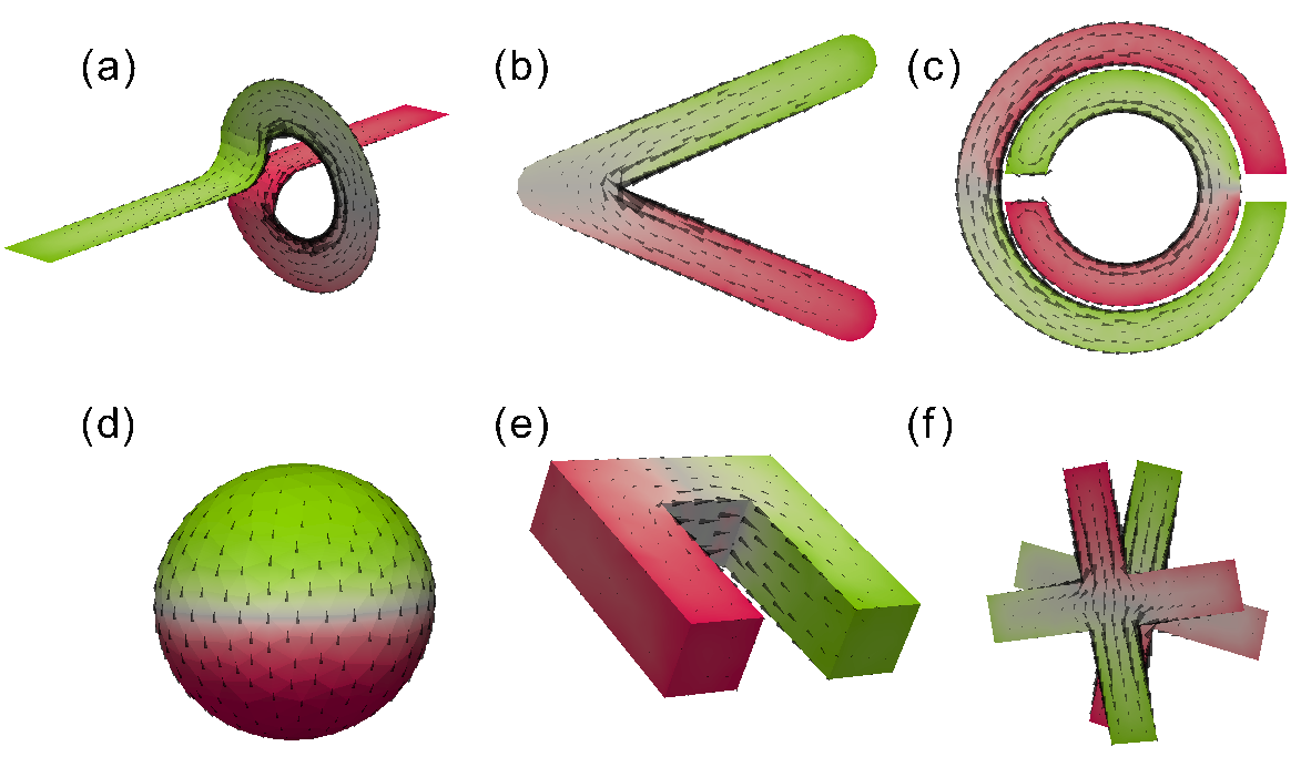
Figure 1: (Color online) Meta-atoms each showing charge (colors) and current (arrows) distributions for one of their modes. (a) Canonical spiral, (b) V-antenna, (c) split-ring resonator, (d) sphere, (e) horseshoe and (f) twisted crosses.

In this article, the modes of arbitrarily-shaped resonant particles are found and are used to construct simple oscillator models. These models give a highly accurate description of the particles over a very broad bandwidth and directly include radiative effects. They satisfy causality, and can account for the coupling between particles, which gives rise to hybridized modes. Examples of applicable structures and their modes are shown in Fig. 1. For all of these structures the fundamental modes are plotted, except in Fig. 1(f), where a second-order mode is shown. Routines to calculate the coefficients of the oscillator model from the scatterer geometry are implemented in an open-source software package OpenModes ope .

This paper is organized as follows. In Section II, existing approaches to find the modes of open resonators are discussed, leading to the proposed approach which is presented in Section III. In Section IV, this model is used to solve the problem of coupled resonators, showing how the influence of multiple modes of each uncoupled resonator can easily be taken into account in the hybridization process. Appendix A gives details of the EFIE operator used, Appendix B gives general details of the numerical implementation, and Appendix C outlines the procedure to find the singularities.

II The physics of open resonators and their modes

The simplest approach to finding the modes of resonant particles is to illuminate the structure at a frequency corresponding to a resonance, and observe the fields either through numerical simulation, or with experimental techniques such as near-field scanning microscopy Alonso-Gonzalez et al. (2011). These approaches work well if the modes are greatly separated in frequency, however many systems operate in a regime of overlap or interference between different modes Miroshnichenko et al. (2010), and it is difficult to distinguish the contribution of each mode to the total response. To develop a model for the resonances in meta-atoms or plasmonic structures, a simple and appealing approach is to develop equivalent circuit models Bilotti et al. (2007); Ikonen and Tretyakov (2007); Karyamapudi (2005); Staffaroni et al. (2012). This has the advantage of providing insight and computational simplicity, and builds on well established results in antenna and microwave theory. However, such a circuit model must be developed manually for each different meta-atom type, and important physical phenomena such as coupling to radiated fields are not adequately described by lumped circuit elements.

Models which represent the particles by their dipole moments have been constructed for meta-atoms, and these can gives a reasonable description of the far-field coupling of the fundamental modes, including radiation effects Sersic et al. (2011). The most well-studied case using dipole or multipole methods is that of a sphere embedded in a uniform background, since it has a multipole solution which describes the polarization of each mode in closed form Bohren and Huffman (1983a). However, many practical systems have resonators which are of much lower symmetry, either through deliberate design or the presence of a perturbing substrate, and the modes of complex-shaped resonators can have significant contributions from many multipole terms Krasnok et al. (2014). Particularly for near-field interaction effects, all of these higher-order terms must be included in calculations, thus the multipole approach loses its simplicity. To model such systems effectively, analytical methods cannot be used to find the eigenmodes, and some other solution must be found. For plasmonic particles, it is possible to find the modes numerically under the quasi-static approximation Mayergoyz et al. (2005). This approach makes very strong assumptions about the sub-wavelength nature of the particle, and radiation effects are neglected, although they may be added back to the model as a perturbation Davis et al. (2009).

In closed cavities, modes can be found by expressing Maxwell’s equations in eigenvalue form, with the eigenvalues corresponding to the resonant frequencies. However, meta-atoms and nano-antennas are intrinsically open systems, which radiate into the surrounding environment. Their modal near fields are not strictly confined to any well-defined region of space, and must somehow be disentangled from the radiating fields. Particularly for plasmonic particles, their may also be strong dissipative losses. Thus it is not appropriate to solve the lossless problem and to treat radiative and dissipative losses as a perturbation, since they can induce strong qualitative changes in the response of a system Yakovlev and Hanson (2000); Davoyan et al. (2010).

In the language of Hamiltonian mechanics, these significant losses mean that the system must be described by a non-Hermitian operator. In fields such as quantum optics, open systems have been studied using the “system and bath” approach Viviescas and Hackenbroich (2003). In this model, the system is partitioned into a resonant system and a continuum of modes, and coupling terms between the two are introduced. Although this description is complete, one drawback is that the partitioning of the system is not unique, thus the modes are not uniquely defined. Additionally, it is necessary to include an infinite continuum of plane waves into the calculations, which is somewhat cumbersome, and cannot be considered as a simple oscillator model. Similar models incorporating the complete spectrum of plane waves have been utilized for metamaterials Jenkins and Ruostekoski (2012), under the assumption that each meta-atom is described by a single electric and magnetic dipole moment.

An alternative approach is to study the quasi-normal modes, which are self-consistent undriven solutions occurring at complex values of frequency. They extend the familiar concept of resonant modes to dissipative systems, and although such modes are not orthogonal in the usual sense, in certain cases they do satisfy orthogonality over an unconjugated inner product Leung et al. (1994). Such modes seem to offer an intuitive description for resonant systems, however, not only are they not-well confined, their fields actually diverge with increasing distance from the resonator. This corresponds to temporal solutions as $t\rightarrow\infty$, where almost all energy has escaped from the cavity into radiated fields Kristensen et al. (2012). By utilizing appropriate absorbing boundary conditions this divergence can be handled Sauvan et al. (2013); Bai et al. (2013), however this spatially divergent field is an inconvenient representation of a compact object. In Ref. Bai et al., 2013 it was shown that absorption, scattering and emission effects can be calculated from quasi-normal modes, and it is noteworthy that the all the relevant formulas effectively integrate the polarization current over the volume of the scatterer.

Integral equation approaches which solve for currents are routinely used in scattering theory, and the singularities of the scattering operator can also yield solutionsHanson and Yakovlev (2002), which are essentially the same as quasi-normal modes. In Ref. Kovalyov and Ponomarev, 2011 these were calculated based on a spherical harmonic decomposition. This approach is well suited to modeling antennas or scatterers separated by relatively large distances, and all far-field radiation channels are explicitly incorporated. However, spherical harmonics are is not suitable for modeling the strongly varying near-fields which couple meta-atoms together, nor the influence of an inhomogeneous background, and this also involves an arbitrary and non-physical partitioning of space into internal and external parts. For open resonators which are uniform along one direction, a comprehensive theory was presented in Ref. Shestopalov and Shestopalov, 1996, however this restriction excludes many structures of practical interest.

The advantage of the scattering approach is that the solution is given in terms of the conduction or polarization current only within the resonant structure. This gives a more useful description of the mode, since currents remains finite at complex frequencies, in contrast to the corresponding fields which diverge. The natural approach to solving for the current on the resonator directly is to use integral equation approaches, known variously in the literature as the method of moments Harrington (1968); Gibson (2008), boundary element method or integral equation method. In these approaches, the current is expanded into a finite number of basis functions, and a Green’s function is used to calculate the interaction between all the current elements. By solving the resulting impedance matrix, the solution can be found for any external exciting field, and the radiation boundary conditions are automatically taken into account. Such approaches are well-established for solving microwave scattering problems, and more recently they have been applied successfully to dielectric and plasmonic nano-structures Kern and Martin (2009); Ergül (2012); Zheng et al. (2013a). It is important to emphasize that while these approaches use the terminology of impedance taken from circuit theory, it was shown in Ref. Greffet et al., 2010 that it has an alternative interpretation related to the local density of states.

Modes of the structure correspond to the singularities of the impedance matrix in the complex plane, and these have been found for dielectric resonators Glisson et al. (1983), and have been used to describe the transient scattering of a radar pulse from a target Baum (1976, 1978). This approach can be understood as applying analytical continuation to the eigenvalue expansion, which provides a scalar description of the structure, but which must be recalculated at each frequency of interest. In Ref. Zheng et al., 2013a such an eigenvalue expansion was applied the impedance matrix in order to calculate the excitation and coupling of plasmonic dolmen structures. In Ref. Mäkitalo et al., 2014 the properties of the Müller formulation of the surface integral problem were studied in detail, and it was shown that the singularities of the integral operator can yield the resonances of plasmonic structures in both full-wave and quasi-static regimes. In Ref. Zheng et al., 2013b the location of the singularities of plasmonic structures in the complex frequency was related to the quality factor and the stored energy in the near-fields of the structure. In the next section a procedure for finding these singularities will be presented, and they will be used to develop a simple oscillator model accounting for all excitation, coupling, radiation and interference effects.

III Modeling a single element

In this section a numerical model is constructed for an individual resonant element. It is then shown how analyzing the frequencies where the impedance matrix is singular yields a compact model which is accurate over a broad bandwidth, and describes each mode with quite simple dynamics.

III.1 The electric field integral equation

All dynamic quantities have implicit time dependence of $\exp(st)$ with $s=\Omega+j\omega$, and are related to time domain quantities via a two-sided Laplace transform pair Baum (1978). The electric field $\mathbf{E}_{s}$ scattered by an object is related to its induced currents $\mathbf{j}$ via the electric field integral equation (EFIE):

$$\mathbf{E}_{s}\left(\mathbf{r},s\right)=\iiint_{\Gamma}\overline{\overline{G}}_{0}(\mathbf{r}-\mathbf{r}^{\prime},s)\cdot\mathbf{j}(\mathbf{r}^{\prime},s)\mathrm{d^{3}\mathbf{r}}$$ (1)

where the free space dyadic Green’s function $\overline{\overline{G}}_{0}$ is given by Eq. (12), and $\Gamma$ is the volume of the object. For perfectly conducting metals considered here, the the tangential components of the scattered field and incident field $\mathbf{E}_{i}$ cancel on the surface $\hat{\mathbf{n}}\times\mathbf{E}_{i}=-\hat{\mathbf{n}}\times\mathbf{E}_{s}$, the integration is over the object surface $\partial\Gamma$ and the resulting operator equation is denoted $\mathbf{E}_{i}=\mathcal{Z}\left(\mathbf{j}\right)$. More general formulations can include polarization within dielectrics or imperfect metals, through a volume Zheng et al. (2013a) or surface equivalent problem Ylä-Oijala et al. (2005). Furthermore, if a different Green’s function is used in Eq. (1), background media can be incorporated while still only solving for currents on the scatterer, with layered media Michalski and Mosig (1997) being of particular interest. Note that artificial magnetism due to circulating currents is accounted for in Eq. (1) by the gradient of the electric field Simovski and Tretyakov (2010), without requiring the additional terms used in some models Jenkins and Ruostekoski (2012); Sersic et al. (2011).

In Ref. Hanson and Yakovlev, 2002 the properties of such integral operators are discussed in detail, using the tools of functional analysis. In particular the spectral properties of such operators are discussed, which are relevant to the techniques used in this section. Although many of the relevant proofs are not directly applicable to Eq. (1), the uniqueness theorem means that the solutions found are genuine physical properties which are independent of the particular formulation of Maxwell’s equations which is used. To solve the operator equation numerically, the geometry is represented by a triangular surface mesh and the current is expanded into basis functions $\mathbf{f}_{n}$, each defined over an area $T_{n}$

$$\mathrm{\mathbf{j}}\left(\mathbf{r}\right)=\sum_{n=1}^{N}I_{n}\mathbf{f}_{n}\left(\mathbf{r}\right).$$ (2)

To obtain a finite number of equations, the incident field is weighted by the same set of basis functions

$$V_{n}=\iint_{T_{n}}\mathbf{f}_{n}\left(\mathbf{r}\right)\cdot\mathbf{E}_{i}\left(\mathbf{r}\right)\mathrm{d^{2}}\mathbf{r}.$$

Applying the same procedures to Eq. (1) results in a matrix equation which describes the full dynamics

$$\mathrm{V}(s)=\mathrm{Z}(s)\cdot\mathrm{I}(s),$$ (3)

where $\mathrm{V}$ and $\mathrm{I}$ are vectors of length $N$, whilst $\mathrm{Z}$ is the $N\times N$ impedance matrix which approximates the operator $\mathcal{Z}$, and is defined in Eq. (13).

The impedance matrix is closely related to the interaction matrix in coupled-dipole models Sersic et al. (2011), but it has the advantage of directly including both mutual and self-interaction effects. It is sometimes useful to separate it into two parts according to the dominant frequency dependence, which is equivalent to separating the contributions of the scalar and vector potentials in the Lorenz gauge

$$\mathrm{Z}\left(s\right)=s\mathrm{L}\left(s\right)+\frac{1}{s}\mathrm{S}\left(s\right).$$ (4)

In the limit $\gamma|\mathbf{r}|\rightarrow 0$ (where $\gamma=s\sqrt{\varepsilon\mu}$ is the complex propagation factor), these matrices correspond to the inductance and elastance (the inverse of capacitance) respectively, hence the symbols for the corresponding scalar quantities are used Kennelly (1936). Due to Lorentz reciprocity and the use of identical basis and weighting functions, $\mathrm{Z}$ is a complex-symmetric matrix, in the sense $Z_{mn}=Z_{nm}$, but in general $Z_{mn}\neq\overline{Z}_{nm}$ (the bar denotes complex conjugation).

III.2 Modes as frequency-dependent eigenvectors

From the impedance matrix $\mathrm{Z}(s)$, a simple model can be extracted at each frequency, by solving the eigenvalue problem

$$\mathrm{Z}(s)\cdot\mathrm{I}^{(\alpha)}\left(s\right)=z^{(\alpha)}\left(s\right)\mathrm{G}\cdot\mathrm{I}^{(\alpha)}\left(s\right),$$ (5)

where the eigenvalue $z^{(\alpha)}(s)$ is a scalar impedance, and the eigenvector $\mathrm{I}^{(\alpha)}\left(s\right)$ gives the corresponding current distribution. The matrix equation (5) is a numerical approximation of the operator eigenvalue equation $\mathcal{Z}\left(\mathbf{j}^{\left(\alpha\right)}\right)=z^{(\alpha)}\mathcal{I}\left(\mathbf{j}^{\left(\alpha\right)}\right)$, where $\mathcal{I}$ is the identity operator. Since the basis and testing functions are not orthonormal, the matrix form of the identity operator is the Gram matrixHarrington (1968); Bekers et al. (2009) $\mathrm{G}$, where $G_{mn}=\int_{T_{m}}\int_{T_{n}}\mathbf{f}_{m}\left(\mathbf{r}\right)\cdot\mathbf{f}_{n}\left(\mathbf{r}\right)\mathrm{d^{2}}\mathbf{r}$. Some works Zheng et al. (2013a); Baum (1978) use the identity matrix for this term, thus the eigenvalues may have have contributions related to the mesh density, in addition to the those from the dynamics of the physical system.

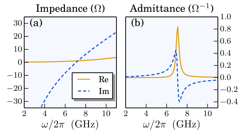
Figure 2: (Color online) (a) Eigenvalue for the first mode of an SRR, having dimensions of impedance, and (b) its inverse which has dimensions of admittance, with a Lorentzian-like shape.

Once the eigenvectors are scaled such that they satisfy the orthonormality relationship

$$\iint\limits_{\partial\Gamma}\mathbf{j}^{(\alpha)}\left(\mathbf{r}\right)\cdot\mathbf{j}^{(\beta)}\left(\mathbf{r}\right)\mathrm{d^{2}}\mathbf{r}=\mathrm{I^{(\alpha)}}^{\mathrm{T}}\left(s\right)\cdot\mathrm{G}\cdot\mathrm{I}^{(\beta)}\left(s\right)=\delta_{\alpha\beta},$$ (6)

the impedance matrix has the decomposition Hanson and Yakovlev (2002)

$$\mathrm{Z}(s)=\sum_{\alpha=1}^{N}z^{(\alpha)}\left(s\right)\mathrm{I^{(\alpha)}}\left(s\right)\otimes\mathrm{I}^{(\alpha)}\left(s\right),$$ (7)

where in practice only $\tilde{N}$ modes ($1\leq\tilde{N}\ll N$), contribute significantly to the response, and in many cases $\tilde{N}=1$ is sufficient. An arbitrary current is decomposed into a series of modes by the projection dyad $\mathrm{I^{(\alpha)}}(s)\otimes\mathrm{I}^{(\alpha)}(s)$ (without complex conjugation), and the mode dynamics are given by the impedance $z^{(\alpha)}(s)$. This could be understood as the sum of equivalent circuit responses, however it is important to emphasize the role of the projection dyad, which has no equivalent circuit counterpart. Due to the non-Hermitian nature of the system, the projection of the incident field onto this dyad can also contribute phase terms. Although counter-intuitive, this effect is completely physical and accounts for interference between modesHopkins et al. (2013).

To give a detailed example of this model, a single ring split-ring resonator (SRR) is considered, with inner radius 2.5 mm, outer radius 4 mm, gap width 1 mm, modeled as a thin PEC layer divided into 852 triangles. The dynamics of its first mode are governed by the eigenvalue $z^{(1)}(s)$ plotted in Fig. 2(a). It can be seen that the imaginary part of the impedance dominates, corresponding to the reactive stored energy, while the real part is much smaller, indicating that the radiation losses for this mode are relatively low. This is confirmed by Fig. 2(b), which shows the corresponding admittance $1/z^{(1)}(s)$, more clearly indicating the resonant nature of the mode and its relatively high quality factor.

The main drawback of this eigenvalue expansion is that it requires the full impedance matrix to be calculated and an eigenvalue decomposition to be performed at every frequency, thus it has the same computational requirements as a fully numerical model.

III.3 Modes as singularities of the operator equation

To develop a single model for a finite scatterer which is accurate over a wide frequency range, $z^{(\alpha)}(s)$ is extended analytically into the complex $s$ plane. Fig. 3 extends the eigenvalue in Fig. 2(a) in this manner. Its real and imaginary parts are given by the heights of the surfaces, with the black line indicating where they pass through zero. Clearly the eigenvalue goes to zero at the intersection of these two curves. At such frequencies, the impedance matrix $\mathrm{Z}$ is singular Baum (1978), corresponding to a current solution which can be sustained without any driving field [i.e. $\mathrm{V}=0$ in Eq. (3)]. In Ref. Marin, 1973 it was proven that for sufficiently smooth objects all such singularities are poles, and it was observed that in practice they are of first order, and no other terms are required to describe the dynamics.

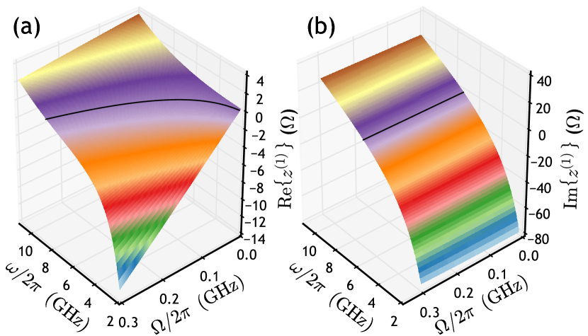
Figure 3: (Color online) (a) Real and (b) imaginary parts of the first eigenvalue of an SRR, plotted as a function of complex frequency. The solid lines show where each part is zero. Their intersection gives the complex eigenfrequency.

Since the impedance matrix $\mathrm{Z}$ has explicit dependence on $s$, the root-finding problem is nonlinear in $s$ and must be solved using iterative methods. A procedure was developed based on robust starting estimates, as detailed in Appendix C. For the example presented here, the solution converged to a relative accuracy of $10^{-8}$ within 10 iterations, making the process quite efficient. The solution of this nonlinear problem was empirically found to be more reliable than the solving frequency-dependent linear eigenvalue problem in Eq. (5), in the sense that it is much less prone to converge on a spurious non-physical eigenvalue. In Fig. 4(a) the singular points are shown for the first four modes of a split ring resonator. It can be seen that the higher order modes have have larger real parts of $s^{\left(\alpha\right)}$, indicating that they have stronger radiative losses. These singularities occur in complex-conjugate pairs, as the system response is real in the time domain.

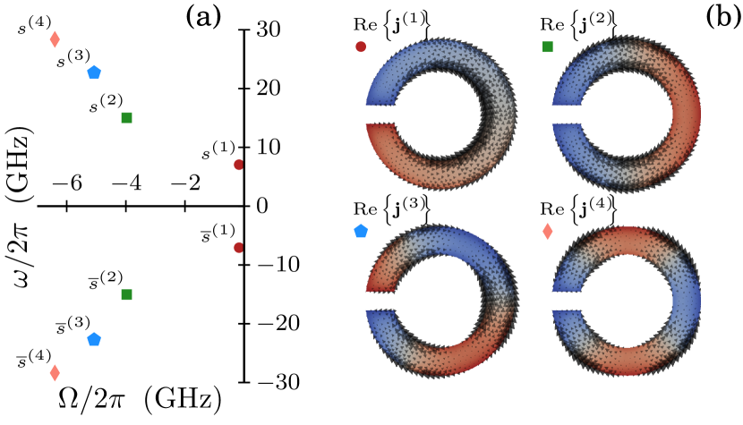
Figure 4: (Color online) (a) The complex singularities of a single split-ring resonator which give the resonant frequencies, and (b) the corresponding charge and current distributions.

For each frequency $s^{(\alpha)}$ corresponding to the resonance of a mode, there is a vector $\mathrm{I^{(\alpha)}\left(s^{(\alpha)}\right)}$ which satisfies the homogeneous equation. From this vector, the mode’s current distribution $\mathbf{j}^{(\alpha)}\left(s^{(\alpha)},\mathbf{r}\right)$ is calculated using Eq. (2), and the charge distribution is given by $q^{(\alpha)}\left(s^{(\alpha)},\mathbf{r}\right)=-\frac{1}{s^{(\alpha)}}\nabla\cdot\mathbf{j}^{(\alpha)}\left(s^{(\alpha)},\mathbf{r}\right)$. The real parts of these surface charges (colors) and currents (arrows) are shown in Fig. 1 for several different structures. Despite the strong differences in geometry, it is clear that the lowest-order modes of canonical spiral, V-antenna, sphere and horseshoe all exhibit electric dipole-like charge distributions. In Fig. 4(b) the first four modes of the single split ring resonator shown, corresponding to the singularities shown in Fig. 4(a). It can be seen that higher order modes exhibit increasing degree of spatial oscillation with increasing order, similar to the case for simple closed cavities.

These current distributions are closely linked to the frequency-dependent eigenvectors discussed in Section III.2, which can be regarded as their analytical continuation away from the singular points in the $s$ plane. In Ref. Andrew et al., 1993 it was shown that careful normalization of the eigenvectors is required for them to be analytic, and the normalization given in Eq. (6) satisfies this requirement. For the well-studied case of a sphere, the eigenvectors are frequency independent Baum (1976), although this is not true in the general case

III.4 The broadband model

The value in finding singularities in the complex $s$ plane is that they form a useful basis for modeling the dynamics of the structures. By numerically evaluating $\mathrm{d}z^{(\alpha)}/\mathrm{d}s$ at $s=s^{(\alpha)}$, and enforcing the impedance to be open-circuit at $s=0$, a fourth order model is fitted to each scalar impedance $z^{(\alpha)}$

$$z^{(\alpha)}\left(s\right)=\frac{z_{-1}^{(\alpha)}}{s}+z_{0}^{(\alpha)}+z_{1}^{(\alpha)}s+z_{2}^{(\alpha)}s^{2}.$$ (8)

These terms are all real and can be interpreted as elastance (inverse capacitance), ohmic dissipation, inductance and radiative losses respectively, and correspond directly to the form of the inverse polarizability used in dipole models Sersic et al. (2011). The advantage of this form is that the correct signs of all terms can be enforced to guarantee a passive, causal response. Many existing formulations express the admittance in terms of residues of the polesBaum (1976); Zheng et al. (2013b); Sauvan et al. (2013) of $\mathrm{Z}^{-1}$. Such models can be used instead of Eq. (8), but will be physically correct only if the residue of the conjugate pole at $s=\bar{s}^{(\alpha)}$ and the zero at the origin are correctly accounted for.

In Fig. 5 the scalar admittances $1/z^{(\alpha)}(s)$ are plotted corresponding to the modes in Fig. 4. The resonant behavior is clearly observable, and is similar to a series resonant circuit, with the real part reaching the maximum and the imaginary part crossing through zero at resonance. It can be seen that the widths of the resonant peaks increase for the higher order modes, consistent with the increased values of $\Omega$ at the singularities shown in Fig. 4(a). It is also clear that the line-shapes can be highly asymmetric, confirming that the expression in Eq. (8) is more appropriate than simpler RLC circuit or Lorentzian models.

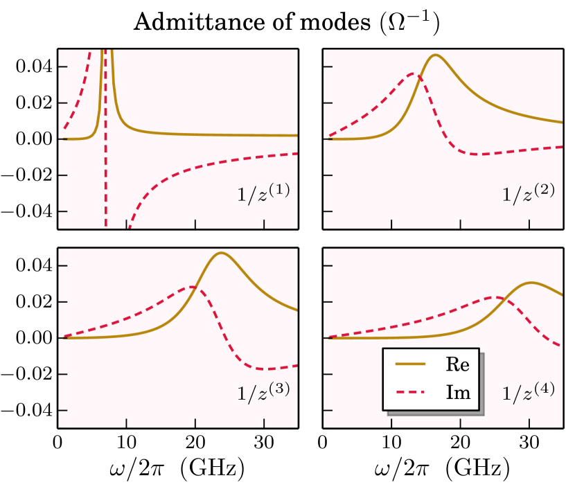
Figure 5: (Color online) Scalar admittance functions which describe the dynamics of the first four modes of a split ring resonator.

While the frequency-dependence of the eigenimpedances $z^{(\alpha)}$ is well characterized by Eq. 8, the analytic continuation of the vectors $\mathrm{I^{(\alpha)}}\left(s^{\left(\alpha\right)}\right)$ is more subtle. Each $\mathrm{I^{(\alpha)}}(s)$ is an analytic function of $s$, such that the same eigenvector can be tracked as the frequency is varied. Since they represent the Laplace transform of a real function, the currents must obey the the conjugate symmetry relationship $\mathrm{I^{(\alpha)}}(\bar{s})=\mathrm{\overline{I}^{(\alpha)}}(s)$ Baum (1975). The normalization introduced in Eq. (6) eliminates the arbitrary complex scaling factor on the eigenvectors, making it meaningful to distinguish between their real and imaginary parts. The conjugate symmetry of the eigenvectors requires that the mode currents are real on the real $s$ axis, including at zero frequency. Therefore, the presence of a non-zero imaginary part of $\mathrm{I^{(\alpha)}}$ implies that the modal current distributions cannot be frequency independent. However, from a practical point of view, all the current distributions shown in Figs. 1 and 4(a) have imaginary components (not shown) which are much smaller than the real parts, allowing their frequency variation to be neglected with little loss of accuracy.

Utilizing the vector $\mathrm{I^{(\alpha)}}\left(s^{\left(\alpha\right)}\right)$ and corresponding impedance function $z^{(\alpha)}\left(s\right)$, the response of the particle to an excitation field vector $\mathrm{V}(s)$ is well approximated by:

$$\mathrm{I}(s) = \mathrm{Z}^{-1}(s)\cdot\mathrm{V}(s)$$ (9)

$$= \sum_{\alpha=1}^{\tilde{N}}\frac{1}{z^{(\alpha)}\left(s\right)}\mathrm{I^{(\alpha)}}\left(s^{\left(\alpha\right)}\right)\left[\mathrm{I^{(\alpha)}}\left(s^{\left(\alpha\right)}\right)\cdot\mathrm{V}(s)\right],$$

III.5 Verification

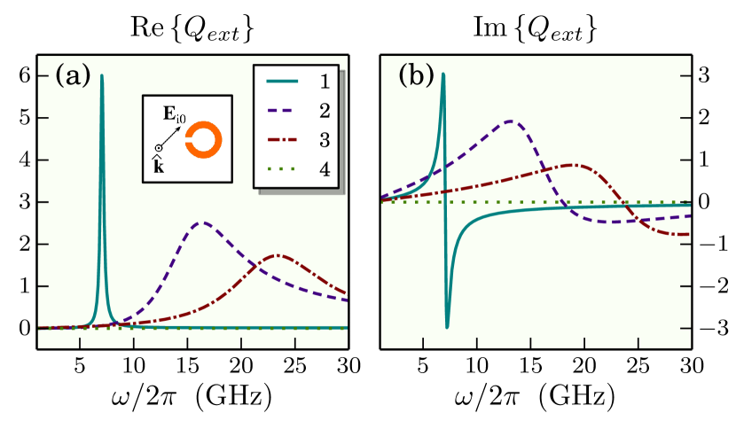
Figure 6: (Color online) The contribution of each mode to the (a) real and (b) imaginary parts of the complex extinction efficiency. The inset gives the polarization of the incident wave.

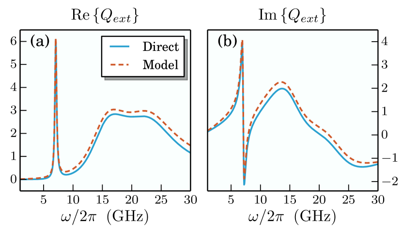
Figure 7: (Color online) Total extinction efficiency calculated from the model and compared with the direct calculation, showing the (a) real and (b) imaginary parts.

To verify the accuracy of the model, the solution obtained from Eq. (9) is compared with the exact solution of Eq. (3). The simplest quantity which characterizes the response is the extinction efficiency, which shows the energy extracted from the incident field by the scatterer. It is calculated as

$$Q_{ext} = \frac{\eta\iint_{\partial\Gamma}\mathbf{\overline{E}}_{i}\left(\mathbf{r}\right)\cdot\mathbf{j}\left(\mathbf{r}\right)\mathrm{d^{2}}\mathbf{r}}{\pi r_{o}^{2}\iint_{\partial\Gamma}\mathbf{\overline{E}}_{i}\left(\mathbf{r}\right)\cdot\mathbf{E}_{i}\left(\mathbf{r}\right)\mathrm{d^{2}}\mathbf{r}}$$ (10)

$$= \frac{\eta\overline{\mathrm{V}}\left(s\right)\cdot\mathrm{I}\left(s\right)}{\pi r_{o}^{2}\overline{\mathrm{V}}\left(s\right)\cdot\mathrm{V}\left(s\right)},$$

where $\eta=\sqrt{\frac{\mu}{\epsilon}}$ is the intrinsic impedance of the background medium, and $r_{o}$ is the radius of the smallest sphere enclosing the object . The incident field is a plane-wave described by $\mathbf{E}_{i}\left(\mathbf{r}\right)=\mathbf{E}_{i0}\exp\left(-\gamma\hat{\mathbf{k}}\cdot\mathbf{r}\right)$, where $\hat{\mathbf{k}}$ is the direction of propagation. In contrast to the usual definition Bohren and Huffman (1983b), both the real and imaginary parts of extinction are retained. This is done by analogy with circuit theory, where the complex power delivered to a load is considered, with the real part corresponding to the time-averaged power flow, and the imaginary part corresponding to the reactive power flowing periodically into and out of the circuit. In scattering theory, the real part of this quantity is what is usually referred to as extinction, and includes all power lost from the incident wave due to scattering and dissipation processes. The imaginary part corresponding to the reactance is generally not considered in optical applications, however given its relationship to the energy stored in near-fields Vandenbosch (2010), this quantity can yield useful information for metamaterials and nano-photonic structures, particularly where energy is to be extracted from an emitter.

As shown in the inset of Fig. 6(a), a plane-wave incident upon an SRR is considered with its electric field polarized at $45^{\circ}$ to the gap, with propagation along the ring axis. In Fig. 6 the contribution of each mode to the total extinction is plotted, obtained by substituting Eq. (9) into Eq. (10). As this example is for a lossless structure, the extinction can be attributed entirely to scattering processes. It can be seen that the line-shapes follow the impedance given in Fig. 5, scaled by the overlap between the mode and the incident field. The fourth mode is essentially not excited, and this is consistent with the current distribution shown in Fig. 4(b), which has a quadrupolar type of distribution that does not couple to normally incident plane waves. It is also clear that the modes which dominate the scattering process are different from those which dominate the reactive stored energy, which goes through zero at the complex resonant frequency, but which can be quite large at other frequencies.

In Fig. 7 the sum of these modeled contributions is compared with the direct calculation of the complex extinction efficiency. The model clearly gives very good agreement over an extremely wide frequency band, well beyond any quasi-static circuit limit, or the limit of homogenization if the meta-atom were placed in a periodic array. This indicates that for this structure the frequency-dependence of the modal currents can be neglected, whilst still maintaining good accuracy. It also underlines a potential pitfall of using dipole moments as the fundamental degrees of freedom, since modes 1 and 3 have dipole moments parallel to the gap, but are clearly governed by completely different dynamics.

The computational performance of both the direct calculation and the model are both dominated by performing the integrations in Eq. (13) to fill the impedance matrix, and for the direct solution solving it for the incident field. The relative performance of the direct solution and the model depends on the number of modes, and the number of frequencies at which the results are calculated. The results shown in Fig. 7 were calculated using a computer with an i7-3740QM 2.7 GHz quad-core CPU. Searching for the four singularities and fitting the scalar model takes approximately 40 s, which enables the extinction cross-section to be calculated in 0.3 s. In contrast, the naive approach of directly solving the system at 500 frequencies takes approximately 444 s.

IV Coupling of open resonators

In plasmonic and dielectric oligomers, many interesting effects arise due to coupling between closely spaced elements. Furthermore, the electromagnetic response of a metamaterial can differ markedly from that of an individual meta-atom, due to near-field interaction. The model of resonant scatterers based on their complex singularities is an ideal tool to study this coupling.

IV.1 The coupled resonator model

The hybridization model has been highly successful in describing the interaction of plasmonic resonators Prodan et al. (2003) and meta-atoms Liu et al. (2007); Powell et al. (2011). In this model hybrid modes emerge due to quasi-static interaction between the modes of elements. A Lagrangian of the system is defined, accounting for the stored energy in the inductance and capacitance of the resonant elements, each of which is described by the excitation of its fundamental mode. A procedure for calculating the coefficients of interaction was given in Ref. Powell et al., 2010, based on quasi-static calculations of the stored energy. However for many structures, interaction can be significant even at long distances, where retardation becomes significant Decker et al. (2011). Retardation introduces a phase factor which can greatly change the phase of the interaction constants Turner et al. (2010); Liu et al. (2012); Tatartschuk et al. (2012), and makes all stored energy quantities complex. This breaks the underlying physical assumptions of a Lagrangian model, and physical meaning can only be restored by including the full spectrum of plane waves, as per the system and bath approach discussed in Section II.

The difficulties arising from the use of the Lagrangian can be avoided by instead using the EFIE operator of Eq. (1), which is applicable to an arbitrary number of elements and which naturally includes all retardation effects. The considerations for modeling interaction between open resonators are essentially identical to those for a single resonator discussed in Section II. The procedure developed in Section III gives a compact description of a single element, and needs to be extended to include the interaction terms. By weighting the mutual parts of the impedance matrix with the modes of the open resonators, clear physical meaning can be given to the interactions coefficients, along with a simple recipe for their calculation. The result is a reduced matrix equation

$$\sum_{i,m}\left[s\check{L}_{\left\langle i,j\right\rangle}^{\left(m,n\right)}\left(s\right)+\frac{1}{s}\check{S}_{\left\langle i,j\right\rangle}^{\left(m,n\right)}\left(s\right)\right]\check{I}_{\left\langle i\right\rangle}^{\left(m\right)}\left(s\right)=\check{V}_{\left\langle j\right\rangle}^{\left(n\right)}\left(s\right),$$ (11)

where the angle-bracketed subscript refers to the scatterer, and the superscript refers to the mode number. The self-terms of this reduced matrix are taken directly from Eq. (8), and the mutual are weighted by the current vectors of the relevant modes

$$\check{L}_{\left\langle i,j\right\rangle}^{\left(m,n\right)}\left(s\right)=\mathrm{I_{\left\langle i\right\rangle}^{\left(m\right)}}\left(s^{\left(m\right)}\right)\cdot\mathrm{L_{\left\langle i,j\right\rangle}}\left(s\right)\cdot\mathrm{I_{\left\langle j\right\rangle}}^{\left(n\right)}\left(s^{\left(n\right)}\right),$$

and similarly for $\check{S}_{\left\langle i,j\right\rangle}^{\left(m,n\right)}$. These coupling terms are similar to those derived in Refs. Turner et al., 2010; Liu et al., 2012; Tatartschuk et al., 2012, but here they are based on well-defined modes, and an arbitrary number of modes can be included in the coupling process. The source field in the reduced model is also obtained by weighting with the mode current vector

$$\check{V}_{\left\langle i\right\rangle}^{\left(m\right)}\left(s\right)=\mathrm{I_{\left\langle i\right\rangle}^{\left(m\right)}}\left(s^{\left(m\right)}\right)\cdot\mathrm{V}_{\left\langle i\right\rangle}\left(s\right).$$

After solving the reduced system, the current solution on each scatterer will be a superposition of modal terms:

$$\mathrm{I_{\left\langle i\right\rangle}\left(s\right)}=\sum_{m}\check{I}_{\left\langle i\right\rangle}^{\left(m\right)}\left(s\right)\mathrm{I_{\left\langle i\right\rangle}^{\left(m\right)}}\left(s^{\left(m\right)}\right)$$

While the inclusion of retardation effects into the coupling coefficients increases the accuracy of the model, this comes at the cost of making the coefficients $\check{L}$ and $\check{S}$ frequency dependent. In Refs. Zheng et al., 2013a; Liu et al., 2012 these coefficients were re-calculated for each frequency, which is accurate, but computationally inefficient. In comparison to modeling the self impedance terms, the optimal model of the mutual impedance is more dependent on the specific parameters of the system. For large separation between the elements, retardation can result in significant oscillation of the coupling coefficient with frequency, which may be best accounted for via a multipole expansion of $\mathbf{j}^{(\alpha)}$. On the other hand, for closely spaced resonators, the effect of retardation can be relatively weak, so a low-order polynomial can suffice to describe the interaction.

IV.2 Verification

The example used to illustrate the coupling problem is a broadside coupled SRR Marqués et al. (2002), consisting of two of the rings studied in the previous sections, with the second ring rotated by $180{}^{\circ}$ relative to the first and separated by 2 mm. This system is sufficiently simple that its singularities could easily be found directly, using the same approach as for a single ring. However, by considering the problem in terms of the modes of individual rings, the physics of this hybridization process can be shown. In Fig. 8 the coupling coefficients between the first mode of each ring are shown. As these functions are very smooth, they are each easily fitted by a fourth-order polynomial, which requires the mutual part of the impedance matrix to be filled at 2 different frequencies.

Figure 8: (Color online) The (a) capacitive and (b) inductive contributions to the mutual coupling between a pair of identical SRRs in broadside-coupled configuration.

It can be seen that with increasing frequency, the imaginary parts of these coupling coefficients generally becomes more significant, although the increase is non-monotonic. The differing signs of the imaginary parts are consistent with the real part of impedance being positive. The resulting extinction of the broadside coupled SRR pair is calculated for a plane wave polarized across the gaps, with the incident magnetic field normal to the rings (recalling that the incident magnetic field is included in the model implicitly through the gradient of the electric field). Fig. 9 shows the corresponding extinction cross-sections, comparing the model with a direct calculation, and also comparing with a single SRR. As the polarization and propagation directions of the incident wave are changed, the fundamental mode of the single ring is excited more strongly than in Fig. 6. The splitting of the fundamental mode is clearly observable. More interestingly, the model shows that the lower frequency mode, with parallel currents in each ring, has an enhanced quality factor, corresponding to a reduction in radiative losses, whereas the higher frequency mode is broadened, due to its increased radiation efficiency. These effects are directly attributable to the imaginary parts of $\check{L}_{\left\langle 1,2\right\rangle}^{\left(1,1\right)}$ and $\check{S}_{\left\langle 1,2\right\rangle}^{\left(1,1\right)}$, shown in Fig. 8.

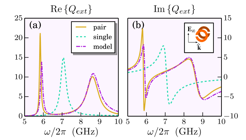
Figure 9: (Color online) The (a) real and (b) imaginary parts of the complex extinction spectrum for a broadside-coupled pair of SRRs, comparing the model with the directly calculated results. For reference, the extinction of a single SRR is also shown. The inset gives the polarization of the incident wave.

It can be seen that the model gives very good agreement with the direct calculation. This agreement can be improved by considering more than one mode on each of the rings. The dominant mode of each ring is mode 1 shown in Fig. 4(b). It is clear from inspection of mode 2 that it has quite different symmetry to mode 1, and it was confirmed numerically that it does not play a role in coupling between rings in this configuration. However, mode 3 also has opposite signs of the charges across the SRR gap just like mode 1, and it also plays a role in the formation of the modes of the coupled system. This is illustrated in Fig. 10, which gives a magnified view of the lower frequency hybridized mode. It can be seen that the additional mode further increases the accuracy of the model, and clearly indicates the contribution of this mode to the coupling process. It was found that the remaining discrepancy is not remedied by increasing the number of modes in the coupled model. Instead, it is due to the impedance of the single ring being fitted near its resonance, whereas the resonances of the coupled system are strongly shifted, to a region where the fitting is less accurate. Improved accuracy would require a robust approach to fit a higher-order model than Eq. (8) to the data, and the frequency dependence of the current eigenvector $I^{(\alpha)}$ to be accounted for, which have not been achieved so far. However, the accuracy of the existing approach is likely to be sufficient for most applications, even if only the dominant mode is considered.

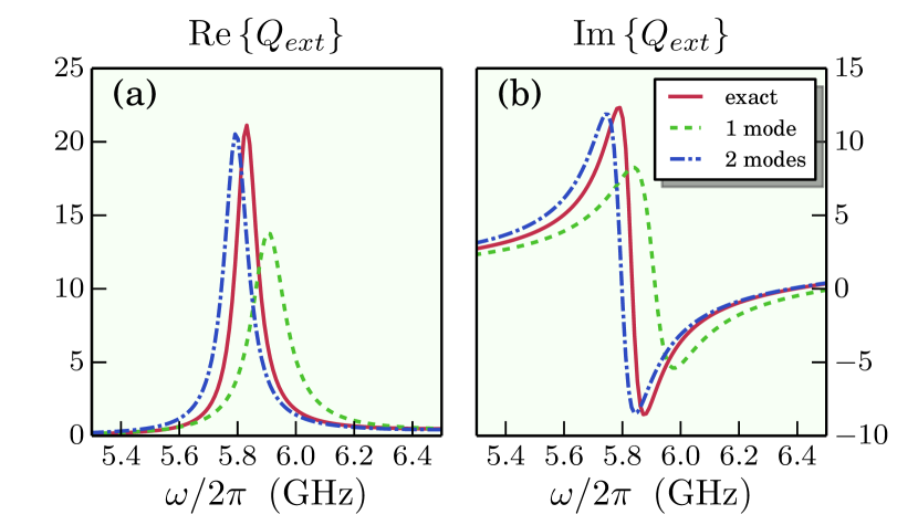
Figure 10: (Color online) Improved accuracy of the model of a broadside-coupled SRR when including an additional mode in the calculation. Comparing the (a) real part and (b) imaginary part of the models against the direct calculation.

V Conclusion

In this paper, a technique was presented to describe the physics of meta-atoms, (nano-)antennas and similar small resonant particles. Using an integral operator approach allows the radiation boundary conditions to be modeled efficiently, and the modes of the system are found by searching for the complex frequencies where this operator becomes singular. It was shown that this approach remains physically meaningful and accurate in regimes where dipole and quasi-static models fail. The coupling of two rings to form a broadside-coupled SRR was studied, showing that the coupling coefficients are smooth, and can be calculated efficiently. The calculated interaction constants were shown to model not only the frequency splitting, but also the enhancement and suppression of radiation losses for the two modes of the coupled system. It was demonstrated that the model can readily incorporate higher-order corrections due to additional modes of each scatterer contributing to the coupled mode.

Appendix A Details of the EFIE

The free space Green’s function appearing in the electric field integral equation is given by

$$\overline{\overline{G}}_{0}\left(\mathbf{r}\right)=\left[-s\mu\overline{\overline{I}}+\frac{1}{s\epsilon}\nabla\nabla\right]\frac{\exp(-\gamma|\mathbf{r}|)}{4\pi|\mathbf{r}|}.$$ (12)

The electric field integral equation is tested and weighted to obtain the impedance matrix $\mathrm{Z}(s)$. After algebraic manipulation to transfer the gradient operations onto the basis functions, the elements of the impedance matrix are given by Gibson (2008)

$$Z_{mn}=\iint_{T_{m}}\iint_{T_{n}}\left(s\mu\mathbf{f}_{m}\left(\mathbf{r}\right)\cdot\mathbf{f}_{n}\left(\mathbf{r}^{\prime}\right)+\frac{1}{s\varepsilon}\left[\nabla\cdot\mathbf{f}_{m}\left(\mathbf{r}\right)\right]\left[\nabla^{\prime}\cdot\mathbf{f}_{n}\left(\mathbf{r}^{\prime}\right)\right]\right)\frac{e^{-\gamma\left|\mathbf{r}-\mathbf{r^{\prime}}\right|}}{4\pi\left|\mathbf{r}-\mathbf{r^{\prime}}\right|}\mathrm{d^{2}}\mathbf{r}^{\prime}\mathrm{d}^{2}\mathbf{r},$$ (13)

where $\varepsilon$ and $\mu$ are the permittivity and permeability of the background medium.

Appendix B Implementation details

The approach proposed in this paper is implemented in an open source code ope . Some essential details of the numerical techniques and computational tools used are given here. The geometry is created in boundary representation (B-rep) form, and is converted to a triangular surface mesh using the package gmsh Geuzaine and Remacle (2009). Basis functions are then defined on the mesh, using either rooftops Rao et al. (1982), or loops and stars Vecchi (1999), which give superior spectral properties for mesh elements which are small compared to the wavelength.

The singularities of Eq. (13) as $\mathbf{r}\rightarrow\mathbf{r}^{\prime}$ are integrable, and are accounted for by subtracting the singular terms from the Green’s function and integrating them separately Arcioni et al. (1997); Hanninen et al. (2006). The remaining non-singular integrals are computed using a fifth order symmetric integration rule Dunavant (1985).

The oscillator model given by Eq. (8) is fitted using the non-negative least squares algorithm, which ensures that only real coefficients of the correct sign appear in the fitting polynomial Lawson and Hanson (1995). The result is a fitted impedance function where the real part is positive to satisfy passivity, and the imaginary part increase with frequency in accordance with Foster’s reactance theorem Foster (1924).

The code to implement these methods is written in the Python language, with the most computationally intensive routines written in Fortran. It utilizes the scientific python tools numpy, scipy, matplotlib and IPython. Perez and Granger (2007); Hunter (2007); Oliphant (2007); Peterson (2009).

Appendix C Search procedure for resonances

Finding the zeros of $\mathrm{Z}(s)$ involves the solution of a transcendental equation, and it is necessary to use iterative techniques. The iterative search uses Newton iteration to find the value of $s$ which minimizes the functional Ruhe (1973)

$$F(s)=\frac{\mathrm{I}(s)\cdot\mathrm{Z}(s)\cdot\mathrm{I}(s)}{\mathrm{I}(s)\cdot\left[\frac{\mathrm{d}}{\mathrm{d}s}\mathrm{Z}(s)\right]\cdot\mathrm{I}(s)}.$$

The functional is evaluated numerically, with the derivatives of $\mathrm{Z}$ approximated by the difference between subsequent iterations.

A key requirement for successful application of iterative methods is a good initial guess, and the approach presented here was empirically found to be robust. The first step is to decompose the impedance matrix, as per Eq. 4. These matrices are evaluated at some arbitrary initial frequency $s_{i}$, and the linearized problem is obtained by neglecting frequency variation of these matrices and solving for the homogeneous solutions $\tilde{s}^{(l)}$ and $\tilde{\mathrm{I}}^{(l)}$ of

$$\mathrm{S}\left(s_{i}\right)\cdot\tilde{\mathrm{I}}^{(l)}=-\left(\tilde{s}^{(l)}\right)^{2}\mathrm{L}\left(s_{i}\right)\cdot\tilde{\mathrm{I}}^{(l)},$$ (14)

which is a generalized eigenvalue problem solvable by standard routines. However, Eq. (14) has non-physical solution at $s=0$ corresponding to the null space of the scalar potential part of the impedance operator. These solutions can be eliminated through the use of loop-star basis functions, which decompose the current into loops (having zero divergence) and stars (the remaining component which is almost irrotational) Vecchi (1999). Each vector and matrix is partitioned between loop ($\mathrm{l}$) and star ($\mathrm{s}$) components, where by the zero divergence of the loop basis functions, Eq. (14) becomes:

$$\begin{bmatrix}0&0\\ 0&\mathrm{S_{ss}}\end{bmatrix}\begin{bmatrix}\tilde{\mathrm{I}}_{\mathrm{l}}\\ \tilde{\mathrm{I}}_{\mathrm{s}}\end{bmatrix}=-\left(\tilde{s}^{(l)}\right)^{2}\begin{bmatrix}\mathrm{L_{ll}}&\mathrm{L_{ls}}\\ \mathrm{L_{sl}}&\mathrm{L_{ss}}\end{bmatrix}\begin{bmatrix}\tilde{\mathrm{I}}_{\mathrm{l}}\\ \tilde{\mathrm{I}}_{\mathrm{s}}\end{bmatrix}.$$ (15)

First note that for $s=0$, any solution with $\tilde{\mathrm{I}}_{\mathrm{s}}=0$ will satisfy this equation. These are the solutions to be eliminated, whereas for the cases of physical interest $\tilde{\mathrm{I}}_{\mathrm{l}}=-\mathrm{L_{ll}}^{-1}\mathrm{L_{ls}\tilde{\mathrm{I}}_{s}}$. This leads to the eigenvalue problem

$$\mathrm{S_{ss}}\tilde{\mathrm{I}}_{\mathrm{s}}=-\left(\tilde{s}^{(l)}\right)^{2}\left[\mathrm{L_{ss}}-\mathrm{L_{ls}\mathrm{L_{ll}}^{-1}L_{ls}}\right]\tilde{\mathrm{I}}_{\mathrm{s}},$$

which is solved to find the trial solution $\tilde{\mathrm{I}}_{\mathrm{s}}$ and $\tilde{s}^{(l)}$, used to start the Newton iteration procedureRuhe (1973); Lancaster (1966).

References

- Simovski (2011) C. R. Simovski, J. Opt. 13, 013001 (2011).
- Zeng et al. (2012) Y. Zeng, D. A. Dalvit, J. O’Hara, and S. Trugman, Phys. Rev. B 85, 1 (2012).
- (3) “OpenModes: An eigenmode solver for open electromagnetic resonantors,” Available at http://pythonhosted.org/OpenModes/.
- Alonso-Gonzalez et al. (2011) P. Alonso-Gonzalez, M. Schnell, P. Sarriugarte, H. Sobhani, C. Wu, N. Arju, A. B. Khanikaev, F. Golmar, P. Albella, L. Arzubiaga, F. Casanova, L. E. Hueso, P. Nordlander, G. Shvets, and R. Hillenbrand, Nano Lett. 11, 3922 (2011).
- Miroshnichenko et al. (2010) A. Miroshnichenko, S. Flach, and Y. S. Kivshar, Rev. Mod. Phys. 82, 2257 (2010).
- Bilotti et al. (2007) F. Bilotti, A. Toscano, L. Vegni, K. Aydin, K. B. Alici, and E. Ozbay, IEEE Trans. Microw. Theory Tech. 55, 2865 (2007).
- Ikonen and Tretyakov (2007) P. M. T. Ikonen and S. A. Tretyakov, IEEE Trans. Microw. Theory Tech. 55, 92 (2007).
- Karyamapudi (2005) B. Karyamapudi, IEEE Microw. Wirel. Components Lett. 15, 706 (2005).
- Staffaroni et al. (2012) M. Staffaroni, J. Conway, S. Vedantam, J. Tang, and E. Yablonovitch, Photonics Nanostructures - Fundam. Appl. 10, 166 (2012).
- Sersic et al. (2011) I. Sersic, C. Tuambilangana, T. Kampfrath, and A. F. Koenderink, Phys. Rev. B 83, 245102 (2011).
- Bohren and Huffman (1983a) C. F. Bohren and D. R. Huffman, Absorption and Scattering of Light by Small Particles (John Wiley & Sons, New York, 1983).
- Krasnok et al. (2014) A. Krasnok, C. Simovski, P. Belov, and Y. S. Kivshar, Nanoscale 6, 7354 (2014).
- Mayergoyz et al. (2005) I. Mayergoyz, D. Fredkin, and Z. Zhang, Phys. Rev. B 72, 155412 (2005).
- Davis et al. (2009) T. Davis, K. Vernon, and D. Gómez, Phys. Rev. B 79, 155423 (2009).
- Yakovlev and Hanson (2000) A. B. Yakovlev and G. Hanson, IEEE Trans. Microw. Theory Tech. 48, 67 (2000).
- Davoyan et al. (2010) A. Davoyan, I. V. Shadrivov, S. I. Bozhevolnyi, and Y. S. Kivshar, J. Nanophotonics 4, 043509 (2010).
- Viviescas and Hackenbroich (2003) C. Viviescas and G. Hackenbroich, Phys. Rev. A 67, 013805 (2003).
- Jenkins and Ruostekoski (2012) S. D. Jenkins and J. Ruostekoski, Phys. Rev. B 86, 085116 (2012).
- Leung et al. (1994) P. Leung, S. Liu, and K. Young, Phys. Rev. A 49, 3057 (1994).
- Kristensen et al. (2012) P. T. Kristensen, C. Van Vlack, and S. Hughes, Opt. Lett. 37, 1649 (2012).
- Sauvan et al. (2013) C. Sauvan, J. P. Hugonin, I. S. Maksymov, and P. Lalanne, Phys. Rev. Lett. 110, 237401 (2013).
- Bai et al. (2013) Q. Bai, M. Perrin, C. Sauvan, J.-P. Hugonin, and P. Lalanne, Opt. Express 21, 27371 (2013).
- Hanson and Yakovlev (2002) G. W. Hanson and A. B. Yakovlev, Operator Theory for Electromagnetics (Springer-Verlag, New York, NY, 2002).
- Kovalyov and Ponomarev (2011) I. P. Kovalyov and D. M. Ponomarev, IEEE Trans. Antennas Propag. 59, 4181 (2011).
- Shestopalov and Shestopalov (1996) V. P. Shestopalov and Y. V. Shestopalov, Spectral theory and excitation of open structures (The Institution of Electrical Engineers, London, 1996).
- Harrington (1968) R. F. Harrington, Field Computation by Moment Methods (Macmillan, New York, 1968).
- Gibson (2008) W. C. Gibson, The Method of Moments in Electromagnetics (Chapman & Hall/CRC, Boca Raton, 2008).
- Kern and Martin (2009) A. M. Kern and O. J. Martin, J. Opt. Soc. Am. A 26, 732 (2009).
- Ergül (2012) O. Ergül, J. Opt. 14, 062701 (2012).
- Zheng et al. (2013a) X. Zheng, N. Verellen, V. Volskiy, V. K. Valev, J. J. Baumberg, G. A. E. Vandenbosch, and V. V. Moshchalkov, Opt. Express 21, 31105 (2013a).
- Greffet et al. (2010) J.-J. Greffet, M. Laroche, and F. Marquier, Phys. Rev. Lett. 105, 117701 (2010).
- Glisson et al. (1983) A. Glisson, D. Kajfez, and J. James, IEEE Trans. Microw. Theory Tech. 31, 1023 (1983).
- Baum (1976) C. E. Baum, Proc. IEEE 64, 1598 (1976).
- Baum (1978) C. E. Baum, in Electromagnetic Scattering, edited by P. L. E. Uslenghi (1978) Chap. 15, pp. 571–651.
- Mäkitalo et al. (2014) J. Mäkitalo, M. Kauranen, and S. Suuriniemi, Phys. Rev. B 89, 165429 (2014).
- Zheng et al. (2013b) X. Zheng, V. Volskiy, V. Valev, G. Vandenbosch, and V. Moshchalkov, IEEE J. Quant. Electron. 19, 4600908 (2013b).
- Ylä-Oijala et al. (2005) P. Ylä-Oijala, M. Taskinen, and S. Järvenpää, Radio Sci. 40, 1 (2005).
- Michalski and Mosig (1997) K. Michalski and J. R. Mosig, IEEE Trans. Antennas Propag. 45, 508 (1997).
- Simovski and Tretyakov (2010) C. R. Simovski and S. A. Tretyakov, Photonics Nanostructures - Fundam. Appl. 8, 254 (2010).
- Kennelly (1936) A. Kennelly, Electr. Eng. J. Inst. , 235 (1936).
- Bekers et al. (2009) D. J. Bekers, S. van Eijndhoven, and A. G. Tijhuis, IEEE Trans. Antennas Propag. 57, 3772 (2009).
- Hopkins et al. (2013) B. Hopkins, A. N. Poddubny, A. E. Miroshnichenko, and Y. S. Kivshar, Phys. Rev. A 88, 053819 (2013).
- Marin (1973) L. Marin, IEEE Trans. Antennas Propagat. 21, 809 (1973).
- Andrew et al. (1993) A. L. Andrew, K.-W. E. Chu, and P. Lancaster, SIAM J. Matrix Anal. Appl. 14, 903 (1993).
- Baum (1975) C. E. Baum, Interaction Note 229: On the Eigenmode Expansion for Electromagnetic Scattering and Antenna Problems, Part I: Some Basic Relations for Eigenmode Expansions and Their Relation to the Singularity Expansions, Tech. Rep. (1975).
- Note (1) The enclosing sphere is used rather than the more common geometric cross-section of the object, since the geometric cross-section can be very small for certain cases such as thin-wire metamaterials.
- Bohren and Huffman (1983b) C. F. Bohren and D. R. Huffman, Absorption and Scattering of Light by Small Particles (John Wiley & Sons, New York, 1983).
- Vandenbosch (2010) G. A. E. Vandenbosch, IEEE Trans. Antennas Propag. 58, 1112 (2010).
- Prodan et al. (2003) E. Prodan, C. Radloff, N. J. Halas, and P. Nordlander, Science 302, 419 (2003).
- Liu et al. (2007) H. Liu, D. Genov, D. Wu, Y. Liu, Z. Liu, C. Sun, S. Zhu, and X. Zhang, Phys. Rev. B 76, 073101 (2007).
- Powell et al. (2011) D. A. Powell, K. E. Hannam, I. V. Shadrivov, and Y. S. Kivshar, Phys. Rev. B 83, 235420 (2011).
- Powell et al. (2010) D. A. Powell, M. Lapine, M. V. Gorkunov, I. V. Shadrivov, and Y. S. Kivshar, Phys. Rev. B 82, 155128 (2010).
- Decker et al. (2011) M. Decker, N. Feth, C. M. Soukoulis, S. Linden, and M. Wegener, Phys. Rev. B 84, 085416 (2011).
- Turner et al. (2010) M. D. Turner, M. M. Hossain, and M. Gu, New J. Phys. 12, 083062 (2010).
- Liu et al. (2012) M. Liu, D. A. Powell, I. V. Shadrivov, and Y. S. Kivshar, Appl. Phys. Lett. 100, 111114 (2012).
- Tatartschuk et al. (2012) E. Tatartschuk, N. Gneiding, F. Hesmer, A. Radkovskaya, and E. Shamonina, J. Appl. Phys. 111, 094904 (2012).
- Marqués et al. (2002) R. Marqués, F. Medina, and R. Rafii-El-Idrissi, Phys. Rev. B 65, 144440 (2002).
- Geuzaine and Remacle (2009) C. Geuzaine and J.-F. Remacle, Int. J. Numer. Methods Eng. 79, 1309 (2009).
- Rao et al. (1982) S. Rao, D. R. Wilton, and A. Glisson, IEEE Trans. Antennas Propag. 30, 409 (1982).
- Vecchi (1999) G. Vecchi, IEEE Trans. Antennas Propag. 47, 339 (1999).
- Arcioni et al. (1997) P. Arcioni, M. Bressan, and L. Perregrini, IEEE Trans. Microw. Theory Tech. 45, 436 (1997).
- Hanninen et al. (2006) I. Hanninen, M. Taskinen, and J. Sarvas, Prog. Electromagn. Res. 63, 243 (2006).
- Dunavant (1985) D. A. Dunavant, Int. J Numer. Meth. Eng. 21, 1129 (1985).
- Lawson and Hanson (1995) C. L. Lawson and R. J. Hanson, Solving least squares problems (Society for Industrial and Applied Mathematics, Philadelphia, Pa., 1995).
- Foster (1924) R. M. Foster, Bell Syst. Tech. J. 3, 259 (1924).
- Perez and Granger (2007) F. Perez and B. E. Granger, Comput. Sci. Eng. 9, 21 (2007).
- Hunter (2007) J. D. Hunter, Comput. Sci. Eng. 9, 90 (2007).
- Oliphant (2007) T. E. Oliphant, Comput. Sci. Eng. 9, 10 (2007).
- Peterson (2009) P. Peterson, Int. J. Comput. Sci. Eng. 4, 296 (2009).
- Ruhe (1973) A. Ruhe, SIAM J. Numer. Anal. 10, 674 (1973).
- Lancaster (1966) P. Lancaster, Lambda Matrices and Vibrating Systems (Pergamon, Oxford, 1966).