Chaotic zones around gravitating binaries

Abstract

The extent of the continuous zone of chaotic orbits of a small-mass tertiary around a system of two gravitationally bound primaries of comparable masses (a binary star, a binary black hole, a binary asteroid, etc.) is estimated analytically, as a function of the tertiary’s orbital eccentricity. The separatrix map theory is used to demonstrate that the central continuous chaos zone emerges (above a threshold in the primaries’ mass ratio) due to overlapping of the orbital resonances corresponding to the integer ratios $p$:1 between the tertiary and the central binary periods. In this zone, the unlimited chaotic orbital diffusion of the tertiary takes place, up to its ejection from the system. The primaries’ mass ratio, above which such a chaotic zone is universally present at all initial eccentricities of the tertiary, is estimated. The diversity of the observed orbital configurations of biplanetary and circumbinary exosystems is shown to be in accord with the existence of the primaries’ mass parameter threshold.

Key words: binaries: general – planets and satellites: dynamical evolution and stability – planets and satellites: formation – planets and satellites: individual (Kepler-16b)

1 Introduction

Zones of orbital instability are known to exist around binary stars. In particular, such zones are known to be present in circumbinary protoplanetary disks. The latter may contain planetesimals, dust, and gas. Gas is present on the initial stages of the disk evolution; it dissipates later on. Many recent numerical simulations show that, irrespective of the gas content, a free-from-matter central cavity always forms around a system of two gravitationally bound bodies of comparable masses; see (Moriwaki & Nakagawa, 2004; Pierens & Nelson, 2007, 2008; Meschiari, 2012; Paardekooper et al., 2012) for planetesimal disks with and without gas.

The existence and possible characteristics of central cavities in gaseous circumbinary disks were considered theoretically as early as 1994 by Artymowicz & Lubow (1994, 1996), in view of the observational data on the disks around such stars as GW Ori. Artymowicz and Lubow outlined the role of Lindblad resonances in the cavities formation, the cavity size increasing with decreasing the disk viscosity (see, e.g., Figure 4 in Artymowicz & Lubow 1996).

In a quite separate field of study, namely, the dynamical studies of triple stars, it is well known that the stability of hierarchical triple stars is mostly determined by the pericentric distance of the tertiary (Mikkola, 2008; Valtonen et al., 2008; Saito et al., 2012, 2013): if this distance is below a critical one, the system is unstable. A number of heuristic semi-analytical criteria for the critical pericentric distance were proposed (see reviews in Mikkola 2008; Valtonen et al. 2008). Most of these criteria do not appeal to resonant phenomena, with a few exceptions. Mudryk & Wu (2006) explored the overlapping of subresonances of mean motion resonances, which is responsible for defining the local stability borders in the phase space of motion of a planet orbiting a binary, and derived expressions for the subresonance borders. In the general three-body problem, the role of overlap of orbital resonances for the stability of triples was considered by Mardling (2008), who developed an algorithm for constructing the analytical stability border as an envelope of a set of local resonance borders. For the hierarchical triples, Mardling revealed the major role (for the formation of the global stability border) of overlapping of the orbital resonances, corresponding to the integer ratios $p$:1 between the tertiary and the binary periods.

On the other hand, numerical-experimental criteria are of great value (due to their high comparative accuracy) and are mostly used nowadays in studies of the stability of planets in binary systems, especially, in the dynamical studies of circumbinary planets. Holman & Wiegert (1999) derived a numerical-experimental criterion for the radius of the central chaotic zone, in the framework of the planar restricted three-body problem. The observational data on the recently discovered exoplanets orbiting around main-sequence binaries (Kepler-16b, 34b, 35b, and others), combined with estimates based on the Holman–Wiegert criterion, shows that these circumbinary planets move in orbits encircling the central chaotic zone, and usually these orbits are close to its boundary (Doyle et al., 2011; Welsh et al., 2012, 2014; Popova & Shevchenko, 2013).

Nowadays, the circumbinary dynamics is studied mostly in the exoplanetary context. However, the presence of a central chaotic zone is, of course, universal for the dynamics around any gravitating binary with comparable component masses (a binary star, a binary black hole, a binary asteroid, etc.).

In this paper, the extent of the continuous zone of chaotic orbits of a small-mass tertiary around a system of two gravitationally bound bodies of comparable masses is estimated strictly analytically (i.e., without introducing any empirical or heuristic factors). The binary’s mass ratio, above which such a chaotic zone is universally present, is also estimated. Chirikov’s resonance overlap criterion (Chirikov, 1959, 1979) and the general separatrix map theory (Shevchenko, 2007, 2010, 2011) are used. The analysis is performed in the framework of the planar restricted circular three-body problem, i.e., the eccentricity of the central binary is zero, and the orbit of the test zero-mass particle is coplanar with that of the binary.

The paper is organized as follows. In Section 2, we briefly review the existing relevant criteria for the orbital stability of three-body systems, then we consider the separatrix map theory and, based on it, derive a new, strictly analytical criterion for the appearance of a circumbinary zone of the tertiary’s chaotic orbits. In Section 3, using the derived criterion, we estimate the typical size of the circumbinary chaotic zone. It is demonstrated that the central continuous chaos zone emerges due to overlapping of the orbital resonances corresponding to the integer ratios $p$:1 between the tertiary and the central binary periods. In Section 4, we consider a mass parameter threshold, above which the central chaotic zone is universally present at all initial eccentricities of the tertiary. In Section 5, we analyze the theoretical chaos border in a “pericentric distance–eccentricity” stability diagram for exosystem Kepler-16 (the prototype of circumbinary exosystems), and inspect how well the theoretical border fits the numerical-experimental one. In Section 6, we discuss the relevance of the mass parameter threshold to the diversity of the observed orbital configurations of biplanetary and circumbinary exosystems. Section 7 is devoted to our conclusions.

2 An analytical criterion based on the Kepler map

First of all, let us recall the case in which the masses of the binary components are not comparable, i.e., one of them is much less than the other one. Then, as shown by Wisdom (1980), a narrow annular chaotic band exists, surrounding the orbit of the secondary. The inner half-band forms due to accumulation of the first-order resonances $(p+1)$:$p$ between the orbital periods of the secondary and the tertiary, and the outer one forms due to the accumulation of the resonances $p$:$(p+1)$ between the same periods. With increasing $p$, the resonances group more densely, and, at some threshold value of $p$, they start to overlap because the resonance width does not shrink fast enough with $p$. Chirikov’s resonance overlap criterion states that when resonances overlap, global chaos emerges (Chirikov, 1959, 1979; Lichtenberg & Lieberman, 1992). On these grounds, Wisdom (1980) showed, in the framework of the planar circular restricted three-body problem, that in the case of small eccentricity ($e\lesssim 0.15$) of the particle’s orbit, the value of $p$, critical for the overlap of the first-order resonances, is given by

$$p_{\mathrm{overlap}}\approx 0.51\mu^{-2/7},$$ (1)

where $\mu=m_{2}/(m_{1}+m_{2})$ is the mass parameter of the binary; $\mu\ll 1$. Let $a$ and $a^{\prime}$ be the semimajor axes of the particle’s and perturber orbits, respectively; then, using Equation (1) and Kepler’s third law, it is straightforward to find the interval $\Delta a_{\mathrm{overlap}}=|a-a^{\prime}|$, where the $(p+1)$:$p$ resonances overlap:

$$\Delta a_{\mathrm{overlap}}\approx 1.3\mu^{2/7}a^{\prime}$$ (2)

(Duncan et al., 1989; Murray & Dermott, 1999). The particles with $a\in a^{\prime}\pm\Delta a_{\mathrm{overlap}}$ move chaotically. Thus, the radial extent of the instability neighborhood of the perturber’s orbit is given by the “$\mu^{2/7}$ law”.

Murray & Dermott (1999) checked the validity of this analytical result in direct numerical integrations of orbits. It turned out that in a studied interval of $\mu$ (which was rather broad: $10^{-9}\leq\mu\leq 10^{-3}$) the numerically derived power-law index is equal to $0.286$, practically coinciding with the theoretical prediction $2/7$, but the coefficient $1.3$ is in fact $\sim 30\%$ greater:

$$\Delta a_{\mathrm{overlap}}=1.57\mu^{0.286}a^{\prime}$$ (3)

(see Figure 9.23 in Murray & Dermott 1999). This means that the real chaotic annular zone is about $30\%$ broader, regardless of the $\mu$ value.

Formally extrapolating Equation (3) to $\mu=1/2$ (the equal-mass case), one finds $\Delta a_{\mathrm{overlap}}/a^{\prime}\approx 1.29$, i.e., the zone inside the binary is expected to be continuously chaotic, and the outer border of this continuous chaotic zone is expected to be situated at $\approx(0.5+1.29)a^{\prime}\approx 1.8a^{\prime}$ from the barycenter (the binary’s center of mass). We shall see that this severely underestimates the actual size (in fact, the actual size $\approx 2.8a^{\prime}$). The reason for the discrepancy is not just a numerical uncertainty of extrapolation. It is deeply physical: as we shall see, the class of resonances responsible for the formation of the central chaotic zone is totally different from that responsible for the formation of the annular chaotic band.

As massive numerical data show (see Holman & Wiegert 1999; Valtonen et al. 2008), when the binary’s components are comparable in mass, the central continuous chaotic zone indeed exists. The zone size depends, in particular, on the tertiaries’ initial eccentricities (Valtonen et al., 2008); if they are zero, then the size can be estimated (in the planar restricted three-body problem) using the Holman–Wiegert numerical-experimental criterion (Holman & Wiegert, 1999): the radius $a_{\mathrm{cr}}$ of the instability zone for the initially circular prograde circumbinary orbits is given by the smooth fitting function

$$a_{\mathrm{cr}}/a_{\mathrm{b}}=1.60+5.10e_{\mathrm{b}}-2.22e_{\mathrm{b}}^{2}+4.12\mu-4.27e_{\mathrm{b}}\mu-5.09\mu^{2}+4.61e_{\mathrm{b}}^{2}\mu^{2},$$ (4)

where $\mu=m_{2}/(m_{1}+m_{2})$, and $a_{\mathrm{b}}$ and $e_{\mathrm{b}}$ are the semimajor axis and eccentricity of the binary. Thus, the Holman–Wiegert criterion, Equation (4), utilizes a polynomial fit over numerical data in $a_{\mathrm{b}}$ and $e_{\mathrm{b}}$ for the description of the global instability border location. However, note that this border is in fact fractal (Popova & Shevchenko, 2012, 2013); an example of its “ragged” appearance will be given below.

In what follows, we analytically explore the phenomenon of the circumbinary chaos zone. Similarly to the above-mentioned accumulation of the first-order resonances $(p+1)$:$p$ in the close-to-coorbital motion, there exists an accumulation of resonances $p$:1 in the circumbinary highly eccentric motion, close to the parabolic one.

To describe this accumulation of resonances, we use the “Kepler map” theory, initiated by Petrosky (1986), Petrosky & Broucke (1988) and Chirikov & Vecheslavov (1986). They found that if one writes down the expression for the tertiary’s energy $E$ increment together with the expression for the time increment between two consecutive pericenter passages by the tertiary (this time increment is directly proportional to the increment of perturber’s phase angle $g$, and is expressed through the energy via Kepler’s third law), one obtains a two-dimensional area-preserving map, the so-called Kepler map:

$$E_{i+1} = E_{i}+W\sin g_{i},$$

$$g_{i+1} = g_{i}+2\pi|2E_{i+1}|^{-3/2},$$ (5)

where the subscript $i$ enumerates the pericenter passages. (On the general theory of area-preserving maps, see Meiss 1992.) As derived in Shevchenko (2011), in the case of prograde (with respect to the binary) tertiary orbits, the coefficient $W$ is given by

$$W\simeq 2^{1/4}\pi^{1/2}\mu q^{-1/4}\exp\left(-\frac{2^{3/2}q^{3/2}}{3}\right),$$ (6)

if $\mu\ll 1/2$ and $q=a(1-e)>1$ ($q$ is the tertiary’s pericentric distance). Hereafter we set the gravitational constant $G=1$, the sum of the masses of the binary’s components $m_{1}+m_{2}=1$, and the binary’s semimajor axis $a_{\mathrm{b}}=1$ (then the binary’s period is equal to $2\pi$).

By means of substitution $E=Wy$, $g=x$, map (5) is reducible to

$$y_{i+1} = y_{i}+\sin x_{i},$$

$$x_{i+1} = x_{i}+\lambda|y_{i+1}|^{-3/2},$$ (7)

where

$$\lambda=2^{-1/2}\pi W^{-3/2}.$$ (8)

Thus, the Kepler map is parameterized by the single parameter $\lambda$ (Shevchenko, 2010). Both maps (5) and (7) depend on a single parameter, be it $\lambda$ or $W$, but the advantage of Equations (7) over (5) is that the $\lambda$ parameter in Equations (7) is an analog of the adiabaticity parameter in the case of the classical separatrix map (derived in Chirikov 1979); therefore, by its value, one can judge whether chaos is adiabatic or not. (The term “adiabatic chaos” concerns the conservation of an adiabatic invariant; at low values of $\lambda$, it is conserved on long time intervals between crossings of the separatrix, see Chirikov & Vecheslavov 2000; Shevchenko 2008.)

The Kepler map is an example of a general separatrix map (Shevchenko, 2010), the separatrix (the $y=0$ line) separating the bound and unbound states of the particle’s motion. At $q\gg 1$, one has $W\ll 1$ (see Equation (6)), therefore $\lambda\gg 1$. This means that chaos in the motion of particles is not adiabatic (Shevchenko, 2007), and therefore the Kepler map can be locally approximated by the standard map with good accuracy (Shevchenko, 2010, 2011).

The Kepler map is derived in the assumption that the tertiary’s pericentric distance $q$ is constant. This can be justified quite easily, using the classical Tisserand relation (based on the Jacobi constant formalism). In the planar circular restricted three-body problem, the Tisserand relation is given by

$$\frac{1}{a}+2\left[(1-e^{2})a\right]^{1/2}\approx\mathrm{const},$$ (9)

where $a$ is the semimajor axis of the particle, measured in the units of the perturber’s semimajor axis $a^{\prime}$, $e$ is the particle’s eccentricity (see, e.g., Murray & Dermott 1999). If $a\gg a^{\prime}$, and $e\sim 1$, one has

$$\frac{1}{a}+2\left[(1+e)q\right]^{1/2}\approx 2^{3/2}q^{1/2}\approx\mathrm{const}.$$ (10)

Thus, $q$ is approximately conserved.

Petrosky (1986) used the Kepler map theory to show that the energy width of a one-sided chaotic band in the vicinity of the perturbed parabolic orbit scales as the power $2/5$ of the mass parameter:

$$\Delta E_{\mathrm{cr}}=\left|E_{\mathrm{cr}}\right|=-E_{\mathrm{cr}}\propto\mu^{2/5},$$ (11)

if $\mu\ll 1$. The particles with $E\in(-\Delta E_{\mathrm{cr}},0)$ move chaotically. Thus, Equation (11) represents the “$\mu^{2/5}$ law”.

It is interesting that the power-law index in the scaling $r_{\mathrm{H}}\propto\mu^{1/3}$ for the radius of the regular zone (the Hill sphere, see Murray & Dermott 1999) around the secondary is intermediate between the indices in the Wisdom and “Kepler-map” scalings, given by Equations (2) and (11), respectively. Thus, the indices form a sequence: 2/5, 2/6, 2/7.

Let us characterize the size of the central continuous chaotic zone in the space of orbital elements. Linearizing the Kepler map (7) in $y$ near the fixed point at the border of the map’s chaotic layer (thus, the Kepler map is locally approximated by the standard map, which is a mathematical model of a multiplet of equally spaced and equally sized resonances, see Shevchenko 2014), one finds for the location of the border:

$$y_{\mathrm{cr}}=\left(\frac{3\lambda}{2K_{G}}\right)^{2/5},$$ (12)

where $K_{G}=0.971635406\dots$ (Shevchenko, 2007). Using Equations (6) and (8) for $W$ and $\lambda$, one arrives at

$$\Delta E_{\mathrm{cr}}=\left|E_{\mathrm{cr}}\right|=\left|Wy_{\mathrm{cr}}\right|\simeq A\mu^{2/5}q^{-1/10}\exp\left(-Bq^{3/2}\right),$$ (13)

where

$$A=2^{-1/2}3^{2/5}\pi^{3/5}K_{G}^{-2/5}=2.2061\dots,\qquad B=2^{5/2}/15=0.3771\dots.$$

The particle’s critical eccentricity $e_{\mathrm{cr}}$, following from the relation $\Delta E_{\mathrm{cr}}=-E_{\mathrm{cr}}=1/(2a_{\mathrm{cr}})=(1-e_{\mathrm{cr}})/(2q)$, is

$$e_{\mathrm{cr}}=1-2q\Delta E_{\mathrm{cr}},$$ (14)

where $\Delta E_{\mathrm{cr}}$ is given by Equation (13). The orbits with $e\gtrsim e_{\mathrm{cr}}(q)$ are chaotic.

What if $\mu\approx 1/2$, i.e., the binary is approximately equal-mass? This is quite common in stellar binaries. According to (Roy & Haddow, 2003, formula (26)), the energy increment in the $\mu=1/2$ case in the restricted problem limit is given by

$$\delta E\simeq-2^{7/4}\pi^{1/2}q^{3/4}\exp\left(-\frac{2^{5/2}q^{3/2}}{3}\right)\sin 2g_{i}.$$ (15)

The possibility to use the Kepler map at moderate and high values of $\mu$ (i.e., at $\mu\sim 1/2$) was discussed in Shevchenko (2010). Note that, in Equations (5), the harmonic term in the first line ($\propto\sin g_{i}$) is just the first most prominent one in the Fourier expansion of the energy increment, if $\mu\ll 1$ (Petrosky, 1986; Shevchenko, 2011). If one increases $\mu$, the second harmonic ($\propto\sin 2g_{i}$) becomes more and more important. If $\mu=1/2$, the first harmonic ($\propto\sin g_{i}$) disappears, whereas the second one ($\propto\sin 2g_{i}$) becomes largest in the series expansion because, due to the equality of the primaries’ masses, the perturbation frequency is effectively doubled. Thus, the Kepler map, formally, takes the form

$$E_{i+1} = E_{i}+W_{1/2}\sin 2g_{i},$$

$$g_{i+1} = g_{i}+2\pi|2E_{i+1}|^{-3/2},$$ (16)

where

$$W_{1/2}\simeq-2^{7/4}\pi^{1/2}q^{3/4}\exp\left(-\frac{2^{5/2}q^{3/2}}{3}\right).$$ (17)

By means of substitution $E=W_{1/2}y$, $g=x/2$, map (16) is reducible to map (7) with

$$\lambda=2^{1/2}\pi W_{1/2}^{-3/2},$$ (18)

and $y_{\mathrm{cr}}$ is given by Equation (12). Thus, in the $\mu=1/2$ case one has

$$\Delta E_{\mathrm{cr}}=\left|W_{1/2}y_{\mathrm{cr}}\right|\simeq A_{1/2}q^{3/10}\exp\left(-B_{1/2}q^{3/2}\right),$$ (19)

where

$$A_{1/2}=2^{1/2}3^{2/5}\pi^{3/5}K_{G}^{-2/5}=4.4122\dots,\qquad B_{1/2}=2^{7/2}/15=0.7542\dots.$$

The critical eccentricity $e_{\mathrm{cr}}$ is given by formula (14).

As illustrated in the next section, the critical curve given by Equation (19) looks somewhat different from a curve resulting from convergence of the critical curves given by Equation (13) at $\mu\to 1/2$, though the locations of both curves are approximately the same. The difference is due to the fact that the actual energy increment is not given by a single harmonic term, but is a Fourier series of harmonic terms (Petrosky, 1986; Liu & Sun, 1994), from which we have taken only the leading terms: the term $\propto\sin g_{i}$ in the case of $\mu\ll 1$, and the term $\propto\sin 2g_{i}$ in the case of $\mu\approx 1/2$. Taking into account additional harmonic terms is important, in particular, at $q$ close to 1 (see Liu & Sun 1994).

3 Size of the circumbinary chaotic zone

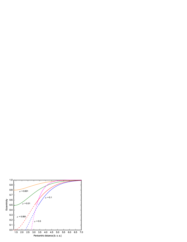
Figure 1: Critical curves, given by Equation (14), for several values of the mass parameter $\mu$. The curves separate chaotic and regular domains (chaos is on the left). Extrapolations are dashed. The pericentric distance is measured in the units of the central binary’s semimajor axis (abbreviated as “b. s. a.” at the horizontal axis caption).

In Figure 1, theoretical dependences “pericentric distance $q$–critical eccentricity $e_{\mathrm{cr}}$”, are constructed for several values of $\mu$, using the formulae derived above. Global chaos extends to the left of the curves. Tentatively extrapolating the critical curves to zero eccentricity, one sees that, if $\mu=0.1$, the curve hits the horizontal axis at $q=2.3$, and, from Kepler’s third law, this corresponds to the ratio $\approx 3.5$ between the orbital periods of the particle and the binary. The value of $q=2.8$ (where the critical curve hits the horizontal axis at $\mu=0.5$) corresponds to the ratio $\approx 4.7$. Thus, the extrapolation of the critical curve to zero eccentricity gives $q$ rather insensitive to $\mu$ in the range $\mu\sim 0.1$–$0.5$, which is typical for binary stars. If $\mu$ is in this range, the chaotic zone boundary lies in the region of resonances from 7/2 to 5/1.

We extrapolate the curves given by the Kepler map theory to the tertiary’s low eccentricities. To emphasize the extrapolative character of the curves at low eccentricities, they are dashed at $e<0.5$. However, the theory was developed for high eccentricities. The possibility of such an extrapolation is justified post factum: the curves corresponding to $\mu\sim 0.1$–$0.5$ hit the $e=0$ axis at high enough values of $q$, at which the higher-order harmonics in the Fourier expansion of the energy increment are relatively unimportant because these harmonics are exponentially small with the harmonic order $j$ (they are proportional to $\exp(-4jq^{3/2}/(2^{1/2}3))$; Petrosky 1986; Petrosky & Broucke 1988).

Thus, according to the theoretical dependences presented in Figure 1, the central chaotic zone’s radial size, measured in the units of binary’s semimajor axis, is $\sim 3$ at moderate eccentricities, and $\sim 2.3$–2.8 at zero eccentricities of the tertiaries, if one considers primaries of comparable masses ($\mu\sim 0.1$–0.5).

At $e=0$, the estimate can be compared to that given by the numerical-experimental criterion of Holman & Wiegert (1999). Since fit (4) was accomplished in Holman & Wiegert (1999) for $\mu\geq 0.1$, we make comparisons at $\mu\geq 0.1$. Setting $e_{\mathrm{b}}=0$ in Equation (4), for $\mu=0.1$ and $0.5$ one obtains $a_{\mathrm{cr}}/a_{\mathrm{b}}=2.0$ and $2.4$, whereas Figure 1 gives $a_{\mathrm{cr}}/a_{\mathrm{b}}=2.3$ and $2.8$, respectively. The agreement, taking into account the extrapolative character of our predictions and the strongly “ragged” character of the global chaos border at low values of $e$ (see Section 5), can be considered rather good, though a systematic shift is present.

Our results at $e=0$ can be also compared to semianalytical data presented in Szebehely (1980) and Szebehely & McKenzie (1981), who employed computations of the topology of the zero velocity curves in the circular restricted three-body problem in the framework of the Hill–Lyapunov approach. At $\mu=0.1$, $0.24$, and $0.5$, Szebehely (1980) and Szebehely & McKenzie (1981) obtained $a_{\mathrm{cr}}/a_{\mathrm{b}}\approx 2.24$, $2.4$, and $2.17$, whereas, from our formulas, one has $a_{\mathrm{cr}}/a_{\mathrm{b}}\approx 2.29$, $2.91$, and $2.79$, respectively. At $\mu=0.1$ the agreement is perfect, and it is even better than that with the data of Holman & Wiegert (1999), but at $\mu=0.5$ the divergence is rather large. The nature of this divergence needs further analysis. A comparison of the results of Szebehely & McKenzie (1981) with fit (4) is discussed in Holman & Wiegert (1999).

4 The mass parameter threshold

In Figure 1, the theoretical curves start (on increasing $\mu$) to hit the horizontal axis $e=0$ at $\mu\approx 0.0547\sim 0.05$; thus, this value of $\mu$ can be considered as an approximate threshold value at which the central continuous chaotic zone, emerging due to the overlap of the $p$:1 resonances, appears at all eccentricities of the tertiaries. (Note that our analysis solely concerns the circumbinary orbits; for the circumcomponent (satellite-type) orbits, stable orbits always exist inside the Hill spheres of the binary components.)

This threshold has a notable physical meaning: above it, the tertiary, even starting from a small eccentricity, can diffuse, following the sequence of the overlapping $p$:1 resonances, up to ejection from the system; close encounters with other bodies are not required for the escape. Below it, the diffusion in the overlapping $(p+1)$:$p$ resonances does not lead, in itself, to the ejection; the chaotic band surrounding the secondary’s orbit is “cleaned up” due to close encounters of the tertiaries with the secondary.

The prediction for the threshold relies on the mentioned rather sharp transition in the behavior of the extrapolated critical curves, taking place at $\mu\sim 0.05$. The actual threshold $\mu$ value can differ somewhat from the extrapolative one. Is there any independent evidence on the threshold $\mu$?

First of all, let us note that the threshold existence does not imply that, at $\mu$ less than the threshold, any initial circular orbit external to the binary is stable, regardless of the semimajor axis. Indeed, below the threshold, Wisdom’s chaotic band (emerging due to overlapping of $p$:1 resonances; see Section 2) around the orbit of the perturber is “unveiled”. On the other hand, if one extrapolates the polynomial fit (4) to zero $\mu$, in the circular problem ($e_{\mathrm{b}}=0$) one gets $a_{\mathrm{cr}}/a_{\mathrm{b}}=1.6$, whereas in reality in this limit there is no chaos at all, and the width of Wisdom’s chaotic band is zero, as follows from Equations (2) or (3). Thus, a notable transition between the Holman–Wiegert and Wisdom relations may take place, somewhere in the interval $0.001\lesssim\mu\lesssim 0.1$. The interval is such because Wisdom’s law was verified in numerical experiments at least up to $\mu=0.001$ (Murray & Dermott, 1999; Quillen & Faber, 2006), and Holman & Wiegert (1999) obtained fit (4) at $\mu\geq 0.1$.

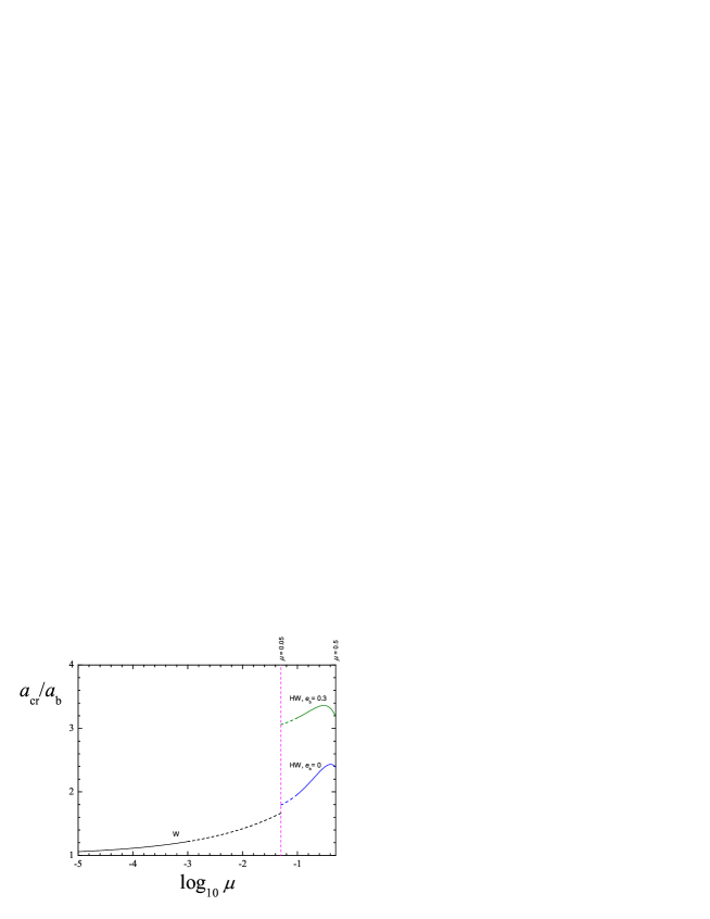
Figure 2: “Mass parameter–critical semimajor axis” analytical relationships. Curve “W”: Wisdom’s law, given by Equation (3). Curves “HW”: Holman–Wiegert’s empirical relation, given by Equation (4), at two values of the central binary eccentricity. Extrapolations are dashed. The vertical dashed (magenta) line shows the theoretical threshold $\mu=0.05$.

Let us look at the “junction” of the two relations in more detail. In Figure 2, the “mass parameter–critical semimajor axis” analytical relationships are presented graphically. Wisdom’s law is valid, as derived, at $e_{\mathrm{b}}=0$; Holman–Wiegert’s curve, constructed for $e_{\mathrm{b}}=0$, joins Wisdom’s curve, as one can see, rather smoothly, though a moderate jump may be present in the “uncertainty interval” around the $\mu$ threshold value.

As pointed out in Quillen & Faber (2006), at $\mu\leq 0.001$ and $e_{\mathrm{b}}<0.3$ the chaotic zone size is independent of $e_{\mathrm{b}}$ and is described by Wisdom’s law. Therefore, it is adequate to compare how Wisdom’s and Holman–Wiegert’s relations join, if $e_{\mathrm{b}}=0.3$. From Figure 2, it is evident that a jump or a sharp rise should be definitely present in the “uncertainty interval”, i.e., the chaotic zone size increases sharply somewhere in the interval. In other words, in the eccentric case, the transition from one mechanism of chaos generation (overlap of $(p+1)$:$p$ resonances) to another one (overlap of $p$:1 resonances) seems to result not only in the change of the diffusion character, but also in the sharp increase of the chaotic zone size.

Independent evidence for the $\mu$ threshold value follows from the fact that the derived $\mu$ threshold roughly corresponds to the $\mu$ value at which the loss of stability of the triangular Lagrangian points L₄ and L₅ takes place (this value is $\approx 0.04$, see Szebehely 1967). Though this might seem to be merely a coincidence, physically it looks quite natural that the transition to global chaos (due to overlap of $p$:1 resonances) leaves no place for regular islands in the phase space around the triangular libration points.

Besides, the threshold existence seems to explain an old numerical-experimental result by Nacozy (1976) that the Sun–Jupiter–Saturn system becomes unstable on increasing $\mu$ 29 times, i.e., up to $\sim 0.03$—rather close to $0.05$, taking into account that the problem differs from the restricted one. Recently, Kholshevnikov & Kuznetsov (2011) obtained an even smaller numerical-experimental value of $\mu$ for the system gross instability upsurge, namely, $\mu\sim 0.02$. Again, since the problem setting is somewhat different, one may say that the numerical-experimental value roughly agrees with our theoretical prediction. The differences between the theoretical and numerical-experimental values can be due to the extrapolative character of the former as well.

Further on, in Section 6, we compare the theoretical prediction for the threshold directly with relevant observational data on exoplanetary systems.

5 Stability diagrams and the criterion predictions

Let us consider an example of our theory application concerning circumbinary exoplanets. Nowadays, several circumbinary planets in systems of main-sequence binaries are known; Kepler-16b is the prototype, discovered in 2011 by Doyle et al. (2011). In Popova & Shevchenko (2013), stability diagrams in the “pericentric distance–eccentricity” plane were constructed, which show that Kepler-16b is in a hazardous vicinity to the global instability domain: the planet resides just between the instability “teeth” in the space of orbital parameters. Kepler-16b is safe inside a resonance cell bounded by the unstable 5/1 and 6/1 resonances. The planets Kepler-34b and Kepler-35b, reported in Welsh et al. (2012), are also safe inside resonance cells at the chaos border (Popova & Shevchenko, 2013).

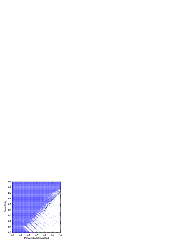
Figure 3: Stability diagram for Kepler-16b. The chaotic domain is shown by the shaded area, as revealed numerically in Popova & Shevchenko (2013). The critical curve, given by Equation (14) at $\mu=0.227$, is superimposed (extrapolation is dashed). The green dot indicates the actual location of planet Kepler-16b. The red triangle indicates the instability border location, as given by the Holman–Wiegert criterion at zero eccentricity.

In Figure 3, the curve $e_{\mathrm{cr}}(q)$, given by Equation (14), is superimposed on the stability diagram constructed in Popova & Shevchenko (2013) for Kepler-16b by means of numerically integrating the equations of planetary motion and computing the Lyapunov spectra. The motion is regarded as chaotic, if the maximum Lyapunov exponent is non-zero. The location of planet Kepler-16b is shown in Figure 3 by a green dot. The instability border location, as given by the Holman–Wiegert criterion (Equation (4)), is shown by a red triangle; note that its location coincides with the extrapolation of the curve $e_{\mathrm{cr}}(q)$ to zero eccentricity. (Such an agreement is in fact rather fortuitous because the Holman–Wiegert value has been calculated here for the actual value of the binary eccentricity $e_{\mathrm{b}}=0.159$, whereas the analytical expression for $e_{\mathrm{cr}}(q)$ was derived setting $e_{\mathrm{b}}=0$.)

One can see that the $e_{\mathrm{cr}}(q)$ curve approximately describes the smoothed border of the chaotic zone in Figure 3. In fact, the real border is ragged; the most prominent “teeth” correspond to the integer $p$:1 resonances. The Farey tree (Meiss, 1992) of resonant “teeth” at the border is evident. (Consider the lowest order “neighboring” resonances $m/n$ and $m^{\prime}/n^{\prime}$; in the given case, these are the integer mean motion resonances $m/1$ and $(m+1)/1$. The lower level of the Farey tree is made of “mediants” given by the formula $m^{\prime\prime}/n^{\prime\prime}=(m+m^{\prime})/(n+n^{\prime})=(2m+1)/2$. Thus, the half-integer mean motion resonances are the mediants for the integer ones, and so on.) The resonances densely accumulate higher in the diagram, on approaching the parabolic separatrix. The diagram graphically demonstrates how the resonances (beginning with the 4/1, 5/1, 6/1 resonances on the left of the figure) overlap. Note that the 5/1 nd 6/1 resonant “teeth” engulf the cell where the planet is located.

6 The mass parameter threshold and the diversity of observed exosystems

In this section, we discuss the relevance of the mass parameter threshold to the diversity of the observed orbital configurations of exosystems. How well does the theoretical prediction for the $\mu$ threshold agree with the observational data? To explore this, let us construct an empirical relationship between the primaries’ mass parameter $\mu$ and the ratio of the tertiary and secondary orbital periods $T_{\mathrm{out}}/T_{\mathrm{in}}$, based on a relevant sample of exosystems. For this purpose, we use the exoplanetary data provided by the Exoplanet Encyclopedia (www.exoplanet.eu), as on 2014 June 30.

Two classes of exosystems are directly relevant: biplanetary (a star plus two planets) and circumbinary (two stars plus one planet orbiting them both). Besides, for our criterion to be applicable, it is required that the planet in the outermost orbit have the smallest mass in the system. Solely, such systems have been included in the sample.

The resulting plot is shown in Figure 4. The dots show the location of the exosystems. The biplanetary systems all turn out to be on the left of two vertical (dotted and dashed) lines, whereas the circumbinary systems are on the right of them. The vertical dashed (magenta) line indicates the theoretical threshold $\mu=0.05$ for the appearance of the central chaotic zone. The dotted (cyan) line is drawn at $\mu=0.02$, roughly corresponding to the numerical-experimental results by Nacozy (1976) and Kholshevnikov & Kuznetsov (2011) on modeling the upsurge of instability of the Sun–Jupiter–Saturn system on raising the system mass parameter.

In Figure 4, the total absence of exosystems with $T_{\mathrm{out}}/T_{\mathrm{in}}<5$ at $\mu>0.05$ is evident, in agreement with our theoretical prediction that, at $\mu>0.05$, the central chaotic zone is formed, where the particle orbits with any initial eccentricities are subject to the unlimited chaotic diffusion, up to ejection from the system.

Two comments are in order. (1) A certain gap in the $\mu$ values exists between the two classes of exosystems comprising the sample. Indeed, in the biplanetary case the mass ratio of a central star–planet binary of the “Solar–Jovian” type is $\sim 0.001$, whereas in the circumbinary case the mass ratio of the typical main-sequence binary is $\sim 1$. We believe that the gap will be filled in the future, when more exosystems that include brown dwarfs are observed, such as systems with the primaries composed by a main-sequence star plus a brown dwarf, or systems with primaries composed by a brown dwarf plus a Jovian-type planet. A prototype of the former class system is HD202206 ($\mu\approx 0.014$), in which the inner “planet” with a mass of $\approx 17.4$ Jovian masses is most likely a brown dwarf (Correia et al., 2005); in Figure 4, the dot corresponding to this system is closest to the dotted (cyan) line. (2) As follows from Figure 4, many exosystems with $\mu<0.01$ cluster at the 2/1 orbital resonance; whereas the exosystems with $\mu>0.1$ do not seem to cluster at any integer resonance, but rather at half-integer ones. The latter fact is in accord with finding by Popova & Shevchenko (2013) that the observed circumbinary planets survive (though located close to the global instability border in the space of orbital elements) because they are safe inside resonance cells formed by unstable high-order integer resonances.

7 Conclusions

Our main conclusions are as follows.

1. The presence of the continuous chaotic zone around the gravitating binary of comparable masses is explained as being due to the overlap of resonances $p$:1 between the tertiary and the central binary, overlapping already at moderate values of $p\sim 4$–5 and accumulating at $p\to\infty$ near the parabolic separatrix.

2. At the tertiaries’ moderate eccentricities, the size of the continuous chaotic zone is about thrice the size of the binary, and it increases with the tertiary eccentricity.

3. The binary’s mass ratio, above which such a zone is present, is estimated to be $\sim 0.05$. This threshold has a notable physical meaning: above it, the tertiary, even starting from a small eccentricity, can diffuse, following the sequence of the overlapping $p$:1 resonances, up to ejection from the system; close encounters with other bodies are not required for escape.

4. The diversity of the observed orbital configurations of biplanetary and circumbinary exosystems is in accord with the existence of the primaries’ mass parameter threshold at $\mu\sim 0.02$–$0.05$.

Acknowledgments

The author is grateful to the referee for useful remarks. The author wish to thank T.V. Demidova, A.V. Melnikov, V.V. Orlov and E.A. Popova for helpful discussions and comments. This work was supported in part by the Russian Foundation for Basic Research (projects Nos. 12-02-00185 and 14-02-00464) and by the Programmes of Fundamental Research of the Russian Academy of Sciences “Fundamental Problems in Nonlinear Dynamics” and “Fundamental Problems of the Solar System Studies and Exploration”.

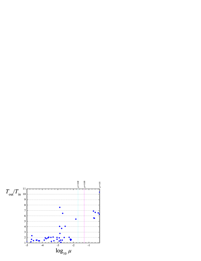
Figure 4: “Mass parameter–orbital period ratio” relationship for the biplanetary and circumbinary exosystems (dots). The vertical dashed (magenta) line shows the theoretical threshold $\mu=0.05$. The dotted (cyan) line corresponds to $\mu=0.02$, see the text.

References

- Artymowicz & Lubow (1994) Artymowicz, P., & Lubow, S. H. 1994, ApJ, 421, 651
- Artymowicz & Lubow (1996) Artymowicz, P., & Lubow, S. H. 1996, in Disks and Outflows around Young Stars, ed. S. V. W. Beckwith, J. Staude, A. M. Quetz, & A. Natta (New York: Springer), 115
- Chirikov (1959) Chirikov, B. V. 1959, Atomnaya Energiya, 6, 630 (1960, J. Nucl. Energy Part C: Plasma Phys., 1, 253)
- Chirikov (1979) Chirikov, B. V. 1979, PhR, 52, 263
- Chirikov & Vecheslavov (1986) Chirikov, B. V., & Vecheslavov, V. V. 1986, INP Preprint 86–184 (Novosibirsk: Institute of Nuclear Physics), http://www.quantware.ups-tlse.fr/chirikov/ publbinp.html
- Chirikov & Vecheslavov (2000) Chirikov, B. V., & Vecheslavov, V. V. 2000, J. Exp. Theor. Phys., 90, 562 (Zh. Eksp. Teor. Fiz., 117, 644)
- Correia et al. (2005) Correia, A. C. M., Udry, S., Mayor, M., et al. 2005, A&A, 440, 751
- Doyle et al. (2011) Doyle, L. R., Carter, J. A., Fabrycky, D. C., et al. 2011, Science, 333, 1602
- Duncan et al. (1989) Duncan, M., Quinn, T., & Tremaine, S. 1989, Icarus, 82, 402
- Holman & Wiegert (1999) Holman, M. J., & Wiegert, P. A. 1999, AJ, 117, 621
- Kholshevnikov & Kuznetsov (2011) Kholshevnikov, K. V., & Kuznetsov, E. D. 2011, Celest. Mech. Dyn. Astron., 109, 201
- Lichtenberg & Lieberman (1992) Lichtenberg, A. J., & Lieberman, M. A. 1992, Regular and Chaotic Dynamics (New York: Springer)
- Liu & Sun (1994) Liu, J., & Sun, Y. S. 1994, Celest. Mech. Dyn. Astron., 60, 3
- Mardling (2008) Mardling, R. A. 2008, in The Cambridge N-Body Lectures (Lecture Notes in Physics, Vol. 760; Berlin: Springer), 59
- Meiss (1992) Meiss, J. D. 1992, Rev. Mod. Phys., 64, 795
- Meschiari (2012) Meschiari, S. 2012, ApJ, 752, 71
- Mikkola (2008) Mikkola, S. 2008, in Multiple Stars Across the H-R Diagram, ed. S. Hubrig, M. Petr-Gotzens, & A. Tokovinin (ESA Astrophysics Symposia; Berlin: Springer), 11
- Moriwaki & Nakagawa (2004) Moriwaki, K., & Nakagawa, Y. 2004, ApJ, 609, 1065
- Mudryk & Wu (2006) Mudryk, L. R., & Wu, Y. 2006, ApJ, 639, 423
- Murray & Dermott (1999) Murray, C. D., & Dermott, S. F. 1999, Solar System Dynamics (Cambridge: Cambridge Univ. Press)
- Nacozy (1976) Nacozy, P. E. 1976, AJ, 81, 787
- Paardekooper et al. (2012) Paardekooper, S.-J., Leinhardt, Z. M., Thébault, T., et al. 2012, ApJL, 754, L16
- Petrosky (1986) Petrosky, T. Y. 1986, Phys. Lett. A, 117, 328
- Petrosky & Broucke (1988) Petrosky, T. Y., & Broucke, R. 1988, Celest. Mech. Dyn. Astron., 42, 53
- Pierens & Nelson (2007) Pierens, A., & Nelson, R. P. 2007, A&A, 472, 993
- Pierens & Nelson (2008) Pierens, A., & Nelson, R. P. 2008, A&A, 483, 633
- Popova & Shevchenko (2012) Popova, E. A., & Shevchenko, I. I. 2012, Astron. Lett., 38, 581 (Pis’ma Astron. Zhurnal, 38, 652)
- Popova & Shevchenko (2013) Popova, E. A., & Shevchenko, I. I. 2013, ApJ, 769, 152
- Quillen & Faber (2006) Quillen, A. C., & Faber, P. 2006, MNRAS, 373, 1245
- Roy & Haddow (2003) Roy, A., & Haddow, M. 2003, Celest. Mech. Dyn. Astron., 87, 411
- Saito et al. (2012) Saito, M. M., Tanikawa, K., & Orlov, V. V. 2012, Celest. Mech. Dyn. Astron., 112, 235
- Saito et al. (2013) Saito, M. M., Tanikawa, K., & Orlov, V. V. 2013, Celest. Mech. Dyn. Astron., 116, 1
- Shevchenko (2007) Shevchenko, I. I. 2007, in IAU Symp. 236, Near Earth Objects, Our Celestial Neighbors: Opportunity and Risk, ed. A. Milani, G. B. Valsecchi, & D. Vokrouhlický (Cambridge: Cambridge Univ. Press), 15
- Shevchenko (2008) Shevchenko, I. I. 2008, MNRAS, 384, 1211; 2010, MNRAS, 407, 704
- Shevchenko (2010) Shevchenko, I. I. 2010, Phys. Rev. E, 81, 066216
- Shevchenko (2011) Shevchenko, I. I. 2011, New Astronomy, 16, 94
- Shevchenko (2014) Shevchenko, I. I. 2014, Phys. Lett. A, 378, 34
- Szebehely (1967) Szebehely, V. 1967, Theory of Orbits (New York: Academic Press)
- Szebehely (1980) Szebehely, V. 1980, Celest. Mech., 22, 7
- Szebehely & McKenzie (1981) Szebehely, V., & McKenzie, R. 1981, Celest. Mech., 23, 3
- Valtonen et al. (2008) Valtonen, M., Mylläri, A., Orlov, V., et al. 2008, in IAU Symp. 246, Dynamical Evolution of Dense Stellar Systems, ed. E. Vesperini, M. Giersz, & A. Sills (Cambridge: Cambridge Univ. Press), 209
- Welsh et al. (2012) Welsh, W. F., Orosz, J. A., Carter, J. A., et al. 2012, Nature, 481, 475
- Welsh et al. (2014) Welsh, W. F., Orosz, J. A., Carter, J. A., et al. 2014, in IAU Symp. 293, Formation, Detection, and Characterization of Extrasolar Habitable Planets, ed. N. Haghighipour (Cambridge: Cambridge Univ. Press), 125
- Wisdom (1980) Wisdom, J. 1980, AJ, 85, 1122