Auger spectra following inner-shell ionization of Argon by a Free-Electron Laser

Abstract

We explore the possibility of retrieving Auger spectra with FEL radiation. Using a laser pulse of 260 eV photon energy, we study the interplay of photo-ionization and Auger processes following the initial formation of a 2p inner-shell hole in Ar. Accounting for the fine structure of the ion states we demonstrate how to retrieve the Auger spectrum of $\mathrm{Ar^{+}\rightarrow Ar^{2+}}$. Moreover, considering two electrons in coincidence we also demonstrate how to retrieve the Auger spectrum of $\mathrm{Ar^{2+}\rightarrow Ar^{3+}}$.

I Introduction

The response of atoms to intense extreme ultraviolet (XUV) and X-ray Free-Electron-Lasers (FEL) is a fundamental theory problem. In addition, understanding FEL-driven processes is of interest for accurate modeling of laboratory and astrophysical plasmas. The fast progress in generating intense FEL pulses of femtosecond duration renders timely the study of FEL driven processes in atoms. Such processes include the formation of inner-shell vacancies by photo-absorption and the subsequent Auger decays. Exploring the interplay of photo-ionization and Auger processes is a key to understanding the rich electron dynamics underlying the formation of highly charged ions Sorokin et al. (2007); Young et al. (2010); Doumy et al. (2011) and hollow atoms Young et al. (2010); Fukuzawa et al. (2013); Frasinski et al. (2013).

Auger spectra have attracted a lot of interest over the years with early studies involving the formation of an inner-shell hole following the impact of a particle, such as an electron Mehlhorn (1985); McGuire (1975a, b); Mehlhorn and Stalherm (1968); Werme et al. (1973). From the early 80s, synchrotron radiation has largely replaced particle impact as a triggering mechanism of Auger processes Von Busch et al. (1994); Alkemper et al. (1997); von Busch et al. (1999); Lablanquie et al. (2011). Such studies include the detailed Auger spectrum following the decay of Ar${}^{+}(2p^{-1})$ Pulkkinen et al. (1996); Lablanquie et al. (2007). The reason for using synchrotron radiation is that it is monochromatic and allows for well defined initial excitations in the soft and hard X-ray regime. A recent study with synchrotron radiation Huttula et al. (2013) involves the measurement of Auger spectra following the decay of the $\mathrm{Ar}^{2+}(2p^{-1}v^{-1})$ ionic states; $v^{-1}$ is a hole in a valence orbital and $\mathrm{Ar}^{2+}(2p^{-1}v^{-1})$ is formed by single-photon double ionization.

In this work, we explore the feasibility of obtaining detailed Auger spectra using FEL radiation. FEL radiation allows for well-defined initial excitations. It also allows for the creation of multiple inner-shell holes resulting in multiple Auger decays; generally the Auger spectra thus generated have larger yields than those generated from synchrotron radiation. The increasing availability of FEL sources provides an additional motivation for the current study. We explore the interplay of photo-ionization and Auger processes in $\mathrm{Ar}$ interacting with a 260 eV FEL pulse, a photon energy sufficient to ionize a single inner-shell $\mathrm{2p}$ electron in Ar. We compute the ion yields due to Auger and photo-ionization processes and study the ion yields dependence on the FEL pulse parameters. To do so we solve a set of rate equations Rohringer and Santra (2007); Makris et al. (2009). Initially, in the rate equations we only account for the electronic configuration of the ion states. This simplification allows us to gain insight into the processes involved and explore the optimal parameters for observing Auger spectra. We next proceed to fully account for the fine structure of the ion states in the rate equations. We subsequently obtain the detailed Auger spectrum of $\mathrm{Ar^{+}\rightarrow Ar^{2+}}$. Moreover, we demonstrate how the detailed Auger spectrum of $\mathrm{Ar^{2+}\rightarrow Ar^{3+}}$ can be observed in an FEL two-electron coincidence experiment.

II Auger and Ion yields excluding fine structure

We model the response of Ar to a 260 eV FEL pulse by formulating and solving a set of rate equations for the time dependent populations of the ion states Rohringer and Santra (2007); Makris et al. (2009). Our first goal is to gain insight into how the ion and Auger yields depend on the duration and intensity of the laser pulse. To do so, in this section, we simplify the theoretical treatment by accounting only for the electronic configuration, i.e, $(1s^{a},2s^{b},2p^{c},3s^{d},3p^{e})$ of the ion states and not the fine structure of these states. By fine structure we refer to all possible ${}^{2S+1}L_{J}$ states for a given electronic configuration, accounting for spin-orbit coupling. To compute the Auger transition rates between different electron configurations we use the formalism introduced by Bhalla et al. Bhalla et al. (1973) and refer to these transition rates as Auger group rates in accord with Bhalla et al. (1973).

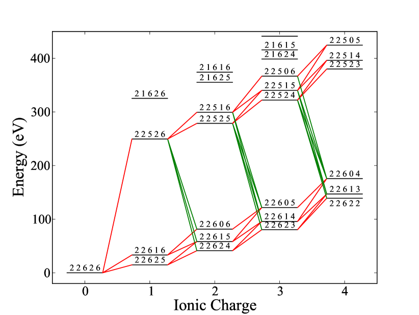
Figure 1: (Color online) Ionization pathways between different electronic configurations of Ar, up to Ar⁴⁺, accessible with sequential single-photon ($\mathrm{\hbar\omega=260eV})$ absorptions and Auger decays. The label $\mathrm{(a,b,c,d,e)}$ stands for the electronic configuration $\mathrm{(1s^{a},2s^{b},2p^{c},3s^{d},3p^{e})}$. The red and green lines indicate photo-ionization and Auger transitions, respectively.

II.1 Rate equations

In the rate equations we account for single-photon ionization and Auger transitions. For the ion states considered the X-ray fluorescence widths are typically three orders of magnitude smaller than the Auger decay widths Chen and Crasemann (1974); we can thus safely neglect the former. In Fig. 1, accounting for states up to Ar⁴⁺, we illustrate the photo-ionization and Auger transitions between states with different electron configurations that are allowed for a laser pulse of 260 eV photon energy. This photon energy is sufficient for creating a single inner-shell $\mathrm{2p}$ hole and multiple valence holes in Ar. In the rate equations we include all possible ion states accessible by a 260 eV laser-pulse; the highest ion state is $\mathrm{Ar^{9+}(1s^{2},2s^{2},2p^{5},3s^{0},3p^{0})}$. The rate equations describing the population $\mathcal{I}_{i}^{(q)}$ of an ion state $\mathrm{i}$ with charge $\mathrm{q}$ take the form

$$\frac{d}{dt} \mathcal{I}_{j}^{(q)}(t)=\sum_{i}\left(\sigma_{i\rightarrow j}J(t)+\Gamma_{i\rightarrow j}\right)\mathcal{I}_{i}^{(q-1)}(t)$$ (1)

$$-\sum_{k}\left(\sigma_{j\rightarrow k}J(t)+\Gamma_{j\rightarrow k}\right)\mathcal{I}_{j}^{(q)}(t)$$

$$\frac{d}{dt} \mathcal{A}^{(q)}_{i\rightarrow j}=\Gamma_{i\rightarrow j}\mathcal{I}_{i}^{(q-1)}(t),$$

$$\frac{d}{dt} \mathcal{P}^{(q)}_{i\rightarrow j}=\sigma_{i\rightarrow j}J(t)\mathcal{I}_{i}^{(q-1)}(t),$$

where $\mathrm{\sigma_{i\rightarrow j}}$ and $\mathrm{\Gamma_{i\rightarrow j}}$ are the single-photon absorption cross section and Auger decay rate from initial state $\mathrm{i}$ to final state $\mathrm{j}$, respectively. $\mathrm{J(t)}$ is the photon flux. Atomic units are used in this work. The temporal form of the FEL flux is modelled with a Gaussian function Rohringer and Santra (2007) which is given by

$$J(t)=1.554\times 10^{-16}\frac{I_{0}\textrm{[W cm}^{-2}]}{\hbar\omega\textrm{[eV]}}\exp\left\{-4\ln 2\left(\frac{t}{\tau_{X}}\right)^{2}\right\}$$ (2)

with $\mathrm{\tau_{X}}$ the full width at half maximum and $\mathrm{I_{0}}$ the peak intensity. The first term in Eq. (1) accounts for the formation of the state $\mathrm{j}$ with charge $\mathrm{q}$ through the single-photon ionization and Auger decay of the state $\mathrm{i}$ with charge $\mathrm{q-1}$. The second term in Eq. (1) accounts for the depletion of state $\mathrm{j}$ by single-photon ionization and Auger decay to the state $\mathrm{k}$ with charge $\mathrm{q+1}$. In Eq. (1), we also solve for the Auger yield $\mathcal{A}^{(q)}_{i\rightarrow j}$ from an initial state $\mathrm{i}$ with charge $\mathrm{q-1}$ to a final state $\mathrm{j}$ with charge $\mathrm{q}$. In addition, we solve for the photo-ionization yield $\mathcal{P}^{(q)}_{i\rightarrow j}$ from an initial state $\mathrm{i}$ with charge $\mathrm{q-1}$ to a final state $\mathrm{j}$ with charge $\mathrm{q}$. These yields provide the probability for observing an electron with energy corresponding to the transition $\mathrm{i\rightarrow j}$. The total Auger and photo-ionization yields for the transition from any state with charge $\mathrm{q-1}$ to any state with charge $\mathrm{q}$ are given by

$$\mathcal{A}^{(q)}=\sum_{i,j}\mathcal{A}^{(q)}_{i\rightarrow j}, \mathcal{P}^{(q)}=\sum_{i,j}\mathcal{P}^{(q)}_{i\rightarrow j}.$$ (3)

To find the total ion yield of a state with charge $\mathrm{q}$, i.e., the ion yield for Ar^q+ we sum over the populations of all ion states with charge $\mathrm{q}$

$$\mathcal{I}^{(q)}=\sum_{i}\mathcal{I}_{i}^{(q)}.$$ (4)

All yields are computed long after the end of the pulse.

As we show later in the paper, it is also of interest to compute the Auger and photo-ionization yields along a pathway $\mathrm{i\rightarrow j\rightarrow k}$. These yields provide the probability for observing in a two-electron coincidence experiment two electrons with energies corresponding to the transitions $\mathrm{i\rightarrow j}$ and $\mathrm{j\rightarrow k}$. If there is only one state $\mathrm{i}$ leading to state $\mathrm{j}$ then the probability for observing the electron emitted in the transition $\mathrm{i\rightarrow j}$ and the electron emitted in the transition $\mathrm{j\rightarrow k}$ is simply the Auger $\mathcal{A}^{(q)}_{j\rightarrow k}$ or the photo-ionization $\mathcal{P}^{(q)}_{j\rightarrow k}$ yield. However, it can be the case that we have multiple states leading to state $\mathrm{j}$, for example, $\mathrm{i\rightarrow j\rightarrow k}$ and $\mathrm{i^{\prime}\rightarrow j\rightarrow k}$. Then to compute the probability $\mathcal{P}^{(q)}_{j(i)\rightarrow k}$ or $\mathcal{A}^{(q)}_{j(i)\rightarrow k}$ for observing the electron emitted in the transition $\mathrm{i\rightarrow j}$ and the electron emitted in the transition $\mathrm{j\rightarrow k}$ we need to solve separately for the contribution of state $\mathrm{i}$ to the population of state $\mathrm{j}$:

$$\frac{d}{dt}\mathcal{I}^{(q-1)}_{j(i)}(t)= (\sigma_{i\rightarrow j}J(t)+\Gamma_{i\rightarrow j})\mathcal{I}^{(q-2)}_{i}(t)$$ (5)

$$-\sum_{k^{\prime}}(\sigma_{j\rightarrow k^{\prime}}J(t)+\Gamma_{j\rightarrow k^{\prime}})\mathcal{I}^{(q-1)}_{j(i)}(t)$$

$$\frac{d}{dt}\mathcal{P}^{(q)}_{j(i)\rightarrow k}= \sigma_{j\rightarrow k}J(t)\mathcal{I}^{(q-1)}_{j(i)}(t)$$

$$\frac{d}{dt}\mathcal{A}^{(q)}_{j(i)\rightarrow k}= \Gamma_{j\rightarrow k}\mathcal{I}^{(q-1)}_{j(i)}(t).$$

II.2 Auger group rates

To compute the Auger group rates $\Gamma_{i\rightarrow j}$ we use the formulation of Bhalla et al. Bhalla et al. (1973). For each electron configuration included in the rate equations, we obtain the energy and bound atomic orbital with a Hartree-Fock (HF) calculation. These calculations are performed with the ab initio quantum chemistry package molpro Werner et al. (2009) using the split-valence 6-311G basis set. To compute the continuum orbital that describes the outgoing Auger electron we use the Hartree-Fock-Slater (HFS) one-electron potential that is obtained using an updated version of the Herman Skillman atomic structure code Herman and Skillman (1963); Pauli . This one electron potential is expressed in terms of an effective nuclear charge $\mathrm{Z_{\text{HFS}}(r)}$. The resulting radial HFS equation is of the form

$$\left[-\frac{d^{2}}{dr^{2}}+\frac{l(l+1)}{r^{2}}-\frac{Z_{\text{HFS}}(r)}{r}\right]P_{nl}(r)=EP_{nl}(r),$$ (6)

where the orbital wavefunction is given by $\mathrm{\psi_{nlm}(\mathbf{r})=r^{-1}P_{nl}(r)Y_{lm}(\hat{r})}$. We solve equation Eq. (6) for the continuum orbital ($\mathrm{E>0}$) using the modified Numerov method Numerov (1933); Melkanoff et al. (1966). We match the solution to the appropriate asymptotic boundary conditions for energy normalized continuum wave functions Child (1974). In Table I we list our results for the Auger group rates $\mathrm{Ar^{+}(2p^{-1})\rightarrow Ar^{2+}(3s^{-1}3p^{-1})}$, $\mathrm{Ar^{+}(2p^{-1})\rightarrow Ar^{2+}(3s^{-2})}$ and $\mathrm{Ar^{+}(2p^{-1})\rightarrow}$ $\mathrm{Ar^{2+}(3p^{-2})}$ and compare them with two other calculations that employ the HFS method McGuire (1971) and the HF method Dyall and Larkins (1982) both for the bound and the continuum orbitals. As expected, our results lie between the results of these two calculations. For reference, we also list in Table I the results from a Configurational Interaction (CI) calculation Dyall and Larkins (1982). In Table II we list our results for all the Auger group rates involved in the rate equations for Ar for a 260 eV FEL pulse.

Table 1: Auger group rates for a transition from an initial state $\mathrm{(1s^{a},2s^{b},2p^{c},3s^{c},3p^{e})}$ to a final state where the electron filling in the $\mathrm{2p}$ hole in the initial state and the electron escaping to the continuum occupy $\mathrm{nl}$ and $\mathrm{n^{\prime}l^{\prime}}$ orbitals. We also list the Auger rates obtained in McGuire (1971) using the Hartree-Fock-Slater (HFS) method, in Dyall and Larkins (1982) using a Hartree-Fock (HF) method, and in Dyall and Larkins (1982) using a CI calculation. The rates are given in 10^-4 a.u.

initial config.					method	group rates ($10^{-4}$ a.u.)
a	b	c	d	e		$3s3s$	$3s3p$	$3p3p$	total
2	2	5	2	6	HFS McGuire (1971)	0.77	12.85	47.90	61.52
					HF Dyall and Larkins (1982)	0.28	15.74	56.97	72.99
					CI Dyall and Larkins (1982)	0.47	9.54	54.74	64.75
					this work	0.45	15.60	51.67	67.72

Table 2: As in Table I for results obtained in this work for all Auger group rates included in the rate equations.

initial config.					group rates ($10^{-4}$ a.u.)
a	b	c	d	e	$3s3s$	$3s3p$	$3p3p$	total
2	2	5	2	6	0.450	15.598	51.665	67.713
2	2	5	2	5	0.502	9.615	25.457	35.575
2	2	5	1	6	-	9.244	58.693	67.937
2	2	5	2	4	0.568	9.429	20.324	30.321
2	2	5	1	5	-	5.780	29.273	35.053
2	2	5	0	6	-	-	68.708	68.708
2	2	5	2	3	0.638	7.973	11.680	20.291
2	2	5	1	4	-	5.631	23.952	29.583
2	2	5	0	5	-	-	33.761	33.761
2	2	5	2	2	0.710	5.845	4.349	10.905
2	2	5	1	3	-	4.650	13.337	17.986
2	2	5	0	4	-	-	23.946	23.946
2	2	5	2	1	0.778	2.843	-	3.621
2	2	5	1	2	-	3.374	4.909	8.283
2	2	5	0	3	-	-	14.309	14.309
2	2	5	2	0	0.863	-	-	0.863
2	2	5	1	1	-	1.612	-	1.612
2	2	5	0	2	-	-	5.168	5.168

II.3 Results for Auger and Ion yields

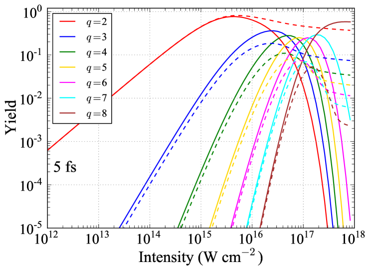
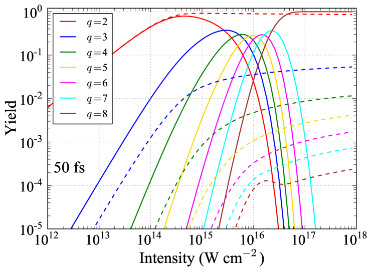
Figure 2: (Color online) Total ion $\mathcal{I}^{(q)}$ (solid lines) and Auger $\mathcal{A}^{(q)}$ (dashed lines) yields as a function of intensity for pulse duration of 5 fs (top) and 50 fs (bottom).

For the photo-ionization cross sections we use the Los Alamos National Laboratory atomic physics codes LAN that are based on the HF routines of R. D. Cowan Cowan (1981). Assuming that the initial state is the neutral Ar, we solved numerically Press (2007) the set of first order differential rate equations in Eq. (1). In Fig. 2 we show our results for the total ion $\mathcal{I}^{(q)}$ and Auger $\mathcal{A}^{(q)}$ yields as a function of the pulse intensity for pulse durations of 5 fs and 50 fs. From Fig. 2 we observe that $\mathcal{A}^{(q)}$ can be very similar to $\mathcal{I}^{(q)}$ for $q\geq 2$ depending on the pulse intensity and duration. Indeed, the formation of $\mathrm{Ar^{q+}}$ occurs from a sequence of transitions where the final step involves either the single-photon ionization or the Auger decay of $\mathrm{Ar^{(q-1)+}}$. For high pulse intensities, independent of the pulse duration, both final steps are likely and thus $\mathcal{A}^{(q)}$ is different than $\mathcal{I}^{(q)}$. For small pulse intensities, if the pulse is short then the formation of $\mathrm{Ar^{q+}}$ through the Auger decay of $\mathrm{Ar^{(q-1)+}}$ is favored; if the pulse is long multi-photon absorption is highly likely making possible formation of $\mathrm{Ar^{q+}}$ also through single-photon ionization of $\mathrm{Ar^{(q-1)+}}$. Thus, generally, for small pulse intensities, if the pulse is short $\mathcal{A}^{(q)}\approx\mathcal{I}^{(q)}$ while if the pulse is long $\mathcal{A}^{(q)}\neq\mathcal{I}^{(q)}$.

II.4 Truncation of the number of states included in the rate equations

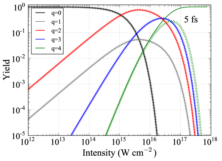
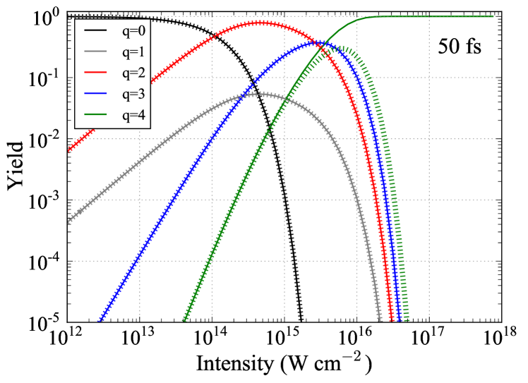
Figure 3: (Color online) Total ion yields $\mathcal{I}^{(q)}$ for $q=$ 0,1,2,3,4 when ion states up to Ar⁹⁺ (dashed lines) and ion states up to Ar⁴⁺ (solid lines) are included as a function of pulse intensity for pulse durations 5 fs (top) and 50 fs (bottom).

Fig. 2 shows that appropriate tuning of the laser parameters can result in large Auger yields even for high ion states. Regarding Auger spectra this is an advantage of FEL radiation compared to synchrotron radiation. However, discerning the Auger spectra produced by the FEL pulse is a challenging task since many photo-ionization and Auger electrons escape to the continuum. In the next section we focus on the Auger electron spectra resulting from ion states up to Ar³⁺. To accurately describe these spectra we need to account for the fine structure of the ion states included in the rate equations. However, such an inclusion results in a very large increase of the number of ion states that need to be accounted for in the rate equations. For instance, when considering states up to Ar⁴⁺ the number of ions states in the rate equations increases from 21(no fine structure) to 186 (with fine structure). We thus truncate the number of ion states we consider. In Fig. 3 we compare $\mathcal{I}^{(q)}$, for $\mathrm{q=}$ 1,2,3,4, when we include ion states up to Ar⁹⁺ and up to Ar⁴⁺. We find that the truncation affects only $\mathcal{I}^{(4)}$ while $\mathcal{I}^{(1)}$, $\mathcal{I}^{(2)}$ and $\mathcal{I}^{(3)}$ are unaffected. Since the focus of the current work is the Auger electron spectra up to Ar³⁺, in what follows we truncate to include only ion states up to Ar⁴⁺. Moreover, comparing Fig. 3 with Fig. 2, we find that a pulse duration of 5 fs is short enough for $\mathcal{A}^{(q)}\approx\mathcal{I}^{(q)}$ to be true for intensities up to roughly $10^{16}$ W cm^-2. This guarantees that less photo-ionization electrons are ejected to the continuum making it easier to discern the Auger electrons. We also find that for pulse intensities around $10^{15}$-$10^{16}$ W cm^-2 both $\mathcal{A}^{(2)}$ and $\mathcal{A}^{(3)}$ yields have significant values. Thus, a laser pulse with duration of 5 fs and intensity of $5\times 10^{15}$ W cm^-2 is optimal for the experimental observation of the Auger electron spectra up to Ar³⁺.

III Auger spectra

III.1 Computation of fine structure ion states

We next describe the method we use to compute the fine structure states of each electron configuration that is included in the truncated rate equations. To obtain the fine structure ion states we use the grasp2k package Jönsson et al. (2013) and the relci extension Fritzsche et al. (2002) provided in the ratip package Fritzsche (2012). These packages are used to perform relativistic calculations within the Multi-Configuration Dirac-Hartree-Fock (MCDHF) formalism Grant (2006). The photo-ionization cross sections and Auger decay rates between fine structure states are then calculated using the photo and auger components of the ratip package. Since grasp2k utilizes the Dirac equation the calculations are performed in the $j$-$j$ coupling scheme. We briefly outline the steps we follow to obtain the fine structure states for a given electron configuration of Ar; where appropriate we illustrate using Ar${}^{+}(1s^{2},2s^{2},2p^{5},3s^{2},3p^{6})$.

1) We identify the fine structure states for the electron configuration at hand; in our example these states are $\mathrm{{}^{2}P_{1/2}}$ and $\mathrm{{}^{2}P_{3/2}}$. We identify the configurational state functions (CSFs) that can be constructed out of the possible $\mathrm{nlj}$ orbitals; in our example the possible CSFs are

$$1.(1s_{1/2}^{2},2s_{1/2}^{2},2p_{1/2}^{1},2p_{3/2}^{4},3s_{1/2}^{2},3p_{1/2}^{2},3p_{3/2}^{4});J^{P}=\frac{1}{2}^{-}$$

$$2.(1s_{1/2}^{2},2s_{1/2}^{2},2p_{1/2}^{2},2p_{3/2}^{3},3s_{1/2}^{2},3p_{1/2}^{2},3p_{3/2}^{4});J^{P}=\frac{3}{2}^{-}$$

Each fine structure state is a linear combination of the CSFs that have the same total angular momentum $J$ and parity $P$; in our example $\mathrm{{}^{2}P_{1/2}}$ is expressed in terms of the first CSF and $\mathrm{{}^{2}P_{3/2}}$ in terms of the second CSF. A Self-Consistent-Field (SCF) DHF calculation is now performed for all the CSFs. This calculation optimizes the $\mathrm{nlj}$ orbitals and the coefficients in the expansion of each fine structure state in terms of CSFs.

2) To account for electron correlation, as a first step, we include the additional orbitals $\mathrm{3d_{3/2}}$ and $\mathrm{3d_{5/2}}$. A new set of CSFs is generated from the single and double excitations of the step-1 CSFs, while keeping the occupation of the $\mathrm{1s}$, $\mathrm{2s}$ and $\mathrm{2p}$ orbitals frozen. A new MCDHF calculation is then performed with the new set of CSFs keeping the step-1 $\mathrm{nlj}$ orbitals frozen and only optimizing the newly added ones.

3) As a second step in accounting for electron correlation, we include all orbitals up to $\mathrm{4d_{3/2}}$, $\mathrm{4d_{5/2}}$. Again, as for step-2, a new set of CSFs is generated from the single and double excitations of the step-1 CSFs, while keeping the occupation of the $1s$, $2s$ and $2p$ orbitals frozen. Another MCDHF calculation is performed optimizing only the newly added, compared to step-2, orbitals. Introducing correlation orbitals layer by layer as described in steps 1-3 is the recommended procedure in the grasp2k manual in order to achieve convergence of the SCF calculations.

4) Finally, using the orbitals generated in steps 1-3 we perform a CI calculation that optimizes the coefficients that express each fine structure state in terms of all the CSFs generated in steps 1-3.

Table 3: The Auger energies and rates from the $\mathrm{Ar(2p^{-1}_{1/2}})$ and $\mathrm{Ar(2p^{-1}_{3/2}})$ initial state to a final state where the electron filling in the $\mathrm{2p}$ hole and the electron escaping to the continuum occupy $\mathrm{nl}$ and $\mathrm{n^{\prime}l^{\prime}}$ orbitals. We list the MCDHF results obtained in this work and the experimental results of Pulkkinen et al. Pulkkinen et al. (1996). The Auger electron energies $\mathrm{E}$ are given in eV and the Auger rates $\Gamma$ are given in $10^{-4}$ a.u.

Final State		Exp. Pulkkinen et al. (1996)		this work
		$E$	$I$	$E$	$\Gamma$	$I$
Ar${}^{+}(2p_{1/2}^{-1}$)
$3p3p$	${}^{3}P_{2}$	207.39	76	207.57	2.37	64
	${}^{3}P_{1}$	207.25	176	207.44	5.11	138
	${}^{3}P_{0}$	207.20	60	207.38	2.13	58
	${}^{1}D_{2}$	205.65	404	205.64	11.78	318
	${}^{1}S_{0}$	203.26	100	203.35	3.70	100
$3s3p$	${}^{3}P_{2}$	-	-	193.25	0.02	1
	${}^{3}P_{1}$	193.13	24	193.12	1.12	30
	${}^{3}P_{0}$	193.07	18	193.06	0.58	16
	${}^{1}P_{1}$	189.50	39	188.66	1.85	50
$3s3s$	${}^{1}S_{0}$	176.43	6	175.36	0.62	17
Ar${}^{+}(2p_{3/2}^{-1}$)
$3p3p$	${}^{3}P_{2}$	205.24	261	205.43	7.58	240
	${}^{3}P_{1}$	205.10	73	205.30	2.77	88
	${}^{3}P_{0}$	205.08	26	205.24	0.73	23
	${}^{1}D_{2}$	203.50	390	203.50	11.01	348
	${}^{1}S_{0}$	201.11	100	201.22	3.16	100
$3s3p$	${}^{3}P_{2}$	191.09	77	191.11	1.52	48
	${}^{3}P_{1}$	190.95	11	190.98	0.35	11
	${}^{3}P_{0}$	-	-	190.92	0	0
	${}^{1}P_{1}$	187.39	71	186.52	1.79	57
$3s3s$	${}^{1}S_{0}$	174.27	13	173.22	0.61	19

In Table  3 we list the energies and Auger rates we obtain using the method described above for the fine structure states of Ar${}^{+}(2p^{-1})$. To directly compare with the experimental results in Pulkkinen et al. (1996) we define the intensity for an Auger decay from an initial state $\mathrm{i}$ to a final state $\mathrm{j}$ as

$$I_{i\rightarrow j}=\frac{\Gamma_{i\rightarrow j}}{\sum_{j}\Gamma_{i\rightarrow j}},$$ (7)

and is scaled such that the intensity for the transition $\mathrm{Ar^{+}(2p^{-1})\rightarrow Ar^{2+}(3p^{-2};^{1}S_{0})}$ is equal to 100 in accord with Pulkkinen et al. (1996). It can be seen that our calculated results are in good agreement with the experimental results of Pulkkinen et al. Pulkkinen et al. (1996).

III.2 Results for Auger and Ion yields including fine structure

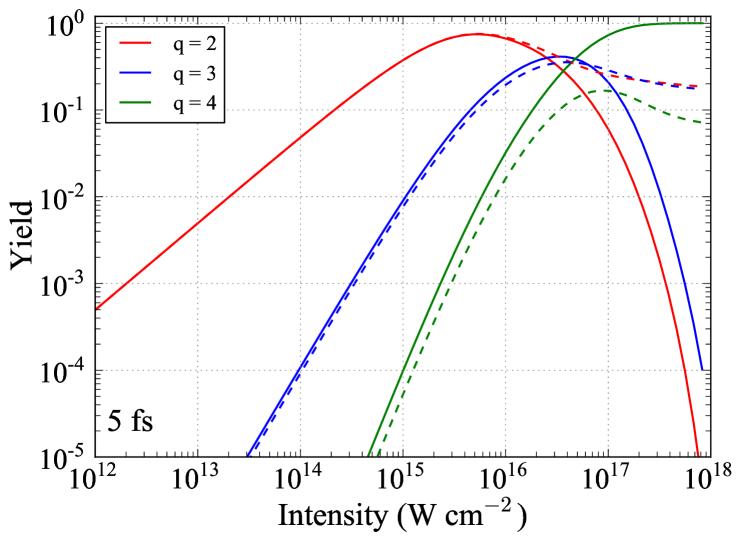
Figure 4: (Color online) Total ion $\mathcal{I}^{(q)}$ (solid lines) and Auger $\mathcal{A}^{(q)}$ yields (dashed lines) for $q=2,3,4$ as a function of intensity for a pulse duration of 5 fs. These yields are calculated with fine structure included in the rate equations.

In Fig. 4 we show the total ion $\mathcal{I}^{(q)}$ and Auger $\mathcal{A}^{(q)}$ yields accounting for fine structure for a pulse duration of 5 fs. We find that these yields are very similar to the yields obtained in the previous section where fine structure was neglected. Thus our conclusions in the previous section regarding optimal laser parameters for observing the Auger electron spectra up to $\mathrm{Ar^{3+}}$ still hold. Also in Fig. 5 we plot the Auger yields $\mathcal{A}_{i\rightarrow j}^{(2)}$ and $\mathcal{A}_{\i\rightarrow j}^{(3)}$ for all possible $\mathrm{i}$, $\mathrm{j}$ fine structure states.

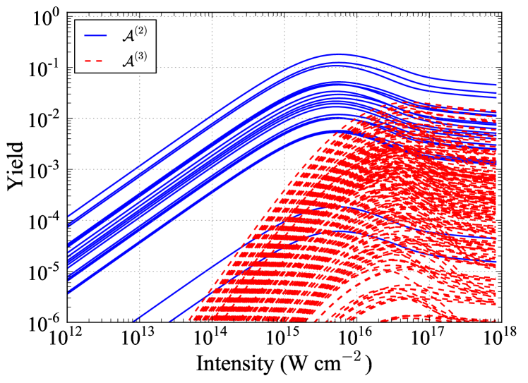
Figure 5: (Color online) The Auger yields $\mathcal{A}^{(2)}_{i\rightarrow j}$ (blue, solid lines) and $\mathcal{A}^{(3)}_{i\rightarrow j}$ (red, dashed lines) as a function of intensity for a pulse duration of 5 fs. These yields are calculated with fine structure included in the rate equations.

III.3 Auger spectra including fine structure

III.3.1 One-electron Auger spectra

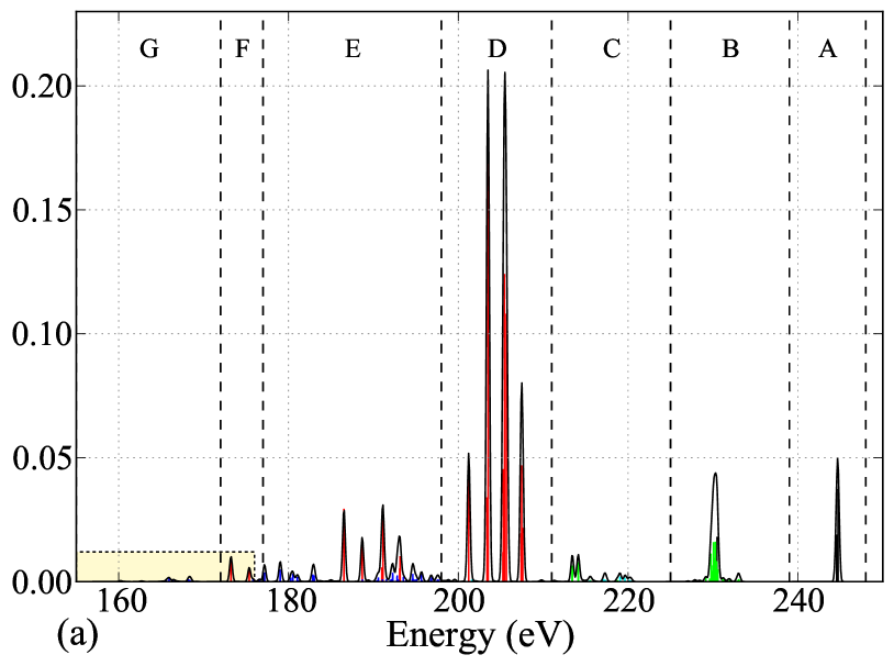
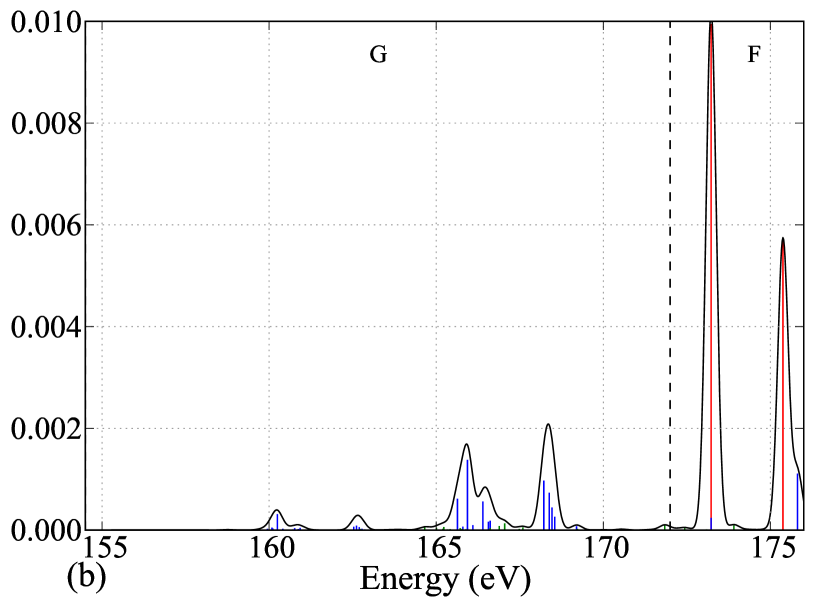
Figure 6: (Color online) The electron spectra for a 5 fs, 260 eV pulse with an intensity of $5\times 10^{15}$ W cm^-2 for energies between 150 and 250 eV (a) and energies between 155 and 177 eV (b). For clarity the plot range of (b) is highlighted in yellow in (a). The peaks are convoluted by 0.37 eV FWHM Gaussian functions. The peaks of the photo-ionization electrons emitted during transitions from the initial states Ar (black) and Ar⁺ (green) are in the energy ranges denoted by A, B, and C (see Table IV). The peaks of the Auger electrons emitted during the transitions $\mathrm{Ar^{+}(2p^{-1})\rightarrow Ar^{2+}}$ (red) are in the energy ranges denoted by D, E, and F, and the ones emitted during the transitions $\mathrm{Ar^{2+}(2p^{-1}v^{-1})\rightarrow Ar^{3+}}$ (blue) are in the energy ranges denoted by E, F, and G (see Table IV).

In Fig. 6 we compute the electron spectra for a 260 eV FEL pulse with $5\times 10^{15}$ W cm^-2 intensity and 5 fs duration. Both the Auger $\mathcal{A}^{(q)}_{i\rightarrow j}$ and photo-ionization $\mathcal{P}_{i\rightarrow j}^{(q)}$ yields for charges up to $q=4$ contribute to the peaks in these electron spectra. To account for the energy uncertainty of a 5 fs pulse, which is 0.37 eV, we have convoluted the peaks in Fig. 6 with Gaussian functions of 0.37 eV FWHM. We find that the energies of the photo-ionization electrons ejected in the transition $\mathrm{Ar}^{+}\rightarrow\mathrm{Ar}^{2+}$ (peak height $\mathcal{P}_{i\rightarrow j}^{(2)}$) are well separated from the energies of the Auger electrons ejected in the transitions $\mathrm{Ar}^{+}\rightarrow\mathrm{Ar}^{2+}$ (peak height $\mathcal{A}^{(2)}_{i\rightarrow j}$) and $\mathrm{Ar}^{2+}\rightarrow\mathrm{Ar}^{3+}$ (peak height $\mathcal{A}^{(3)}_{i\rightarrow j}$); the photo-ionization peaks are above 210 eV while the Auger peaks are below 210 eV. In Fig. 6 and Table 4, the energy range of the photo-ionization electrons is denoted by A, B, C; the energy range of the Auger electrons emitted during transitions from the initial states Ar⁺ and Ar²⁺ are denoted by D, E, F, and E, F, and G, respectively. In Fig. 6 we see that the Auger yields $\mathcal{A}^{(2)}_{i\rightarrow j}$ (D, E, F) are much larger than all other Auger yields in the same energy range. They can thus be discerned and measured for the laser parameters under consideration. The Auger yields $\mathcal{A}^{(3)}_{i\rightarrow j}$ (E, F, G) are smaller but still visible, while the Auger yields $\mathcal{A}^{(4)}_{i\rightarrow j}$ are too small to be discerned in Fig. 6. However, except for the energy region below 170 eV, the Auger electron spectra resulting from the transitions $\mathrm{Ar}^{2+}\rightarrow\mathrm{Ar}^{3+}$ overlap with the Auger electron spectra resulting from the transitions $\mathrm{Ar}^{+}\rightarrow\mathrm{Ar}^{2+}$. Thus, in order to discern and be able to experimentally observe the latter Auger electron spectra we need to consider spectra of two electrons in coincidence. We do so in what follows.

Table 4: Labeling of energy regions in the electron spectrum shown in Fig. 6. $e^{-}_{\rm p}$ and $e^{-}_{\rm A}$ stand for photo-ionization and Auger electrons, respectively. $u^{-1}$ represents a hole in any of the $2p$, $3s$ or $3p$ orbitals.

Region	Transitions
$A$	Ar$+\hbar\omega\rightarrow$Ar${}^{+}(3p^{-1})+e^{-}_{\rm P}$
$B$	Ar$+\hbar\omega\rightarrow$Ar${}^{+}(3s^{-1})+e^{-}_{\rm P}$
$B$	Ar${}^{+}(u^{-1})+\hbar\omega\rightarrow$Ar${}^{2+}(u^{-1}3p^{-1})+e^{-}_{\rm P}$
$C$	Ar${}^{+}(u^{-1})+\hbar\omega\rightarrow$Ar${}^{2+}(u^{-1}3s^{-1})+e^{-}_{\rm P}$
$D$	Ar${}^{+}(2p^{-1})\rightarrow$Ar${}^{2+}(3p^{-2})+e^{-}_{\rm A}$
$E$	Ar${}^{+}(2p^{-1})\rightarrow$Ar${}^{2+}(3s^{-1}3p^{-1})+e^{-}_{\rm A}$
$F$	Ar${}^{+}(2p^{-1})\rightarrow$Ar${}^{2+}(3s^{-2})+e^{-}_{A}$
$E,F,G$	Ar${}^{2+}(2p^{-1}v^{-1})\rightarrow$Ar${}^{3+}(v^{-3})+e^{-}_{A}$

III.3.2 Two-electron coincidence Auger spectra

We now consider the electron spectra resulting from the transitions:

$$\mathrm{Ar}+\hbar\omega\rightarrow\mathrm{Ar}^{+}(2p^{-1})+e^{-}_{P}\rightarrow\mathrm{Ar}^{3+}+e^{-}_{P}+e^{-}_{B}+e^{-}_{C}$$ (8)

The photo-ionization electron $\mathrm{e_{P}^{-}}$ has an energy of 12.3 eV for $\mathrm{Ar}^{+}(2p^{-1}_{3/2})$ and 10.2 eV for $\mathrm{Ar}^{+}(2p^{-1}_{1/2})$. This energy is very different from the energies of electrons $\mathrm{e_{B}^{-}}$ and $\mathrm{e_{C}^{-}}$. It thus suffices to plot in coincidence the energies of electrons $\mathrm{e_{B}^{-}}$ and $\mathrm{e_{C}^{-}}$. We note that many coincidence experiments have been performed with synchrotron radiation Alkemper et al. (1997); Lablanquie et al. (2007, 2011); Huttula et al. (2013). While some coincidence experiments have been performed with FEL radiation Kurka et al. (2009); Rudenko et al. (2010) the low repetition rate poses a challenge. Advances in FEL sources should overcome such challenges in the near future.

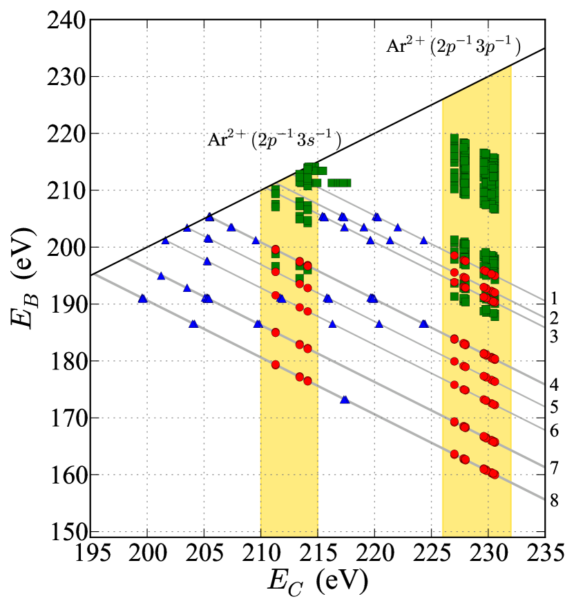
Figure 7: (Color online) Two-electron coincidence spectra for Ar${}^{+}(2p_{3/2}^{-1})\rightarrow$Ar${}^{3+}(v^{-3})$ generated by a 5 fs, $5\times 10^{15}$ W cm^-2 FEL pulse. We show the spectrum below the $E_{B}=E_{C}$ line for the PPP (green squares), PAP (blue triangles) and PPA (red circles) transition sequences, see text for details. The Ar${}^{3+}(3p^{-3})$ final fine structure states are labeled as 1:${}^{4}S$, 2:${}^{2}D$, 3:${}^{2}P$, the Ar${}^{3+}(3s^{-1}3p^{-2})$ states as 4:${}^{4}P$, 5:${}^{2}D$, 6:${}^{2}S$, 7:${}^{2}P$, and the Ar${}^{3+}(3s^{-2}3p^{-1})$ state as 8:${}^{2}P$. The energy range of the PPA transition sequences $\mathrm{Ar^{+}(2p^{-1})\rightarrow Ar^{2+}(2p^{-1}3s^{-1})\rightarrow Ar^{3+}}$ and $\mathrm{Ar^{+}(2p^{-1})\rightarrow Ar^{2+}(2p^{-1}3p^{-1})\rightarrow Ar^{3+}}$ are highlighted by yellow.

In Fig. 7 we plot in coincidence the energies of electrons $\mathrm{e^{-}_{B}}$ and $\mathrm{e^{-}_{C}}$. Specifically, Fig. 7 corresponds to the $\mathrm{Ar^{+}(2p^{-1}_{3/2})}$ fine structure state in Eq. (8). We only show the spectrum that lies below the line $E_{B}=E_{C}$ (black solid line), with $E_{B}$ the energy of electron $\mathrm{e_{B}^{-}}$ and $E_{C}$ the energy of electron $\mathrm{e_{C}^{-}}$. Since the two electrons are indistinguishable, the remaining spectrum can be obtained by a reflection with respect to the line $E_{B}=E_{C}$ of the spectrum shown in Fig. 7. From Eq. (8) it follows that each line with $E_{B}+E_{C}=constant$, grey lines in Fig. 7, scans the spectra of electrons emitted from transitions in Eq. (8) through any possible fine structure state of Ar²⁺ to the same fine structure state of Ar³⁺. The spectra of the electrons emitted from the transitions in Eq. (8) can be labelled according to the sequence of photo-ionization (P) and Auger processes (A) involved while transitioning from Ar to Ar³⁺: PPA (red in Fig. 7), PPP (green) and PAP (blue). Our goal is to retrieve the Auger electron spectra corresponding to the transitions $\mathrm{Ar^{2+}\rightarrow Ar^{3+}}$. These latter spectra are the ones labelled as PPA in Fig. 7; we highlight the energy range of the $\mathrm{e_{B}^{-}}$ and $\mathrm{e_{C}^{-}}$ electrons emitted in the PPA transition sequences $\mathrm{Ar^{+}(2p^{-1})\rightarrow Ar^{2+}(2p^{-1}3s^{-1})\rightarrow Ar^{3+}}$ and $\mathrm{Ar^{+}(2p^{-1})\rightarrow Ar^{2+}(2p^{-1}3p^{-1})\rightarrow Ar^{3+}}$. Thus to be able to retrieve the Auger electron spectra associated with the transitions $\mathrm{Ar^{2+}\rightarrow Ar^{3+}}$ we must be able to discern the PPA from the PPP and the PAP transition sequences. We see that in the highlighted area in Fig. 7 there is some small overlap of the PPA with the PPP and PAP sequences. However, we find that the height of the peaks of the PPA transition sequences are much larger than the height of the peaks of the PPP and PAP transition sequences. Specifically, the total Auger yield $\mathcal{A}^{(3)}$ associated with the PPA transition sequences is roughly 5 times larger than the photo-ionization yield $\mathcal{P}^{(3)}_{PAP}$ corresponding to the PAP transition sequences and 10 times larger than the photo-ionization yield $\mathcal{P}^{(3)}_{PPP}$ corresponding to the PPP transition sequences, with $\mathcal{P}^{(3)}_{PAP}+\mathcal{P}^{(3)}_{PPP}=\mathcal{P}^{(3)}$. To show that this is indeed the case we show in Fig. 8 the contour plot of the two-electron coincidence spectra associated with the highlighted area in Fig. 7 corresponding to the transitions $\mathrm{Ar^{+}(2p^{-1})\rightarrow Ar^{2+}(2p^{-1}3s^{-1})\rightarrow Ar^{3+}}$. Note that the height of the peaks in Fig. 8 is given by $\mathcal{A}^{(3)}_{j\rightarrow k}$ or $\mathcal{A}^{(3)}_{j(i)\rightarrow k}$ (see discussion in section IIA) for the PPA transition sequences while the height is $\mathcal{P}^{(3)}_{j\rightarrow k}$ or $\mathcal{P}^{(3)}_{j(i)\rightarrow k}$ for the PPP and PAP transition sequences. Each coincidence peak has been convoluted by a 0.37 eV FWHM Gaussian function. We find that all except one of the observable peaks in Fig. 8 are due to PPA transition sequences; the small height peak at $(E_{C}=211.7,E_{B}=190)$ is due to a PAP sequence. We have thus demonstrated that we can retrieve from the two-electron coincidence spectra the Auger electron spectra associated with the transitions $\mathrm{Ar^{2+}\rightarrow Ar^{3+}}$. We note that a similar discussion and conclusions hold for the Auger spectra corresponding to the $\mathrm{Ar^{+}(2p^{-1}_{1/2})}$ fine structure state in Eq. (8).

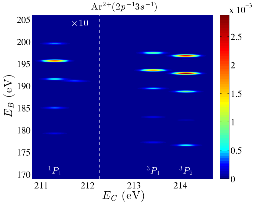
Figure 8: (Color online) Two-electron coincidence spectra for $\mathrm{Ar^{+}(2p^{-1})\rightarrow Ar^{2+}(2p^{-1}3s^{-1})\rightarrow Ar^{3+}}$ for the $\mathrm{Ar^{2+}(2p^{-1}3s^{-1})}$ fine structure states $\mathrm{{}^{1}P_{1}}$, $\mathrm{{}^{3}P_{1}}$ and $\mathrm{{}^{3}P_{2}}$. The peaks of the spectra corresponding to the Ar${}^{2+}(2p^{-1}3s^{-1};^{1}P_{1})$ fine structure state, to the left of the vertical dashed-white line, are much smaller than the rest of the spectra and we have thus multiplied them by a factor of 10 so that they are visible. The coincidence peaks have been convoluted by 0.37 eV FWHM Gaussian functions.

Finally we note that our calculations neglect satellite structure. That is, we do not account for Auger transitions where one electron fills in the 2p hole, another one escapes to the continuum while a third one is promoted to an excited state. The main (larger) satellite Auger yields we are neglecting are most likely due to the Ar${}^{+}(2p^{-1})\rightarrow$Ar${}^{2+}(3s^{-1}3p^{-1})$ transitionPulkkinen et al. (1996). However, these satellite yields are smaller than the main Auger yields for this transition. In addition, these satellite Auger yields would only contribute to the part of the spectrum corresponding to PAP transition sequences in the energy region $E_{B}=$170 -180 eV and $E_{C}=$210-220 eV. But as we discussed above the contribution to the electron spectra from PAP transition sequences is smaller than the contribution from the PPA transition sequences. Thus our approximation is justified.

IV Conclusions

We have explored the interplay of photo-ionization and Auger transitions in Ar when interacting with a 260 eV FEL pulse. Solving the rate equations we have explored the dependence of the ion and Auger yields on the laser parameters accounting, at first, only for the electron configuration of the ion states. We have found that an FEL pulse of roughly 5 fs duration and $5\times 10^{15}$ Wcm^-2 intensity is optimal for retrieving Auger electron spectra up to Ar³⁺. Secondly, we have account for the fine structure of the ionic states and have truncated the rate equations to include states only up to $\mathrm{Ar^{4+}}$. We have shown how the Auger electron spectra of $\mathrm{Ar^{+}\rightarrow Ar^{2+}}$ can be retrieved. We have also shown that the Auger electron spectra of $\mathrm{Ar^{2+}\rightarrow Ar^{3+}}$ can also be retrieved when two electrons are considered in coincidence. We have thus demonstrated that interaction with FEL radiation is a possible route for retrieving Auger electron spectra. We believe that our work will stimulate further theoretical and experimental studies along these lines.

V Acknowledgments

The authors are grateful to Prof. P. Lambropoulos for initial motivation and valuable discussions. A.E. acknowledges support from EPSRC under Grant No. H0031771 and J0171831 and use of the Legion computational resources at UCL.

References

- Sorokin et al. (2007) A. A. Sorokin, S. V. Bobashev, T. Feigl, K. Tiedtke, H. Wabnitz, and M. Richter, Phys. Rev. Lett. 99, 213002 (2007).
- Young et al. (2010) L. Young, E. P. Kanter, B. Krässig, Y. Li, A. M. March, S. T. Pratt, R. Santra, S. H. Southworth, N. Rohringer, L. F. DiMauro, et al., Nature 466, 56 (2010).
- Doumy et al. (2011) G. Doumy, C. Roedig, S. K. Son, C. Blaga, A. D. DiChiara, R. Santra, N. Berrah, C. Bostedt, J. D. Bozek, P. H. Bucksbaum, et al., Phys. Rev. Lett. 106, 83002 (2011).
- Fukuzawa et al. (2013) H. Fukuzawa, S.-K. Son, K. Motomura, S. Mondal, K. Nagaya, S. Wada, X.-J. Liu, R. Feifel, T. Tachibana, Y. Ito, et al., Phys. Rev. Lett. 110, 173005 (2013).
- Frasinski et al. (2013) L. J. Frasinski, V. Zhaunerchyk, M. Mucke, R. J. Squibb, M. Siano, J. H. D. Eland, P. Linusson, P. v. d. Meulen, P. Salén, R. D. Thomas, et al., Phys. Rev. Lett. 111, 073002 (2013).
- Mehlhorn (1985) W. Mehlhorn, Atomic Inner-Shell Physics (Plenum, New York, 1985).
- McGuire (1975a) E. J. McGuire, Phys. Rev. A 11, 10 (1975a).
- McGuire (1975b) E. J. McGuire, Phys. Rev. A 11, 1880 (1975b).
- Mehlhorn and Stalherm (1968) W. Mehlhorn and D. Stalherm, Z. Phys. 217, 294 (1968).
- Werme et al. (1973) L. O. Werme, T. Bergmark, and K. Siegbahn, Phys. Scr. 8, 149 (1973).
- Von Busch et al. (1994) F. Von Busch, J. Doppelfeld, C. Gunther, and E. Hartmann, J. Phys. B: At. Mol. Opt. Phys. 27, 2151 (1994).
- Alkemper et al. (1997) U. Alkemper, J. Doppelfeld, and F. Von Busch, Phys. Rev. A 56, 2741 (1997).
- von Busch et al. (1999) F. von Busch, U. Kuetgens, J. Doppelfeld, and S. Fritzsche, Phys. Rev. A 59, 2030 (1999).
- Lablanquie et al. (2011) P. Lablanquie, S. M. Huttula, M. Huttula, L. Andric, J. Palaudoux, J. H. D. Eland, Y. Hikosaka, E. Shigemasa, K. Ito, and F. Penent, Phys. Chem. Chem. Phys. 13, 18355 (2011).
- Pulkkinen et al. (1996) H. Pulkkinen, S. Aksela, O. P. Sairanen, A. Hiltunen, and H. Aksela, J. Phys. B: At. Mol. Opt. Phys. 29, 3033 (1996).
- Lablanquie et al. (2007) P. Lablanquie, L. Andric, J. Palaudoux, U. Becker, M. Braune, J. Viefhaus, J. H. D. Eland, and F. Penent, J. Elec. Spec. Rel. Phenom. 156, 51 (2007).
- Huttula et al. (2013) S. M. Huttula, P. Lablanquie, L. Andric, J. Palaudoux, M. Huttula, S. Sheinerman, E. Shigemasa, Y. Hikosaka, K. Ito, and F. Penent, Phys. Rev. Lett. 110, 113002 (2013).
- Rohringer and Santra (2007) N. Rohringer and R. Santra, Phys. Rev. A 76, 033416 (2007).
- Makris et al. (2009) M. G. Makris, P. Lambropoulos, and A. Mihelič, Phys. Rev. Lett. 102, 033002 (2009).
- Bhalla et al. (1973) C. P. Bhalla, N. O. Folland, and M. A. Hein, Phys. Rev. A 8, 649 (1973).
- Chen and Crasemann (1974) M. H. Chen and B. Crasemann, Phys. Rev. A 10, 2232 (1974).
- Werner et al. (2009) H.-J. Werner, P. J. Knowles, G. Knizia, F. R. Manby, M. Schütz, et al., “Molpro, version 2009.1, a package of ab initio programs,” (2009), see http://www.molpro.net.
- Herman and Skillman (1963) F. Herman and S. Skillman, Atomic structure calculations (Prentice-Hall, New Jersey, 1963).
- (24) M. D. Pauli, http://hermes.phys.uwm.edu/projects/elecstruct/hermsk/HS.TOC.html.
- Numerov (1933) B. Numerov, Publs. Observatoire Central Astrophys. Russ. 2, 188 (1933).
- Melkanoff et al. (1966) M. A. Melkanoff, T. Sawada, and J. Raynal, Methods Comp. Phys. 6, 1 (1966).
- Child (1974) M. S. Child, Molecular Collision Theory (Academic Press, London, 1974).
- McGuire (1971) E. J. McGuire, Phys. Rev. A 3, 1801 (1971).
- Dyall and Larkins (1982) K. G. Dyall and F. P. Larkins, J. Phys. B: At. Mol. Phys. 15, 2793 (1982).
- (30) “Los Alamos National Laboratory Atomic Physics Codes,” see http://aphysics2.lanl.gov/tempweb/lanl/.
- Cowan (1981) R. D. Cowan, The theory of atomic structure and spectra (University of California Press, 1981).
- Press (2007) W. H. Press, Numerical Recipes: The art of scientific computing, 3rd ed. (Cambridge University Press, 2007).
- Jönsson et al. (2013) P. Jönsson, G. Gaigalas, J. Bieroń, C. Froese Fischer, and I. P. Grant, Comput. Phys. Commun. 184, 2197 (2013).
- Fritzsche et al. (2002) S. Fritzsche, C. Froese Fischer, and G. Gaigalas, Comput. Phys. Commun. 148, 103 (2002).
- Fritzsche (2012) S. Fritzsche, Comput. Phys. Commun. 183, 1525 (2012).
- Grant (2006) I. P. Grant, Relativistic Quantum Theory of Atoms and Molecules: Theory and Computation (Springer Series on Atomic, Optical, and Plasma Physics) (Springer-Verlag New York, Inc., 2006).
- Kurka et al. (2009) M. Kurka, A. Rudenko, L. Foucar, K. U. Kühnel, Y. H. Jiang, T. Ergler, T. Havermeier, M. Smolarski, S. Schössler, K. Cole, et al., J. Phys. B: At. Mol. Opt. Phys. 42, 141002 (2009).
- Rudenko et al. (2010) A. Rudenko, Y. H. Jiang, M. Kurka, K. U. Kühnel, L. Foucar, O. Herrwerth, M. Lezius, M. F. Kling, C. D. Schröter, R. Moshammer, et al., J. Phys. B: At. Mol. Opt. Phys. 43, 194004 (2010).