Algebraic moment closure for population dynamics on discrete structures

Abstract

Moment closure on general discrete structures often requires one of the following: (i) an absence of short closed loops (zero clustering); (ii) existence of a spatial scale; (iii) ad hoc assumptions. Algebraic methods are presented to avoid the use of such assumptions for populations based on clumps, and are applied to both SIR and macroparasite disease dynamics. One approach involves a series of approximations that can be derived systematically, and another is exact and based on Lie algebraic methods.

1 Introduction

1.1 Motivation

In modelling biological systems, we typically have (at least) three objectives: enhanced scientific understanding of the system in question; the ability to answer counterfactual questions relating to possible perturbations of the system; and a framework for working with data to estimate values of important parameters statistically. Having a low-dimensional model is of benefit for each of these aims since such simple models are typically analytically more transparent and numerically more efficient than complex high-dimensional models.

Increasingly, models of infectious disease transmission take place on a network to represent the heterogeneities that exist in contacts between hosts (Danon et al., 2011). This is a major benefit for model realism, however in the situation where $N$ distinct individuals are in one of $\Sigma$ epidemiological states then $\Sigma^{N}$ variables are needed to describe the system state. A low-dimensional description of such dynamics is therefore essential if we seek understanding, optimisation of intervention strategies or statistical inference in the large-$N$ regime.

1.2 Background

Many different approaches exist to enable dimensional reduction of high-dimensional models. Perhaps the most commonly used is Kirkwood’s superposition principle (Kirkwood and Boggs, 1942). In the context of biology, this approach has been applied to infectious diseases (Keeling, 1999), including rapid modelling of emerging disease threats (Ferguson et al., 2001). Such equations are intended to be used in the case of relatively homogeneous populations, but with significant transitivity in the pairwise interactions. Here, transitivity is used to imply the presence of a significant number of triangles in the network of interactions between individuals, which would be called ‘clustered’ in network theoretical language that we adopt here. While these moment closures are often in excellent agreement with simulation, they lack a priori justification meaning we cannot be clear about exactly when they will fail.

One class of populations where there is potentially significant transitivity in the network of interactions and where some analytical progress can be made are spatial models. Here individuals are located at points in space and the interaction strength between them decays as the distance between them increases, with $L$ being the natural length scale of the interaction. Here, the pioneering work of Ovaskainen and Cornell (2006), and Cornell and Ovaskainen (2008) demonstrated how asymptotically exact results could be obtained to avoid these concerns by perturbative expansion in an inverse spatial length scale $L^{-1}$.

For non-clustered but heterogeneous populations, work by Ball and Neal (2008) has also showed how asymptotically exact epidemic equations can be derived that are at worst of dimensionality $2N$, with more sophisticated limit theorems (Decreusefond et al., 2012) showing that the four-dimensional equations of Volz (2008) can be derived – and indeed the dimensionality of these equations can be further reduced to one (Miller, 2011; Miller et al., 2012). Such insights can be applied to non-spatial clustered populations if there is a local-global distinction, to provide sets of ODEs whose dimensionality, while often large, can be independent of $N$ (House, 2010; Volz et al., 2011; Ma et al., 2013).

At the same time, there are innovative approaches to non-exact clustered moment closure, including: projection operator methods (Dodd and Ferguson, 2007); analytic consideration of asymptotic early growth (House and Keeling, 2010); maximum entropy methods (Rogers, 2011); non-independent Bernoulli trials (Taylor et al., 2012); and a priori distributions (Kiss and Simon, 2012). These often significantly improve closure performance, but remain essentially ad hoc.

1.3 Algebraic methods

This paper considers an algebraic approach to moment closure for clustered populations based on ‘clump’ models, but generalisable to other local-global structures. This can take the form either of a series of approximations or an exact solution based on Lie algebras. As such it provides a potential new route to rigorous moment closure for clustered discrete structures. We will first introduce some general methods for time-inhomogeneous ODE systems, then will apply these to SIR epidemics and macroparasite ecology.

2 Algebraic solution of time-inhomogeneous ODEs

2.1 General theory

Suppose we have a time-inhomogeneous set of ODEs that are written in matrix / vector form as

$$\frac{\mathrm{d}\mathbf{p}}{\mathrm{d}t}=\mathbf{M}(t)\mathbf{p}\text{ .}$$ (1)

We will seek solutions to this equation of the form

$$\mathbf{p}(t)={\rm e}^{\mathbf{Z}(t)}\mathbf{p}(0)\text{ .}$$ (2)

The case where $\mathbf{M}$ does not depend on time was considered in the context of epidemic dynamics by Keeling and Ross (2008), and offers significant computational advantages. There are a variety of approaches to the solution of the more general case outlined in a particularly comprehensive paper by Wilcox (1967), the conventions from which will in general be used here. We will consider two such approaches.

2.2 The Magnus expansion

The first approach we will consider is a series expansion introduced by Magnus (1954), which has previously been used to solve equations like (1) applied to population dynamics (Ross, 2012). Here we start by re-writing (1) as

$$\frac{\mathrm{d}\mathbf{p}}{\mathrm{d}t}=\mu\mathbf{M}(t)\mathbf{p}\text{ .}$$ (3)

Substituting (2) into (3) then gives the relation

$$\mu\mathbf{M}(t)=\int_{0}^{1}\mathbf{G}(t,u)\mathrm{d}u\text{ ,}\qquad\text{for}\quad\mathbf{G}(t,u)={\rm e}^{u\mathbf{Z}(t)}\dot{\mathbf{Z}}(t){\rm e}^{-u\mathbf{Z}(t)}\text{ ,}$$ (4)

where we use a dot to denote derivatives with respect to time. Since this integral cannot be performed directly in the most general case, we consider a series

$$\mathbf{Z}(t)={\sum_{k=1}^{\infty}\mu^{k}\boldsymbol{\Omega}_{k}(t)}\text{ .}$$ (5)

We will refer to the truncation of the infinite sum at $\boldsymbol{\Omega}_{m}$ as the Order $m$ approximation. Substituting (5) into (4) and equating terms at the same order in $\mu$ (after which point we set $\mu=1$ without loss of generality) gives a sequence of matrices, with the first three being

$$\boldsymbol{\Omega}_{1}(t) =\int_{t_{1}=0}^{t}\mathbf{M}(t_{1})\mathrm{d}t_{1}\text{ ,}$$ (6)

$$\boldsymbol{\Omega}_{2}(t) =\frac{1}{2}\int_{t_{1}=0}^{t}\int_{t_{2}=0}^{t_{1}}[\mathbf{M}(t_{1}),\mathbf{M}(t_{2})]\mathrm{d}t_{1}\mathrm{d}t_{2}\text{ ,}$$

$$\boldsymbol{\Omega}_{3}(t) =\frac{1}{6}\int_{t_{1}=0}^{t}\int_{t_{2}=0}^{t_{1}}\int_{t_{3}=0}^{t_{2}}\left([[\mathbf{M}(t_{1}),\mathbf{M}(t_{2})],\mathbf{M}(t_{3})]+[[\mathbf{M}(t_{3}),\mathbf{M}(t_{2})],\mathbf{M}(t_{1})]\right)\mathrm{d}t_{1}\mathrm{d}t_{2}\mathrm{d}t_{3}\text{ .}$$

Here the matrix commutator $[\mathbf{A},\mathbf{B}]:=\mathbf{A}\mathbf{B}-\mathbf{B}\mathbf{A}$. The convergence of such an expansion is considered by Blanes et al. (1998), who argue that convergence will occur for times $t$ such that

$$\|\boldsymbol{\Omega}_{1}(t)\|<\xi\text{ ,}$$ (7)

and provide the numerical estimate $\xi\approx 1.086869$. Note that this is a sufficient but not necessary condition for convergence so matrices with larger norm can still be part of a convergent series.

2.3 Lie algebra methods

Now suppose that we can write

$$\mathbf{M}(t)=\sum_{i=1}^{l}a_{i}(t)\mathbf{H}_{i}\text{ ,}$$ (8)

where the $\{\mathbf{H}_{i}\}_{i=1}^{l}$ is a set of linearly independent matrices obeying

$$[\mathbf{H}_{i},\mathbf{H}_{j}]=\sum_{k=1}^{l}{\zeta_{ij}}^{k}\mathbf{H}_{k}\text{ ,}\qquad{\zeta_{ij}}^{k}\in\mathbb{C}\text{ .}$$ (9)

Such matrices form a representation of a Lie algebra, and we will now leave the range $1,\ldots l$ for indices $i,j,\ldots$ implicit for notational compactness. We then follow Wilcox (1967) and note that $\mathbf{G}(t,u)$ as in (4) obeys the following system of differential equations:

$$\frac{\partial\mathbf{G}}{\partial u}=[\mathbf{Z}(t),\mathbf{G}(t,u)]\text{ ;}\qquad\mathbf{G}(t,0)=\dot{\mathbf{Z}}(t)\text{ .}$$ (10)

In general, these equations are not an improvement on (4), however when the Lie algebra decomposition (8) is possible, we can expand other matrices in the same basis

$$\mathbf{Z}(t)=\sum_{i}\alpha_{i}(t)\mathbf{H}_{i}\text{ ,}\qquad\mathbf{G}(t,u)=\sum_{i}\mathcal{A}_{i}(t,u)\mathbf{H}_{i}\text{ ,}$$ (11)

and use the linear independence of the $\mathbf{H}_{i}$ to solve for $\mathbf{Z}(t)$.

3 Clump-based epidemics

3.1 Model definition

A highly influential paper by Ball et al. (1997) considered epidemics on networks with ‘two levels of mixing’ in which the population is split into $m$ fully connected ‘clumps’ (or ‘cliques’ in network theoretical terminology) of size $n$, so that $N=m\times n$. The large-population limit is taken with $m\rightarrow\infty$ at constant finite $n$; this leads to a natural interpretation of the population structure as a network with the ‘small worlds’ property of significant clustering within the clumps, but small mean shortest path lengths due to the random nature of links between clumps.

One of the most common applications of this work is to households, which are an important locus of disease transmission and also a natural unit for the collection of epidemiological data. Then $n$ is the size of a household, which will typically be several orders of magnitude smaller than the whole population size $N$. Variable household sizes can easily be included in this framework, but here we keep $n$ fixed to simplify the analysis.

While the analysis of Ball et al. (1997) mainly concerned the early and late behaviour of an epidemic in a population of clumps / households, later work modelled temporal dynamics and intervention strategies using ‘self-consistent’ equations (Ghoshal et al., 2004; Dodd and Ferguson, 2007; House and Keeling, 2008, 2009). For SIR epidemics these take the form of $(n+1)(n+2)/2$ ODEs, which hold in the large-$N$ limit,

$$\frac{\mathrm{d}}{\mathrm{d}t}{p}_{s,i} =\gamma\left(-ip_{s,i}+(i+1)p_{s,i+1}\right)$$ (12)

$$\quad+\tau\left(-sip_{s,i}+(s+1)(i-1)p_{s+1,i-1}\right)$$

$$\quad+\beta I(t)\left(-sp_{s,i}+(s+1)p_{s+1,i-1}\right)\text{ .}$$

Here $p_{s,i}(t)$ is interpreted as the proportion of clumps with $s$ susceptible and $i$ infectious individuals at time $t$, meaning that $p_{s,i}=0$ if $s+i>n$. $\gamma$ is the recovery rate, $\tau$ is the rate of within-clump transmission and $\beta$ is the rate of between-clump transmission. It will be convenient to define quantities

$${\sigma}_{s,i}:=s/n\text{ ,}\quad{\iota}_{s,i}:=i/n\text{ ,}\quad{v}_{s,i}=si/n\text{ .}$$ (13)

Like $p_{s,i}$, these have two indices and so are 2-tensors, however since the possible number of states is finite, we can easily concatenate columns to work with vectors $\mathbf{p}(t)$, $\boldsymbol{\sigma}$, $\boldsymbol{\iota}$ and $\mathbf{v}$. While $p_{s,i}$ is a proportion rather than a probability, since clumps are not created or destroyed in the model $\mathbf{p}$ has very similar properties to a probability vector and its elements sum to unity. In vector notation, we have the following expressions for the proportions of the population susceptible and infectious:

$$S(t):=\boldsymbol{\sigma}\cdot\mathbf{p}(t)\text{ ,}\qquad I(t):=\boldsymbol{\iota}\cdot\mathbf{p}(t)\text{ .}$$ (14)

The definitions (13) and (14), together with (12), define the high-dimensional system for closure. Of course, such a system already achieves independence of $N$, but accounting for local clustering can still lead to high dimensionality. Our task will be to derive a set of ODEs whose dimensionality does not depend on $n$ or $N$.

3.2 Standard moment closure

We now consider existing moment closure approaches. Both maximum entropy and the use of Ansätze would lead to the assumption that $p_{s,i}$ is a multinomial probability mass function for $n$ trials with probabilities $S$ and $I$ of observing susceptible and infective on each trial. Kirkwood’s superposition principle would simply involve the direct assumption that the probability of a pair of distinct individuals in the same clump being susceptible-infective is equal to the product $S\times I$, meaning that all standard approaches would lead to the substitution

$$\mathbf{v}\cdot\mathbf{p}\rightarrow(n-1)SI\text{ ,}$$ (15)

which can be combined with (18) to make a closed system. We call this the ‘mean-field’ model.

3.3 Order 1 algebraic moment closure

We now consider how algebraic approaches such as the Magnus expansion can be applied to the question of moment closure. We first note that two manipulations of the full self-consistent field equations (12) are possible. The first of these is to write them in the form of (1),

$$\frac{\mathrm{d}\mathbf{p}}{\mathrm{d}t}=(\mathbf{H}+I(t)\mathbf{K})\mathbf{p}\text{ .}$$ (16)

We can then apply the Order 1 Magnus expansion given in (6) to the system (16), assuming that $I(t)$ is a known function, to give

$$\boldsymbol{\Omega}_{1}(t)=\mathbf{H}t+\mathbf{K}\int_{t_{1}=0}^{t}I(t_{1})\mathrm{d}t_{1}=:\mathbf{H}t+\mathbf{K}C(t)\text{ .}$$ (17)

The second manipulation of (12) involves taking the inner product of these equations with each of $\boldsymbol{\sigma}$ and $\boldsymbol{\iota}$ to give an unclosed pair of ODEs that generalise the standard SIR model,

$$\frac{\mathrm{d}S}{\mathrm{d}t} =-\beta SI-\tau\mathbf{v}\cdot\mathbf{p}\text{ ,}$$ (18)

$$\frac{\mathrm{d}I}{\mathrm{d}t} =\beta SI-\gamma I+\tau\mathbf{v}\cdot\mathbf{p}\text{ .}$$

We can then substitute (17) into (5) to obtain a matrix exponential approximation to $\mathbf{v}\cdot\mathbf{p}$, provided the cumulative incidence of infection $C(t)$ is known. Fortunately, $C(t)$ can be seen to obey a simple ODE from its definition. This leads to a set of three ODEs approximating the full dynamics,

$$\frac{\mathrm{d}S}{\mathrm{d}t} =-\beta SI-\tau\mathbf{v}\cdot\mathrm{exp}\left(\mathbf{H}t+\mathbf{K}C(t)\right)\mathbf{p}(0)\text{ ,}$$ (19)

$$\frac{\mathrm{d}I}{\mathrm{d}t} =\beta SI-\gamma I+\tau\mathbf{v}\cdot\mathrm{exp}\left(\mathbf{H}t+\mathbf{K}C(t)\right)\mathbf{p}(0)\text{ ,}$$

$$\frac{\mathrm{d}C}{\mathrm{d}t} =I(t)\text{ .}$$

It is worth spending some time on consideration of the intuitive interpretation of this closure regime, which is equivalent to the assumption that $\mathbf{p}(t)=\mathbf{q}(u)|_{u=t}$ , where

$${\frac{\mathrm{d}{\mathbf{q}}}{\mathrm{d}u}}=\left(\mathbf{H}+\frac{C(t)}{t}\mathbf{K}\right)\mathbf{q}(u)\text{ ,}\qquad\mathbf{q}(0)=\mathbf{p}(0)\text{ .}$$ (20)

Note that $\mathbf{H}$ corresponds to the events that take place within the clump – recovery of infectives and transmission between members of the same clump – and $\mathbf{K}$ corresponds to a susceptible within the clump becoming infective due to infectives external to the clump. Therefore, we can interpret the approximation as assuming that the system state at time $t$ is equivalent to the one that would be obtained by running an epidemic with clumps each of whose susceptibles spontaneously become infective at constant rate $\beta C(t)/t$ integrated over the time period $u\in[0,t]$.

Therefore, the approximation is expected to be completely accurate if all infection external to the clumps is time-homogeneous; increased variability in $I(t)$ over the epidemic is therefore expected to lead to a less accurate approximation.

3.4 Higher order moment closure

The main attraction of the Magnus series is that it can be iterated to produce higher-order results. In particular, the Order 2 and 3 matrices are

$$\boldsymbol{\Omega}_{2}(t)=\frac{1}{2}\left(D_{1}(t)-D_{2}(t)\right)\mathbf{L}\text{ ,}\qquad\boldsymbol{\Omega}_{3}(t)=\frac{1}{6}F_{1}(t)\mathbf{Q}_{1}-F_{2}(t)\mathbf{Q}_{2}\text{ .}$$ (21)

Here we have used matrices

$$\mathbf{L}:=[\mathbf{H},\mathbf{K}]\text{ ,}\quad\mathbf{Q}_{1}:=[\mathbf{L},\mathbf{H}]\text{ ,}\quad\mathbf{Q}_{2}:=[\mathbf{L},\mathbf{K}]\text{ ,}$$ (22)

and functions satisfying ODEs

$$\frac{\mathrm{d}D_{1}}{\mathrm{d}t}=C(t)\text{ ,}\quad\frac{\mathrm{d}D_{2}}{\mathrm{d}t}=tI(t)\text{ ,}\quad\frac{\mathrm{d}E}{\mathrm{d}t}=I(t)C(t)\text{ ,}$$

$$\frac{\mathrm{d}F_{1}}{\mathrm{d}t}=2D_{2}(t)-\frac{1}{2}t^{2}I(t)-D_{1}(t)\text{ ,}\quad\frac{\mathrm{d}F_{2}}{\mathrm{d}t}=E(t)+\left(D_{2}(t)-D_{1}(t)\right)I(t)\text{ .}$$ (23)

The benefits of all approximations considered above in terms of dimensionality reduction are displayed in Table 1.

Model	Dimensionality
Full	$(n+1)(n+2)/2$
Order $1$	$3$
Order $2$	$5$
Order $3$	$8$
Mean Field	$2$

Table 1: Dimensional benefits of algebraic closure for the epidemic clump model.

3.5 Numerical results

The results of integrating the closed equations at different orders, making use of the EXPOKIT routines (Sidje, 1998), is given in Figures 1 and 2. This naïve method is used to test the accuracy of the approach and in practice it would be better to use one of several advanced numerical integration schemes designed to work efficiently with the Magnus series (Iserles and Nørsett, 1999; Blanes et al., 2002, 2013).

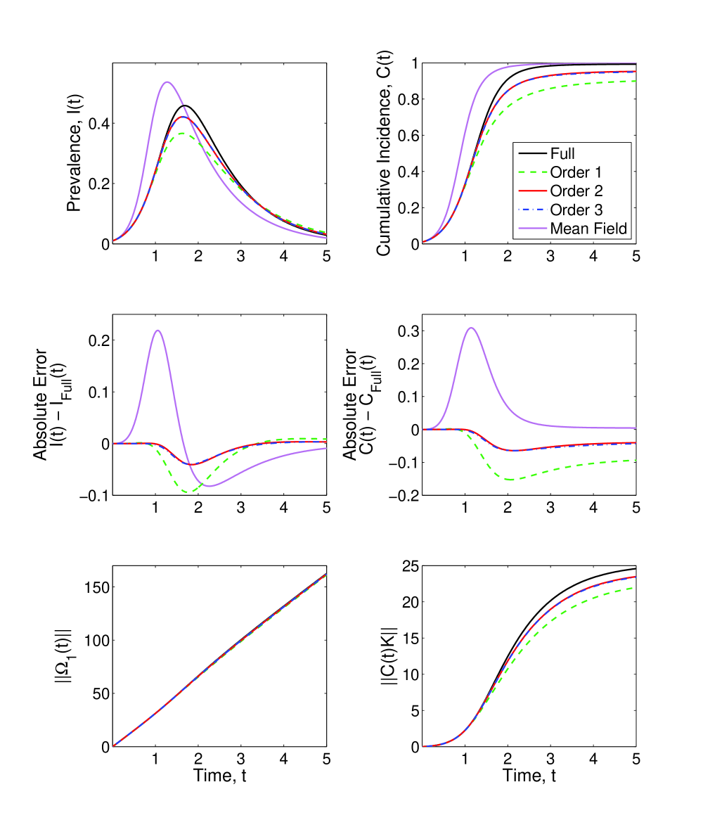
Figure 1: Epidemic dynamics for $n=10$, $\beta=3/2$, $\gamma=1$, $\tau=1/2$ and 1% of the population initially infectious.

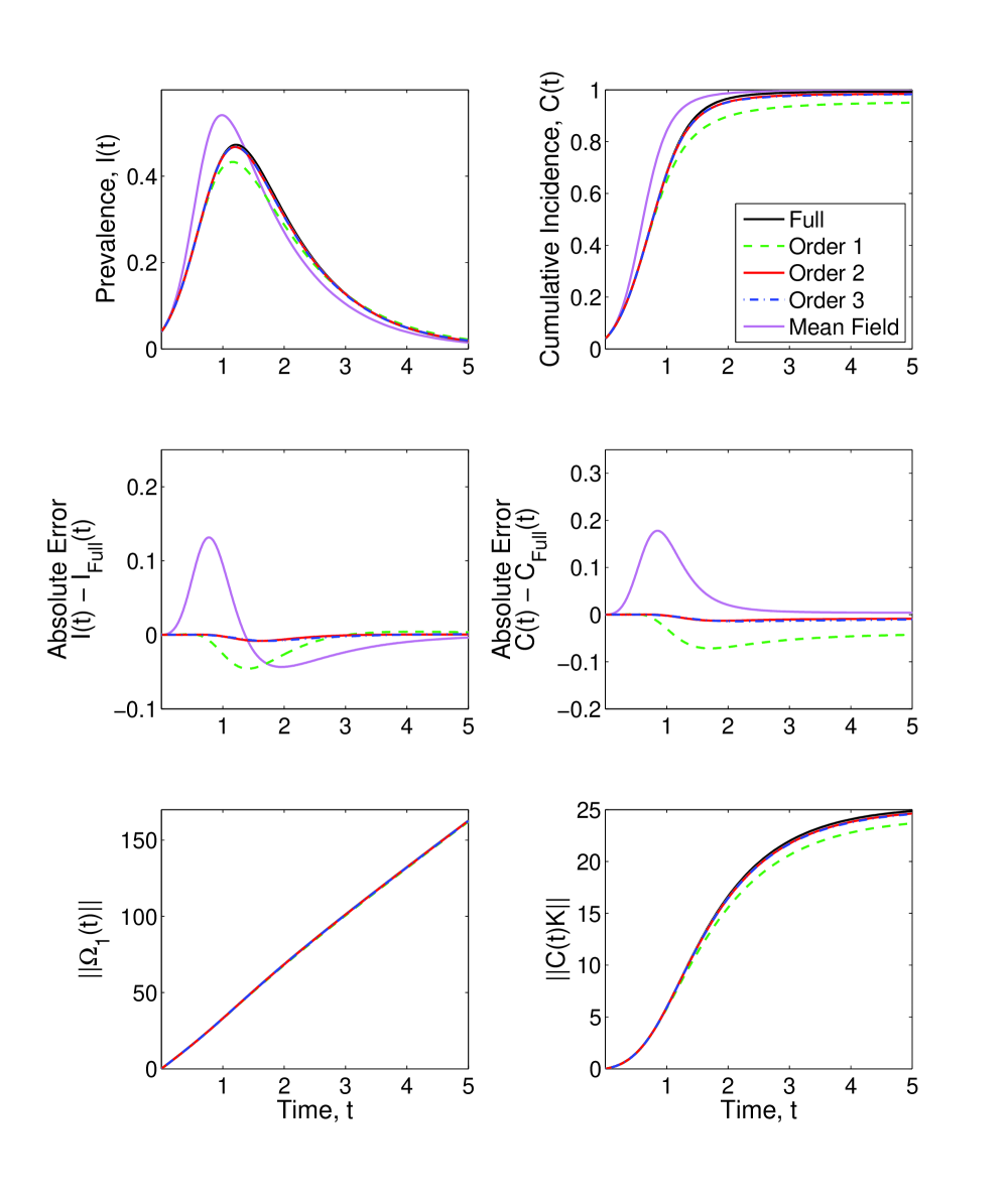
Figure 2: Epidemic dynamics for $n=10$, $\beta=3/2$, $\gamma=1$, $\tau=1/2$ and 4% of the population initially infectious.

For short time periods, the norm $\|\Omega_{1}(t)\|$ is less than the value given in Eq. 7 that is known to be sufficient for convergence of the Magnus series onto the exact solution (Blanes et al., 1998). This value is quickly exceeded, however, and numerical results suggest that while the series does converge, it does so onto something that is not an exact solution to (16), raising the question of how accurate an approximation is obtained. Since there is seldom much difference between the Order 2 and Order 3 systems, we will tend to consider the Order 2 approximation from now on.

Comparing Figures 1 and 2 we see that the agreement between approximation and exact results is very good for initial infectious prevalence of 4%, but not as good for 1% – although in both scenarios the approach clearly outperforms the mean-field model for early times. We can interpret these results in light of the discussion of §3.3 above – if $I(t)$ is too variable over time, we do not expect the approximation to be good since then the solution of (20) is expected to be a further from the solution of (16). The smaller initial condition involves more variability in $I(t)$ over time than the larger, with analogous (but more complex) argumentation holding at higher orders.

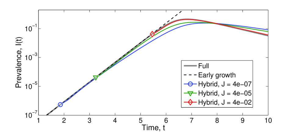
Figure 3: Performance of hybrid approaches for different crossover prevalences $J$, with $n=10$, $\beta=3/2$, $\gamma=1$, $\tau=1/2$.

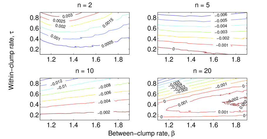
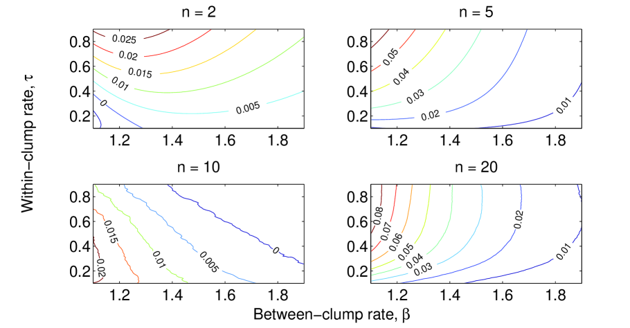
Figure 4: Performance of Order-2 approaches for different values of $n$, $\beta$ and $\tau$, with $\gamma=1$, (top) absolute error in peak (bottom) absolute error in final proportion of the population susceptible.

These observations suggest a hybrid strategy for the SIR model since the behaviour for small levels of infection is a linear dynamical system whose dominant eigenvalue can be calculated efficiently (Ross et al., 2010). Figure 3 shows the results of switching from the early exponential growth rate predicted by the linear system to the Order 2 system at various switchover values of prevalence $J$, demonstrating that we can accurately reduce the problem from 66 to 5 ODEs. Such a strategy could be generalised to other population dynamics where a linear approximation can be used around the fixed points, joined to algebraic methods used when non-linear effects become important.

Finally, Figure 4 shows the behaviour of the Order 2 system over a range of values for $n$, $\tau$ and $\beta$ (since $\gamma$ can be eliminated by a non-dimensionalisation it is not varied). These show that errors remain relatively small, and that the approximation tends to work better for smaller values of $\tau$. This is to be expected, since as $\tau\rightarrow 0$ both the approximation and the full model tend to the standard SIR model.

4 Macroparasite dynamics

Modelling infectious diseases caused by macroparasites such as worms has long been a technical challenge in infectious disease epidemiology (Anderson and May, 1991; Anderson, 1993), with more recent impetus due to the political prioritisation of mitigating neglected tropical diseases (Anderson et al., 2013; Addiss, 2013). Here each person is, from the point of view of worm ecology, a local habitat analogous to the clumps considered above.

Suppose we consider a model of macroparasite dynamics where $p_{w}(t)$ is the proportion of people in the population with a worm burden of $w$. Individuals clear worms at a rate of $d$ per worm, and experience a non-linear force of infection from other infected individuals leading to dynamics

$$\frac{\mathrm{d}}{\mathrm{d}t}{p}_{w}=d(-wp_{w}+(w+1)p_{w+1})+\left({\textstyle\sum_{w^{\prime}}\lambda_{w^{\prime}}p_{w^{\prime}}}\right)(-p_{w}+p_{w-1})\text{ .}$$ (24)

These are a special case of the equations analysed by Isham (1995) using probability generating function and moment closure methods. As before we will write these using vector notation

$$\frac{\mathrm{d}\mathbf{p}}{\mathrm{d}t}=(d\mathbf{D}+\Lambda(t)\mathbf{E})\mathbf{p}\text{ ,}\quad\text{where}\quad\mathbf{p}(t):=(p_{w}(t))\text{ ,}\quad\Lambda(t):=\boldsymbol{\lambda}\cdot\mathbf{p}(t)\text{ ,}\quad\boldsymbol{\lambda}:=(\lambda_{w})\text{ .}$$ (25)

It is then possible to see that the two matrices in this expression are linearly independent and obey $[\mathbf{D},\mathbf{E}]=-\mathbf{E}$. They therefore form a representation of a Lie algebra, meaning we can apply the general methodology of §2.3 above and expand

$$\mathbf{M}(t)=d\mathbf{D}+\Lambda(t)\mathbf{E}\text{ ,}\quad\mathbf{Z}(t)={\delta(t)\mathbf{D}+\varepsilon(t)\mathbf{E}}\text{ ,}\quad\mathbf{G}(t,u)=\Delta(t,u)\mathbf{D}+\mathcal{E}(t,u)\mathbf{E}\text{ .}$$ (26)

Substituting these expansions into (10) gives

$$\frac{\partial\Delta}{\partial u}\mathbf{D}+\frac{\partial\mathcal{E}}{\partial u}\mathbf{E}=\left(\varepsilon(t)\Delta(t,u)-\delta(t)\mathcal{E}(t,u)\right)\mathbf{E}\text{ ,}\quad\Delta(t,0)\mathbf{D}+\mathcal{E}(t,0)\mathbf{E}=\dot{\delta}(t)\mathbf{D}+\dot{\varepsilon}(t)\mathbf{E}\text{ .}$$ (27)

From these equations, together with (4), we obtain a solution

$$\mathbf{p}(t)={\rm e}^{dt\mathbf{D}+\varepsilon(t)\mathbf{E}}\mathbf{p}(0)\text{ ,}\quad\frac{\mathrm{d}\varepsilon}{\mathrm{d}t}=\frac{\Lambda(t)-\varepsilon(t)\eta(t)}{\zeta(t)}\text{ ,}\quad\zeta(t):=\frac{1-{\rm e}^{-dt}}{dt}\text{ ,}\quad\eta(t):=\frac{1-\zeta(t)}{t}\text{ .}$$ (28)

Note that in contrast to the clump-based SIR model, this solution is exact. There are two main benefits of the algebraic approach. First, while traditional moment closures are based on the assumption that $p_{w}$ is the probability mass function for some standard distribution – typically the negative binomial – we know here that the low-parameter form $\mathbf{p}={\rm e}^{\theta_{1}\mathbf{D}+\theta_{2}\mathbf{E}}\boldsymbol{\vartheta}$ holds exactly, giving a similar level of model complexity to the negative binomial while being derived directly from biological mechanisms. Secondly, since $w\in\{0,1,\ldots{}\}$ we must choose a sufficiently large maximum $w$ and keep that fixed to work with (24) directly. In contrast, for (28) we have one ODE and can select whatever maximum value of $w$ is required to secure accurate calculation of the matrix exponential each time step.

5 Discussion

The approximate algebraic method proposed here is not dependent on special features of SIR dynamics, and could be applied to other systems of population dynamics – such as more realistic epidemiological models (e.g. SEIR and SIRS), voter models, or predator-prey systems – provided self-consistent equations like (12) are appropriate. The topology of the network of interactions between individuals also need not be the simplest clump model, and other local-global dynamics – such as the dynamics of House (2010), Volz et al. (2011), and Ma et al. (2013), and potentially dynamics on still more general network structures such as those considered by Karrer and Newman (2010) – can be considered in this framework.

In general, however, the problem of convergence of a matrix series is likely to be the major limitation of algebraic methods – formal convergence is typically too conservative in terms of what will constitute a good approximation. This would motivate derivation of an exact expansion of the kind provided for macroparasite dynamics as in §4 above and elsewhere for other relatively simple kinds of population dynamics (House, 2012; Shang, 2012). At present, the selection of an appropriate linearly independent matrix basis set for more realistic dynamics has not been possible, however hopefully more fundamental approaches to the algebraic treatment of time-inhomogeneous Markov chains such as work by Sumner (2013) will help to provide improved, exact, closures.

References

- Addiss (2013) D. G. Addiss. Epidemiologic models, key logs, and realizing the promise of WHA 54.19. PLoS Neglected Tropical Diseases, 7(2):e2092, 2013.
- Anderson (1993) R. M. Anderson. Chapter 4: Epidemiology. In F. E. G. Cox, editor, Modern Parasitology, pages 75–116. Blackwell Science, 2nd edition, 1993.
- Anderson and May (1991) R. M. Anderson and R. M. May. Infectious Diseases of Humans. Oxford University Press, Oxford, 1991.
- Anderson et al. (2013) R. M. Anderson, J. E. Truscott, R. L. Pullan, S. J. Brooker, and T. D. Hollingsworth. How effective is school-based deworming for the community-wide control of soil-transmitted helminths? PLoS Neglected Tropical Diseases, 7(2):e2027, 02 2013.
- Ball and Neal (2008) F. Ball and P. Neal. Network epidemic models with two levels of mixing. Mathematical Biosciences, 212(1):69–87, 2008.
- Ball et al. (1997) F. Ball, D. Mollison, and G. Scalia-Tomba. Epidemics with two levels of mixing. The Annals of Applied Probability, 7(1):46–89, 1997.
- Blanes et al. (1998) S. Blanes, F. Casas, J. A. Oteo, and J. Ros. Magnus and Fer expansions for matrix differential equations: The convergence problem. Journal of Physics A, 31(1):259–268, 1998.
- Blanes et al. (2002) S. Blanes, F. Casas, and J. Ros. High order optimized geometric integrators for linear differential equations. BIT Numerical Mathematics, 42(2):262–284, 2002.
- Blanes et al. (2013) S. Blanes, F. Casas, J. A. Oteo, and J. Ros. The Fer and Magnus expansions. In B. Engquist et al., editors, Encyclopedia of Applied and Computational Mathematics. Springer, 2013.
- Cornell and Ovaskainen (2008) S. J. Cornell and O. Ovaskainen. Exact asymptotic analysis for metapopulation dynamics on correlated dynamic landscapes. Theoretical Population Biology, 74(3):209–25, 2008.
- Danon et al. (2011) L. Danon, A. P. Ford, T. House, C. P. Jewell, M. J. Keeling, G. O. Roberts, J. V. Ross, and M. C. Vernon. Networks and the epidemiology of infectious disease. Interdisciplinary Perspectives on Infectious Diseases, 2011:1–28, Jan 2011.
- Decreusefond et al. (2012) L. Decreusefond, J.-S. Dhersin, P. Moyal, and V. C. Tran. Large graph limit for a SIR process in random network with heterogeneous connectivity. Annals of Applied probability, 22(2):541–575, 2012.
- Dodd and Ferguson (2007) P. Dodd and N. Ferguson. Approximate disease dynamics in household-structured populations. Journal of The Royal Society Interface, 4(17):1103–1106, 2007.
- Ferguson et al. (2001) N. M. Ferguson, C. A. Donnelly, and R. M. Anderson. The foot-and-mouth epidemic in Great Britain: pattern of spread and impact of interventions. Science, 292(5519):1155–60, 2001.
- Ghoshal et al. (2004) G. Ghoshal, L. M. Sander, and I. M. Sokolov. SIS epidemics with household structure: the self-consistent field method. Mathematical Biosciences, 190(1):71–85, 2004.
- House (2010) T. House. Exact epidemic dynamics for generally clustered, complex networks. arXiv:1006.3483, 2010.
- House (2012) T. House. Lie algebra solution of population models based on time-inhomogeneous Markov chains. Journal of Applied Probability, 49(2):472–481, 2012.
- House and Keeling (2008) T. House and M. J. Keeling. Deterministic epidemic models with explicit household structure. Mathematical Biosciences, 213(1):29–39, 2008.
- House and Keeling (2009) T. House and M. J. Keeling. UK household structure and infectious disease transmission. Epidemiology and Infection, 137(5):654–61, 2009.
- House and Keeling (2010) T. House and M. J. Keeling. The impact of contact tracing in clustered populations. PLoS Computational Biology, 6(3):e1000721, 2010.
- Iserles and Nørsett (1999) A. Iserles and S. P. Nørsett. On the solution of linear differential equations in Lie groups. Philosophical Transactions of the Royal Society, 357(1754):983–1019, 1999.
- Isham (1995) V. Isham. Stochastic models of host-macroparasite interaction. The Annals of Applied Probability, 5(3):720–740, 1995.
- Karrer and Newman (2010) B. Karrer and M. E. J. Newman. Random graphs containing arbitrary distributions of subgraphs. Physical Review E, 82(6):066118, 2010.
- Keeling and Ross (2008) M. Keeling and J. Ross. On methods for studying stochastic disease dynamics. Journal of The Royal Society Interface, 5(19):171–181, 2008.
- Keeling (1999) M. J. Keeling. The effects of local spatial structure on epidemiological invasions. Proceedings of the Royal Society B, 266(1421):859–67, 1999.
- Kirkwood and Boggs (1942) J. G. Kirkwood and E. M. Boggs. The radial distribution function in liquids. Journal of Chemical Physics, 10(6):394–402, 1942.
- Kiss and Simon (2012) I. Z. Kiss and P. L. Simon. New moment closures based on a priori distributions with applications to epidemic dynamics. Bulletin of Mathematical Biology, 74(7):150–1515, 2012.
- Ma et al. (2013) J. Ma, P. Driessche, and F. Willeboordse. Effective degree household network disease model. Journal of Mathematical Biology, 66(1–2):75–94, 2013.
- Magnus (1954) W. Magnus. On the exponential solution of differential equations for a linear operator. Communications on Pure and Applied Mathematics, 7(4):649–673, 1954.
- Miller (2011) J. C. Miller. A note on a paper by Erik Volz: SIR dynamics in random networks. Journal of Mathematical Biology, 62(3):349–358, 2011.
- Miller et al. (2012) J. C. Miller, A. C. Slim, and E. M. Volz. Edge-based compartmental modelling for infectious disease spread. Journal of The Royal Society Interface, 9(70):890–906, 2012.
- Ovaskainen and Cornell (2006) O. Ovaskainen and S. J. Cornell. Space and stochasticity in population dynamics. Proceedings of the National Academy of Sciences, 103(34):12781–12786, 2006.
- Rogers (2011) T. Rogers. Maximum-entropy moment-closure for stochastic systems on networks. Journal of Statistical Mechanics: Theory and Experiment, 2011(05):P05007, 2011.
- Ross (2012) J. V. Ross. On parameter estimation in population models III: Time-inhomogeneous processes and observation error. Theoretical Population Biology, 82(1):1–17, 2012.
- Ross et al. (2010) J. V. Ross, T. House, and M. J. Keeling. Calculation of disease dynamics in a population of households. PLoS ONE, 5:e9666, 2010.
- Shang (2012) Y. Shang. A Lie algebra approach to susceptible-infected-susceptible epidemics. Electronic Journal of Differential Equations, 2012(233):1–7, 2012.
- Sidje (1998) R. B. Sidje. Expokit. A software package for computing matrix exponentials. ACM Transactions on Mathematical Software, 24(1):130–156, 1998.
- Sumner (2013) J. G. Sumner. Lie geometry of Markov matrices. Journal of Theoretical Biology, 327(0):88–90, 2013.
- Taylor et al. (2012) M. Taylor, P. L. Simon, D. M. Green, T. House, and I. Z. Kiss. From Markovian to pairwise epidemic models and the performance of moment closure approximations. Journal of Mathematical Biology, 64(6):1021–1042, 2012.
- Volz (2008) E. M. Volz. SIR dynamics in random networks with heterogeneous connectivity. Journal of Mathematical Biology, 56(3):293–310, 2008.
- Volz et al. (2011) E. M. Volz, J. C. Miller, A. Galvani, and L. Ancel Meyers. Effects of heterogeneous and clustered contact patterns on infectious disease dynamics. PLoS Computational Biology, 7(6):e1002042, 2011.
- Wilcox (1967) R. M. Wilcox. Exponential operators and parameter differentiation in quantum physics. Journal of Mathematical Physics, 8:962–982, 1967.