caption captionlabel

Interactive Chemical Reactivity Exploration

Moritz P. Haag¹, Alain C. Vaucher¹, Maël Bosson², Stéphane Redon^2∗, Markus Reiher^1∗

¹ ETH Zürich, Laboratorium für Physikalische Chemie,

Vladimir-Prelog-Weg 2, CH-8093 Zürich, Switzerland

²NANO-D - INRIA Grenoble - Rhône-Alpes/CNRS Laboratoire Jean Kuntzmann, 655, avenue de l’Europe Montbonnot, 38334 Saint Ismier Cedex, France

Elucidating chemical reactivity in complex molecular assemblies of a few hundred atoms is, despite the remarkable progress in quantum chemistry, still a major challenge. Black-box search methods to find intermediates and transition-state structures might fail in such situations because of the high-dimensionality of the potential energy surface. Here, we propose the concept of interactive chemical reactivity exploration to effectively introduce the chemist’s intuition into the search process. We employ a haptic pointer device with force-feedback to allow the operator the direct manipulation of structures in three dimensions along with simultaneous perception of the quantum mechanical response upon structure modification as forces. We elaborate on the details of how such an interactive exploration should proceed and which technical difficulties need to be overcome. All reactivity-exploration concepts developed for this purpose have been implemented in the Samson programming environment.

$\ast$ Corresponding authors:
S. Redon (stephane.redon@inria.fr) and
M. Reiher (markus.reiher@phys.chem.ethz.ch)

1 Introduction

Unraveling reaction mechanisms on an atomistic level is one of the major goals in quantum chemistry. Reactivity studies require calculations based on the first principles of quantum mechanics to describe the breaking and forming of chemical bonds in a general way not restricted to certain classes of molecules. The algorithmic developments in density functional theory (DFT) and in Hartree–Fock-based electronic structure methods have enabled chemists to calculate the electronic structure of molecular systems up to several hundred atoms with sufficient accuracy and in a reasonable time[1].

A huge effort was made in the past years to allow for the calculation of larger and larger molecules[2, 3, 4]. Despite this success, it is still a major task to explore reaction mechanisms for molecular systems of even medium size (say, one to a few hundred atoms). This is mainly because of the fact that the unsupervised automated exploration of the first-principles potential energy surface (PES) of reactive molecular assemblies is most often prohibitive. The trial-and-error approach currently applied (guessing the important structures and refining them with local optimization methods) requires experience, luck, and time. The need to compose lengthy and at times cryptic text-based input files and to set up large three-dimensional structures with input devices working in only two dimensions like the computer mouse, further hamper a simple and intuitive application.

A more convenient set-up of molecular structures and default values for electronic structure programs is desirable (and in parts available by standard graphical user interfaces). Elegant examples are the structure editors Samson[5] and Avogadro [6]. Nevertheless, it remains a cumbersome procedure to explore reaction mechanisms in systems of a few hundred atoms with two-dimensional input devices and automated search algorithms.

Haptic Quantum Chemistry[7, 8], Interactive Quantum Chemistry[9, 10] and Real-time Quantum Chemistry[11, 12] offer new alternative approaches to study reactivity in large three-dimensional molecular systems by providing an instantaneous response of the system to the structural manipulation.

A so-called haptic pointer device fulfills two functions as an input device and for transmitting the response to the operator. With such a device the operator can perform structure manipulations directly in three dimensions in order to probe the reactivity of a molecular assembly. Then, the response to this probing can be instantaneously presented to the operator as forces rendered by the force-feedback functionality of the device.

In previous work on haptic interaction with molecular systems[13, 14, 15, 16, 17] the rendered forces where obtained from classical force fields or model potentials. As these potentials are not sufficiently general and flexible to account for any kind of bond-breaking event, quantum chemical methods based on the first principles of quantum mechanics are required to calculate the forces.

In this work we present concepts for the intuitive and interactive exploration of chemical reactivity with force-feedback devices. We first describe in section 2 how the operator-driven manipulation of molecular systems takes place in the study of chemical reactivity with haptic pointer devices. This is then followed by an in-depth analysis of problems emerging during such manipulations in section 3. The implementation of these concepts as ‘Apps’ loaded into the Samson environment is then described in section 4. We also present an App to calculate quantum mechanical energies and forces based on the standard non-self-consistent density-functional tight-binding method (DFTB). With this App we are able to describe a larger range of molecules than it is possible with the ASED-MO method provided by Samson. Finally, we summarize our findings and provide an outlook for further extensions and features useful for studying chemical reactivity interactively.

2 Manipulating Molecular Systems with Haptic Pointer Devices

The term ‘manipulation’ of a molecular system shall denote a manual change of atom positions in a molecular assembly. The operator applies structural changes by selecting and moving one or more atoms.

A manipulation creates a sequence of structures that can be interpreted as a path through the configuration space of the molecular assembly. Providing an energy for each structure then creates a reaction energy profile. This one-dimensional profile is a slice through the high-dimensional PES of the system. The goal of chemical reactivity studies is to find (minimum-energy) paths corresponding to the possible reactions of a molecular assembly. They are defined by the steepest-descent path from the transition-state structure to the reactants structure or to the products structure. Starting from a local minimum structure (minimum on the PES) a structural change will result in gradients several (in general, on all) atoms of the system. We may define the set of nuclear gradients as $\{\bm{g}_{I}\}$, where

$$\bm{g}_{I}=\bm{\nabla}_{I}\,E\,\,,$$ (1)

and $I$ refers to a specific atomic nucleus in the assembly. The set of forces $\{\bm{f}_{I}\}$

$$\bm{f}_{I}=-\bm{g}_{I}\,\,,$$ (2)

represents the response of the system (here, exerted on each atom $I$) as a result of a structural change. This primary response will be followed by the secondary response if the structure is allowed to relax by a constrained structure optimization procedure running in the background. Thus, the operator is attracted to local minima of the PES which can help finding minimum energy paths. However, pushing a system on a minimum energy path against a gradient energetically up hill is conceptually not trivial as shall be discussed in this paper.

Haptic pointer devices such as the Phantom Desktop[18] device employed in this work are very intuitive input as well as output devices. They allow the user to manipulate a structure in three dimensions. At the same time, such devices can render the primary force response required to intuitively steer uphill motions and to recognize evasive motions. The structural response is visualized by the rearranging atoms. Haptic pointer devices enable the manipulation of six degrees of freedom, i.e., of position and orientation of only one object at a time — either a single atom or several atoms joined as a rigid body. Only the (net) force corresponding to this object can be rendered. For the presentation of the forces on other atoms force arrows can be displayed (or the operator is forced to switch between atoms or to employ two haptic pointer devices).

2.1 Coupling the Device to Atoms

Before we delve into the scientific aspects of interactive reactivity exploration, we should make a few technical comments on how the device is connected to the molecular events.

An intuitive way to manipulate a molecular system employing a haptic pointer device is to select an atom by positioning the pointer on top of it, clicking a button and then moving the pointer. The atom is then expected to follow the position of the haptic pointer. At every new structure which the operator is generating by moving some of the atoms a new electronic structure (wave function and energy) is optimized and new forces are calculated.

If the atoms are allowed to relax upon the manipulation, the operator’s input and the relaxation procedure need to be combined. This leads to a competing process between the input and the relaxation procedure resulting in the manipulated atoms jumping back and forth. Depending on how often the operator input is adopted during the optimization the active atoms follow more or less closely the input position. The rapid jumps between the position dictated by the input device and the one given by the optimization procedure is, however, problematic, because they can lead to sudden force changes and therefore to an instability in the force rendering.

A more stable scheme is to attach the input device only indirectly to the atoms[19]. This may be achieved by coupling the input device with a spring to the selected atoms. Thereby, we may add an additional force calculated from the distance between the atom position $\bm{r}_{I}$ and the device position $\bm{r}_{\mathrm{device}}$ to the original force $\bm{f}_{I}$ of the selected atom $I$ during the optimization process

$$\bm{f}_{\mathrm{device}}=\bm{f}_{I}+k\,(\bm{r}_{I}-\bm{r}_{\mathrm{device}})\,\,.$$ (3)

The force constant $k$ can be chosen such that the selected atom follows the input device position closely. Still, the manipulated atom position will never be exactly at the position given by the input device. In such a coupling scheme it is more convenient to render the force exerted by the spring than the force of the connected atom. Then, the force felt by the operator is not directly the force that describes the atom’s reactivity.

Such an additional (fictitious) layer thus impairs the intuitive reactivity perception. Therefore, it is desirable to have the input device exactly determining the position of the manipulated atoms. This allows one to have a precise control over the atom positions, which is of paramount importance for the study of the subtle features of PES. In this case, the relaxation procedure is subject to a constraint imposed by the input device as it optimizes only the inactive (not manipulated) part of the molecular assembly.

2.2 Categories of Manipulation

The energy profile of a path described by a structure manipulation in a molecular system may be assigned to one of three dominating idealized shapes. Either a path is going uphill in energy with a positive gradient (modification against a barrier), downhill with a negative gradient (barrier-less modification), or the path is flat with a gradient length of basically zero (neutral modification) as depicted in Figure 1. The latter case also represents the situation at the top of a barrier. We chose the one-dimensional reaction coordinate $\xi$ to be always positive in the direction of progressing manipulation. Then, a positive gradient corresponds to a negative force acting against the direction of manipulation and vice versa.

Figure 1: Manipulations categorized according to the energy path profile. The energy $E$ is plotted along a one-dimensional (collective) reaction coordinate $\xi$. Orthogonal coordinates leading to an energy increase and thus to restoring forces in these directions are not shown.

We define a neutral manipulation as a manipulation by which a property which is part of the response shows no detectable change. This implies, however, that for every property that is presented to the operator a threshold needs to be defined which defines which numerical values of this property are detectable. Note that both the resolution of the rendering and the operator’s ‘sensitivity’ to the targeted sense determine the detectability. In the case of the haptically rendered forces the threshold is determined by the smallest force difference that the human haptic sense can detect. Obviously, one can always magnify differences to such an extent that the operator will eventually see or feel them if deemed useful.

Since neutral manipulations do not involve any change in the gradient or energy, they always start and also end at stable configurations. Such manipulations will occur frequently in the exploration of chemical reactivity, especially at the very beginning of an haptic exploration, if the reactants are far apart from each other. Then, the operator can start by orienting and moving the separated fragments such that they are in some proper starting position for probing the reactivity without experiencing a considerable interaction that would destabilize them.

Usually a reactive exploration begins by following a contra-gradient path, since the vast majority of reaction paths on a PES have a higher lying transition state that needs to be overcome in order to reach the product structure.

3 Two Scales of Reactivity Exploration: Local and Global Exploration

Local minima and the interconnecting first-order saddle points describe the reactivity of many molecular systems sufficiently well according to Eyring’s absolute rate theory[20] — even if they are as large as enzymes[21]. To find, describe, and record them is the aim of reactivity exploration as developed here. This exploration process can be divided into two different parts. The process of finding the structures of reactants and transition states for a network of stable intermediates and reaction paths is what we may call global reactivity exploration. By contrast, exploring a single elementary reaction is in the realm of local reactivity exploration. From the point of view of global reactivity exploration local reactivity exploration is the identification of nodes of the network (local minima) and links between the nodes (transition states). Accordingly, both processes are tightly connected and performed simultaneously.

3.1 Local Reactivity

Local minima mark the start and end points of local reactivity exploration.

Figure 2: Forces acting on a haptic pointer position during a manipulation. The direction of manipulation $\bm{d}$ and four different cases for the forces $\bm{f}$ are shown. (a) The force points parallel in the direction of the manipulation. (b) The force points parallel but in the opposite direction of the manipulation. (c,d) Two different cases with a perpendicular force component.

The intended direction of manipulation $\bm{d}$ (see Figure 2) is a central quantity in the following discussion. This direction is estimated by taking the current velocity of the manipulation. As soon as the configuration leaves a flat area or a minimum point, gradients emerge and the atom controlled by the haptic pointer device experiences a force $\bm{f}$. The projection of the force vector onto the intended direction vector is a useful local descriptor with which one can classify manipulations. If the projection is positive (see Figure 2 c), the manipulation will be a barrier-less modification. If the projection yields a negative value (see Figure 2 d), the force will be repulsive, i.e., the manipulation is against a barrier.

The projection of the force vector $\bm{f}$ onto the intended manipulation direction vector $\bm{d}$ can be further exploited to determine the force components acting parallel,

$$\bm{f}_{\parallel} =\frac{\bm{f}\cdot\bm{d}}{\left|\bm{d}\right|^{2}}\,\bm{d}\,\,,$$ (4)

and perpendicular,

$$\bm{f}_{\perp} =\bm{f}-\bm{f}_{\parallel}\,\,,$$ (5)

with respect to the intended direction. The components can now be monitored during an exploration and they may be scaled independently if deemed useful.

Decisive for the operator’s experience is the magnitude of the perpendicular component. The larger the perpendicular force becomes, the more difficult it is for the operator to continue to persue his/her intended direction. This is, however, not always an unwanted feature. Although it seems to be merely impedimental, important parts of the response are encoded in the perpendicular force component. On the fly, it directs the operator to alternative reaction valleys (minimum energy paths) that are different from the intended one. This feature is welcome as it works against a potential bias of the operator and thus helps to detect unexpected pathways.

Another more technical issue is what we may call the problem of evasive adaptation. It arises solely in manipulations against a barrier. The resistance of the operator to a force response of the system on the manipulated fragment generates an opposing force on all other atoms. In the case of a simultaneously running energy optimization, the molecular system will adapt to the new constraint (that is the fixed atoms) by moving the remaining atoms until the forces on them vanish. If the manipulation is carried out sufficiently slowly so that the system can always adapt, any attempt to overcome a barrier will fail.

Evasive adaptation is a characteristic of the energy optimization procedure that is constantly trying to reach the closest minimum on the PES. A typical example is an addition reaction with a barrier. If the operator pushes a fragment onto another one, the other fragment will simply be pushed away. However, evasive adaptations can also be a useful feature. Assume, for instance, that an operator grabs a fragment by picking one atom to move it in a neutral manipulation. Depending on the movement’s velocity two different events can occur. Either the fragment is torn apart by breaking the weakest bond or the whole fragment just follows the moved atom. The latter can be enforced, if parts of the system are treated as rigid bodies with no internal degrees of freedom but with free overall translation and rotation.

Such artificial constraints mimic a second input device that may keep parts of the system in a suitable position and orientation for the exploration. The energy minimization procedure acts then only on a subspace of the configuration space. The constraints can, of course, also be directly applied by additional haptic devices or other input devices, either operated by the same operator or in a collaborative manner by more than one person. The operator(s) then need(s) to decide when to relax the constraints to avoid exploring artificial reaction paths. The algorithm can provide assistance by rendering (visually or haptically by an additional device) the forces on the constrained fragments. Large forces on single atoms are a clear indication that the corresponding fragment would adapt to a structural manipulation but is hindered by the constraints.

A more general approach is to allow a continuous change between the two scenarios solely based on the speed of the manipulation. For this the quantum chemical structure optimization procedure needs to be adjusted such that a rather slow manipulation of a fragment leads to a translation of the whole fragment and a fast manipulation leads to bond breaking. Then, the operator can intuitively control the behavior without the need of additional devices or other artificial constraints. Fast manipulations with the intention to overcome barriers would then correspond to nonadiabatic manipulations, whereas slow manipulations with an instantaneous structure adaptation would be classified as adiabatic.

If the computational demands of an electronic structure and force calculation (and force evaluation) set an upper limit to the optimization speed, the manipulation has to be slowed down until the optimization is faster than the manipulation. This can be easily achieved by modifying the transformation of the haptic pointer position from the world into the molecular frame.

3.2 Global Reactivity

Exploring global reactivity requires to organize and manage the data obtained during an interactive reactivity exploration and to present it in such a way that the operator quickly obtains an overview. Graphs are a tool to store provisional results of local reactivity studies (see Figure 3). The stored structures are the starting points for further explorations and for the refinement of existing ones. The more structures the operator collects the more the network graph also serves as a tool to organize the results. The operator should be able to change the level of detail for the whole graph, for sub-graphs or even for single pairs of nodes.

In general, the shear number of possible reactions and rearrangements in large assemblies makes it impossible to obtain a simple picture of the system’s entire reactivity. One may aim for a representation of an essential subset of chemical transformations represented as a network of local minima and transition states connected by (elementary) reaction paths. These networks may harbor circles as in catalytic pathways as well as tree-like structures.

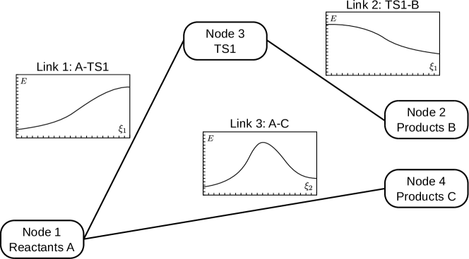
Figure 3: Elements of a reaction network representing the results of a global reactivity exploration. The network shows two reaction paths starting from reactants at Node 1 moving on to the products Nodes 2 and 4. The reaction path from reactants A to products B has already been analyzed as indicated by an additional node (Node 3) corresponding to the transition state TS1. Link 3 shows a link before a closer examination, which would be followed by an extraction of a transition state node and a split of the link. The nodes are arranged according to their energies. Note that Link 1 and 2 belong to the same reaction coordinate ($\xi_{1}$), whereas Link 3 has a different one ($\xi_{2}$)

Collections of molecular structures forming a discretized path through configuration space connect the nodes of the reaction network as links. Optionally, energies and other molecular properties can be stored for each structure of the link, e.g., to provide an energy profile (see insets in Figure 3). Clearly, convenient use of the graph implies that data retrieval (e.g. of structures) is achieved by a single mouse click.

Nodes may be stored automatically when the structure gradient drops below a certain threshold or upon active selection of a structure by the operator. Once a sufficient number of nodes and links is recorded, the operator can analyze the paths in the links. Interesting structures might be marked as entry points for a later exploration.

4 Implementation in the Samson framework

The above outlined features necessary for an interactive study of chemical reactivity have been implemented in a couple of programs (called Apps) that can be loaded into the Samson environment. Since the graphical user interface (GUI) of the Samson program is based on the Qt library [22], Qt classes are heavily used in our Apps, too. For details on the Qt classes employed we refer the reader to the official Qt documentation [22]. In the following, we use the term GUI collectively for all windows, panels, buttons etc. that are part of our Apps.

The density-functional tight-binding (DFTB) App delivers the energies and forces needed for the exploration of molecular reactivity in real time. It implements the standard non-self-consistent variant of DFTB. The functionality for local reactivity studies is split into two separate Apps called Local Reactivity and Phantom Direct. All features concerning the energy minimization and the visual display options are collected in the Local Reactivity App, whereas all features to influence the force rendering and the input behavior of the haptic pointer device are combined in the Phantom Direct App. The global reactivity App is called Global Reactivity Monitoring. It allows the operator to store, organize, and visualize reaction networks, which are the result of reactivity studies as described in the preceding sections.

4.1 DFTB App

In this section, we assess the capabilities of DFTB for interactive reactivity studies. The standard non-self-consistent DFTB method[23, 24] is a highly-parametrized tight-binding method, where all parameters are obtained from DFT calculations and not by fitting them to experimental data.

The DFTB method is based on a Taylor expansion of the DFT energy around a reference electronic density[25], which is a superposition of the atomic densities. It neglects second and higher-order terms and its energy reads

$$E^{\mathrm{DFTB}}=E_{\mathrm{rep}}+\sum_{i}^{\mathrm{occ}}\varepsilon_{i}.$$ (6)

The repulsion energy $E_{\mathrm{rep}}$ is calculated by summing up the pairwise repulsion interactions of the atoms,

$$E_{\mathrm{rep}}=\sum_{I<J}V_{IJ}^{\mathrm{rep}}$$ (7)

The functions $V_{IJ}^{\mathrm{rep}}(R_{IJ})$ are piecewise constructed from analytical functions of the distance $R_{IJ}$ between the atoms $I$ and $J$. They consist of an exponential function at short distances, of third-order polynomials for mid-range distances, and of a fifth-order polynomial that smoothly decreases the repulsion to zero at a given cutoff distance. The coefficients describing these functions are available in parameter sets[26, 27, 28].

The second term on the right hand side of Eq. (6) is the binding energy based on an linear combination of atomic orbitals taking into account only the valence orbitals. It leads to a generalized eigenvalue problem,

$$\bm{H}^{0}\bm{C}=\bm{S}\bm{C}\bm{\varepsilon},$$ (8)

delivering the eigenvector matrix $\bm{C}$ and the diagonal matrix $\bm{\varepsilon}$ containing the single-particle energies $\varepsilon_{i}$. For atomic orbitals $\mu$ and $\nu$ belonging to the same atom, the Hamiltonian matrix elements $H_{\mu\nu}^{0}$ are given by the atomic orbital energies for $\mu=\nu$ and zero for $\mu\neq\nu$. Similarly, the overlap matrix elements for atomic orbitals of the same atom are given by the Kronecker delta. For atomic orbitals belonging to different atoms, the matrix elements $H_{\mu\nu}^{0}$ and $S_{\mu\nu}$ are calculated by performing Slater-Koster transformations[29] of integrals obtained by an interpolation of values tabulated for atom pairs at given distances. These tables are available in the DFTB parameter sets[26, 27, 28].

The force $\bm{f}_{A}$ acting on an atom $A$ is given by the negative gradient of the energy $E^{\mathrm{DFTB}}$ with respect to the corresponding nuclear coordinate[26],

$$\bm{f}_{A}=-\frac{\partial E^{\mathrm{DFTB}}}{\partial{\bm{R}_{A}}}=-\frac{\partial E_{\mathrm{rep}}}{\partial{\bm{R}_{A}}}-\sum_{\mu\nu}\left(P_{\mu\nu}\frac{\partial H_{\mu\nu}^{0}}{\partial{\bm{R}_{A}}}-W_{\mu\nu}\frac{\partial S_{\mu\nu}}{\partial{\bm{R}_{A}}}\right),$$ (9)

where $\bm{P}=\{P_{\mu\nu}\}$ is the density matrix and $\bm{W}=\{W_{\mu\nu}\}$ is the energy-weighted density matrix. As the DFTB method does not involve any integral evaluation and Eq. (8) does not require an iterative solution, the method is computationally inexpensive, which is a considerable advantage for interactive reactivity exploration (if no specialized hardware and parallelism is exploited).

In our implementation, all matrix elements for a given atom pair are calculated in one shot in order to avoid redundant operations and minimize the execution time. The implementation of the interpolation for the matrix elements was inspired by the DFTB+ program[30]. For interatomic distances covered by the tabulated values, an eigth-order interpolation scheme following Neville’s algorithm[31] has been chosen. The matrix elements for interatomic distances larger than the tabulated values are calculated by applying a fifth-order extrapolation that smoothly decreases them to zero. The coefficients for the extrapolation are determined during the initialization of the method. The derivatives of the Hamiltonian and overlap matrix elements are obtained by numerical differentiation of the tabulated values and application of the product and chain rules for the Slater-Koster transformations. For the solution of the generalized eigenvalue problem in Eq. (8), the corresponding function of the Intel${}^{\text{\textregistered}}$ Math Kernel Library[32] has been employed. To dynamically adapt the thickness of bonds rendered by Samson, the Mayer bond-order matrix[33] is calculated from the density and overlap matrices. We applied the MIO[26] and 3OB[27, 28] parameters, designed for organic molecules containing H, C, N, O, P and S atoms. Although these sets were originally developed for the self-consistent-charge DFTB variants DFTB2[26] and DFTB3[34], they yield reasonable molecular structures when we employed them in the non-self-consistent DFTB method. Table 1 shows the execution times for the energy and gradient calculation of a set of test molecules indicating the feasibility of (unparallelized) DFTB for real-time quantum chemical studies on molecules of moderate size.

Table 1: Execution times for the DFTB energy and gradient calculation of different molecular systems. The timings were performed on an Intel${}^{\text{\textregistered}}$ Core${}^{\text{\texttrademark}}$ i7 (3.20 GHz) workstation.

System	Molecular formula	Number of orbitals	Execution time
Methane	CH4	8	< 1 ms
Diels-Alder	C2H4 + C4H6	34	< 1 ms
Parathion	C10H14NO5PS	96	3 ms
Oleic acid	C18H34O2	114	4 ms
Vitamin A	C20H30O	114	4 ms
Endiandric acid C	C23H24O2	124	5 ms
Folic acid	C19H19N7O6	147	7 ms
Cholesterol	C27H46O	152	8 ms
Fexofenadine	C32H39NO4	187	11 ms
Quinovic acid	C30H46O5	186	12 ms
Taxol	C47H51NO14	206	15 ms
NADH	C21H29N7O14P2	215	15 ms
Fullerene	C60	240	20 ms
$\alpha$-Cyclodextrin	C36H60O30	324	31 ms
Vasopressin	C46H65N13O12S2	375	46 ms
Valinomycin	C54H90N6O18	402	54 ms
Tannic acid	C76H52O46	540	95 ms

We assess the reliability of DFTB by comparing it to standard quantum chemical methods. The reference data were obtained with the B3LYP exchange-correlation functional[35, 36, 37] in combination with the aug-cc-pVTZ[38] and def2-TZVP [39] basis sets as well as with the coupled-cluster singles, doubles, and perturbatively treated triples, CCSD(T), approach[40] in combination with the Dunning aug-cc-pVTZ basis set in spin-unrestricted calculations. The results were also compared to the ASED-MO method[41], which is available in Samson[9] and which was applied to demonstrate structure optimization in real time. For ASED-MO, no explicityl optimized parameters for organic compounds are available. The parameters of Ref. [42] were employed in combination with a STO-2G basis[43] for the calculation of the overlap matrix. We note that studying bond breaking processes with standard DFT methods require the breaking of the spin symmetry[44].

Figure 4 displays energy profiles for the breaking of a C-H bond in methane and of the C=O bond in formaldehyde. The energy profile produced by the DFTB method for the C-H bond is in good agreement with the reference DFT calculation. The equilibrium bond length does also not deviate much from the reference value for the C=O bond, but the predicted energy well is too wide. For the haptic exploration of molecular systems, this means that the user feels a too weak force and therefore an inaccurate representation of the stiffness of the carbonyl bond. This inability of the DFTB method to describe polarized systems correctly is well known, since the non-self-consistent character of the method does not allow for charge transfer. Moreover, the DFTB energy profiles exhibits too small dissociation energies. This is not a major drawback as the haptic exploration of the molecular system requires only a qualitatively correct potential energy surface[12]. Figure 4 also shows that the ASED-MO method with the chosen parameters overestimates equilibrium bond lengths. The differences between the molecular structures obtained with DFTB and ASED-MO are illustrated at the example of folic acid in Figure 5. The energy wells predicted by the ASED-MO method are wider and shallower than their DFTB counterparts, which implies easier bond dissociations during the haptic exploration. As every parametrized method, also ASED-MO could be adapted to yield improved bond lengths at the expense of transferability to other systems.

Figure 4: Energy profile for the dissociation of a C-H bond in methane (left) and the C=O bond in formaldehyde (right) as a function of the bond length $d$. At every distance, the remaining coordinates of the system were allowed to relax in order to minimize the energy. The DFTB profiles calculated with the MIO and 3OB parameters for the C-H bond cannot be distinguished except for bond lengths around 1.7 Å. The reference calculations were carried out with the Turbomole program package[45] (version 6.4). Special care has been taken that a truly unrestricted (i.e. broken-spin-symmetry) Kohn–Sham determinant has been converged asymptotically. The energy scale is chosen to be zero for the lowest energy.

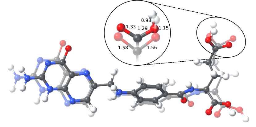
Figure 5: Equilibrium structures of folic acid predicted by the DFTB method (opaque) and the ASED-MO method (partially transparent). The bond lengths in one of the carboxyl groups are indicated in Å in the inset. The bond thickness is an indicator for the calculated Mayer bond order.

Figure 6 shows an energy profile of the Diels-Alder reaction of butadiene and ethene obtained with different methods. The reaction coordinate has been chosen to be the distance between the two parallel lines defined by the two carbon atoms of ethene and the two terminal carbon atoms of butadiene. The DFTB method in combination with the 3OB parameters produces a qualitatively correct energy profile, also compared to previous studies of the reaction[46]. Furthermore, the positions of the energy minimum and maximum are in a good agreement with the B3LYP/def2-TZVP results. The MIO parameters for DFTB and the ASED-MO method fail to reproduce a significant barrier for this reaction pathway. For ASED-MO, a parametrization optimized for this special system might be found that results in a better representation of the barrier.

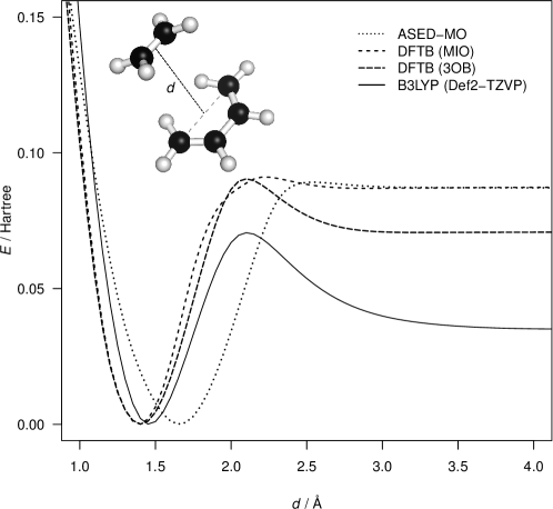
Figure 6: Energy profile for the Diels-Alder reaction between ethene and butadiene. The reaction coordinate is the distance $d$ between the two lines defined by the two carbon atoms of ethene and the two terminal carbon atoms of butadiene, drawn above as a dashed line. At each distance, the structure was allowed to relax while requiring the two lines to remain parallel. The reference calculation was carried out with the Gaussian 09 program package[47] (rev. d.01). The energy scale is shifted to be zero for the lowest energy.

The reactivity of several molecular systems was investigated with DFTB in the Samson framework. The haptic exploration of systems containing less than about 120 atoms proceeds very smoothly. In particular, we observed that the DFTB method allows a remarkably reliable exploration of pericyclic reactions. For example, the biosynthesis of the endiandric acids B and C postulated by Bandaranayake et al.[48], which features a cascade of three pericyclic reactions, could be reproduced correctly using the haptic device. The structures of the reactant, intermediates and products as well as the corresponding energies are given in Figure 7.

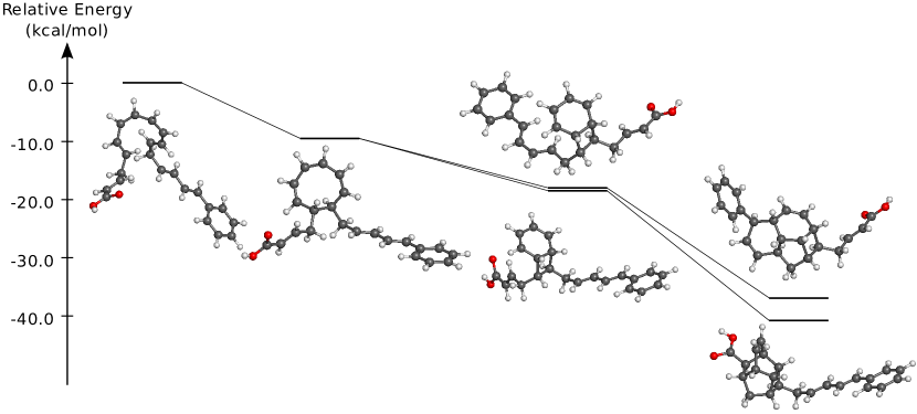
Figure 7: Structures and energies obtained during the exploration of the biosynthesis pathway of endiandric acid B (upper pathway) and C (lower pathway). The first step is an electrocyclic reaction leading to a common intermediate, that undergoes another electrocyclic reaction in the second step, producing one of two possible structures. The third step is in both cases a Diels-Alder reaction.

4.2 Local Reactivity App

The implementation of the local reactivity Apps focuses on the interplay of continuously running loops, whereas the global reactivity App has its focus on the data model developed to store reaction networks. Most of the loops are implemented as functions continuously executed by timers provided by Qt and, thus, are all part of the GUI thread. This implies that these tasks are executed sequentially, which avoids the difficulties that come along with the parallel execution of code. The only exception are tasks which need to communicate with the haptic device. They are executed in a separate thread maintained by the device driver. If the loops, which are part of the GUI thread, become too slow (e.g., for large molecules or more accurate and thus computationally expensive electronic structure calculations), additional threads can be started to allow a parallel execution of the most time demanding tasks. Then, however, the involved data objects need to be made thread-safe. Figure 8 provides an overview over the different loops, threads and their distribution over the two Apps responsible for local reactivity (Local Reactivity App and Phantom Direct App).

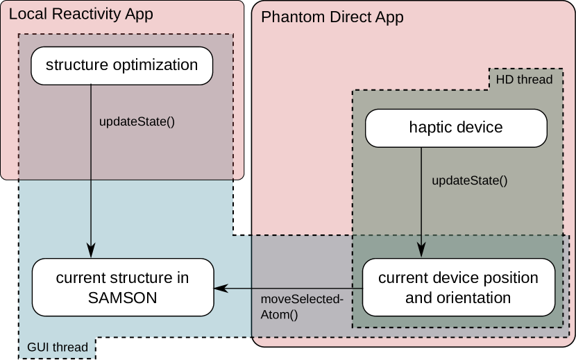
Figure 8: Schematic picture to illustrate the interplay between the GUI thread and the haptic device (HD) thread and the implementation of the loops in the two different local reactivity Apps. The different loops are represented by arrows with the name of the function attached which implements their functionality.

The next step is to choose the algorithm for the energy minimization procedure. Currently we have implemented a steepest descent and a conjugate gradient algorithm. Although the latter is generally more stable and converges faster than the former, in most cases steepest descent will be the method of choice. It has the advantage of always converging to a minimum and of being computationally cheap and therefore fast. More elaborate algorithms will rarely be beneficial in our design of virtual environments (VEs), since during an exploration the configurations to be minimized are always very close to a minimum. However, the modular structure of Samson makes it easy to load other and more complex algorithms such as adaptive integrators[49]. In our steepest descent implementation, the step size and also the number of steps per optimization cycle can be adjusted in a GUI panel that pops up when the algorithm has been selected (see Figure 11 in the appendix). In our studies conducted so far, a step size of $0.02$ and $5$ steps per cycle were sensible start values. Depending on the shape of the PES the step size might need to be adjusted in order to prevent oscillations around the minimum. If it turns out during an exploration that the parameters are not suitable anymore, the parameters as well as the method can be changed on-the-fly.

4.3 Phantom Direct App

With the Phantom Direct App the operator controls the force rendering and is able to adjust all possible scalings that are applied when the molecular force calculated by the electronic-structure method is transformed to the force actually rendered by the device.

The force processing consists of scaling and damping the molecular force to eventually produce the haptic force passed to the device,

$$\bm{f}_{\mathrm{out}}=c(\bm{f}_{\mathrm{in}})\,\bm{f}_{\mathrm{in}}\,\,,$$ (10)

where $c$ may be a function of the force but is subjected to certain conditions. It has to be a strictly positive function of the input force $\bm{f}_{\mathrm{in}}$ and is not allowed to have any zero crossings (apart from the one at the origin), since they would introduce artificial extremal points on the surface[12]. The scaling function chosen for our implementation takes care of the necessary unit conversion and the adaptation of the force range to the range of the haptic device. For details we refer the reader to the corresponding section in the appendix.

A decomposition of the force into components parallel and perpendicular to the intended direction is necessary to scale them separately. As the intended direction, the normalized and damped velocity vector of the end-effector (tip of the “pen” of the haptic device) are taken (the velocity is damped in the same way as the force). The decomposition and scaling will only be performed if the length of the velocity vector is above a certain threshold. The decomposition is carried out as stated in Eqs. (4) and (5). The scaling is then achieved by summing up the components

$$\bm{f}_{\mathrm{h}}=c_{\perp}\bm{f}_{\perp}+c_{\parallel}\bm{f}_{\parallel}\quad\textnormal{with}\quad c_{\perp},c_{\parallel}\geq 0\quad\textnormal{and}\quad c_{\perp}+c_{\parallel}>0\,\,,$$ (11)

where the coefficients $c_{\perp}$ and $c_{\parallel}$ determine the scaling. Because of the conditions for the coefficients, the force direction cannot be rotated by more than 90 degrees, thus assuring that an attractive force never becomes repulsive and vice versa. The condition on the sum (last condition in Eq. (11)) prevents an introduction of artificial zero-crossings.

The molecular input force $\bm{f}_{\mathrm{m}}$ in the simulation loop is updated at a lower frequency than the one in the device loop, since the quantum chemical calculation of the former can hardly be achieved at a kilohertz rate. Thus, we have to apply a damping scheme before the force is passed to the device. This is achieved by calculating the force to be rendered as a superposition

$$\bm{f}^{\mathrm{(h)}}_{\mathrm{m}}=c_{\mathrm{p}}\bm{f}^{\mathrm{(p)}}_{\mathrm{m}}+c_{\mathrm{n}}\bm{f}^{\mathrm{(n)}}_{\mathrm{m}}\quad\textnormal{with}\,\,c_{\mathrm{p}}+c_{\mathrm{n}}=1$$ (12)

of the previously rendered force $\bm{f}^{\mathrm{(p)}}_{\mathrm{m}}$ and the new (scaled) force $\bm{f}^{\mathrm{(n)}}_{\mathrm{m}}$. In our applications, we usually choose $c_{\mathrm{n}}=0.05$ for the damping. The damping not only smoothes the force experience but also prevents fast oscillations when the haptic pointer is trapped in the valley of a steep minimum.

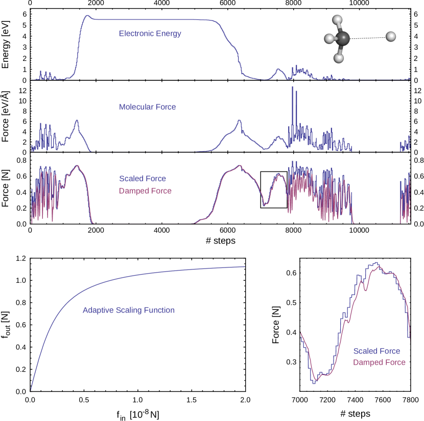
Figure 9: Plots of the electronic energy and the total force magnitudes during exploration of the binding energy of methane (abstraction of a hydrogen atom) employing our non-self-consistent DFTB implementation. The energy and forces have been recorded at every iteration ($\equiv 1\mathrm{step}$) of the device loop. The adaptive scaling was performed as in Eq. (14) with $m=0.5\times 10^{9}\,\mathrm{N}^{-1}$, $f_{\mathrm{max}}=1.2\,\mathrm{N}$. The adaptive scaling function is plotted as a function of the force in Newton, whereas the molecular force is given in $\mathrm{eV}/\text{\AA}$. The adaptively scaled and damped (as in Eq. (12) with $c_{\mathrm{n}}=0.05$) force curves are plotted on top of each other. The bottom right plot magnifies the indicated part in the plot of the scaled and damped force to show the effect of the damping.

The effects of the scaling and damping are illustrated in Figure 9 at the example of the abstraction of a hydrogen atom from a methane molecule. The energy is shifted to be zero for the equilibrium structure of methane. The forces and energies were recorded at every pass of the device loop resulting in $1000$ data points (steps) per second. The plateau occurring roughly between step $2000$ and $5500$ corresponds to the manipulated hydrogen atom being at the dissociation limit. The smaller peaks between step $0$ and step $1000$ and between step $7000$ and step $10000$ are due to distortions from the minimum structure by pulling slowly to allow the relaxation procedure to adapt the positions of the remaining atoms. By this, the operator was actually moving the whole methane molecule. The force curves show the forces calculated by the electronic structure method and illustrate why the adaptive scaling is needed to keep the forces within the range suitable for the device. The very high force peaks are reduced while preserving the subtle differences when the calculated force is comparatively small. From the bottom right plot in Figure 9 one can clearly see that the simulation loop and the device loop are running at different frequency yielding a step function for the rendered force. This is smoothed out by the damping function. The magnified part of the plot shows a possible drawback of the damping. Due to the delay introduced by the damping, force changes that occur at a too high frequency vanish. A too strong damping may lead to artificially flat surfaces by hiding subtle details, but in general, the elimination of high-frequency force changes is wanted. However, in the example shown in Figure 9 the damping does not hide the surface features (force changes) that are characteristic for the reactivity, since they occur at a much lower frequency.

4.4 Global Reactivity Monitoring App

The Global Reactivity Monitoring App serves as a tool to collect, organize, and evaluate the results of a reactivity study. Since stable intermediates and transition state structures are the main result of a reactivity study, the App records and presents them in a graph of the network. Details on the implementation or the data model developed are given in the appendix. A link containing a reaction path can be created by recording a path. This requires that the current molecular structure displayed in Samson corresponds to one node (i.e., one node needs to be active) which will then be the starting node for the link. When the recording is active, the App will react to every structural signal emitted by Samson (every change of an atom position during an exploration leads to a new structural signal) by calculating the RMSD between the current structure and the last recorded structure and adding the new structure as a node to a buffer if the RMSD is above a threshold. When the recording is stopped, a new link is created and the elements of the buffer are moved into the link object. The starting node of the link points to the node that was active at the beginning and the end node is the last node added to the buffer. Both, the start and the end node, are not part of the path, hence are not part of the link. During the recording the energy profile of the reaction path is plotted in the lower panel of the App. At every click on a link that stores a reaction path a window pops up with a more detailed plot of the reaction path, on which the operator can analyze the path by zooming in and out.

New nodes and links can also be added by splitting an existing link with a stored reaction path. The operator can choose a link and specify at which position (which element of the path) the link should be split. The node corresponding to this position will then be promoted to be a top-level item and will be equipped with a corresponding graphics item. Two new links will be created where the new node is the end node of the first and the start node of the second new link. Accordingly, all remaining nodes of the original link up to the new node become part of the first new link and all others part of the second new link.

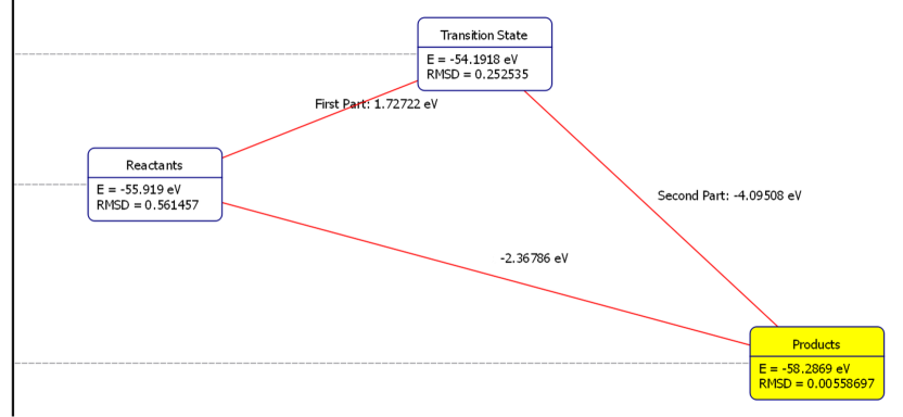
Figure 10: An exemplary reaction network graph in the Global Reactivity Monitoring App is shown. A possible transition state structure has been extracted by splitting the recorded link between the reactants and products nodes. The currently active node is highlighted by the program.

5 Conclusions

The interactive study of chemical reactivity gives rise to new challanges unprecedented in quantum chemistry due to the instantaneous interaction of the operator with the molecular system. To meet them, we started with a careful analysis of the manipulations that the operator applies to the molecular system. The coupling of the haptic (force-feedback) device that is used for the manipulation is decisive for an interactive study of chemical reactivity as the force exerted on an atom of a reactant is the descriptor of reactivity in a reacting molecular system. A transparent and precise control over the atom position is of prime importance in reactivity studies and thus requires a direct coupling of the device to the manipulated atom(s).

We classified the interactive exploration of chemical reactivity as local and global reactivity explorations. For a local reactivity exploration we identified the perpendicular forces and the evasive adaptation behavior as the main problems that may occur during an interactive exploration. The perpendicular forces may make it difficult for the operator to follow a specific path through the configuration space. The evasive adaptation behavior encountered when probing reactivity may hinder the user to reach certain configurations. For both effects, we proposed several schemes that can help to achieve a desired behavior. They include the separate scaling of the perpendicular force component during an exploration and the adaptation of the rate of the continuously running structure optimization.

In the last part of this work, we described an implementation of the ideas developed as Apps that can be loaded into the Samson program environment. They allow the operator to interactively manipulate a molecular system with an haptic device, to study the system’s reactivity, and to deal with difficult scenarios that he/she may encounter.

Our DFTB App is an implementation of the standard non-self-consistent variant of DFTB that allows other Apps in Samson to calculate energies and forces for a given molecular structure. We could show that the DFTB method is an option for the reliable real-time computation of energies and forces for the interactive study of chemical reactivity. It is able to reliably predict molecular structures and to provide a satisfactory description of the reactivity for many molecular systems, while still being fast enough for providing energies and forces in real time. The DFTB method, in combination with the 3OB parameter set, is a useful tool for the haptic exploration of systems containing H, C, N, O, P and S atoms.

The Local Reactivity App together with the Phantom Direct App provide the functionality needed for local reactivity studies. The former enables the operator to control the continuously running structure optimization as well as the interaction with the molecular system with the haptic device. All the necessary parameters can be tuned through a readily accessible graphical user interface.

The functionality of the Global Reactivity Monitoring App allows the operator to easily store, organize and analyze reaction networks. The nodes and links, corresponding to the stable intermediates and the interconnecting reaction paths, are visualized in a reaction network graph. The App allows one to keep track of an ongoing reaction network exploration.

All these Apps extend the Samson program framework to a virtual environment in which chemists are able to intuitively and interactively explore chemical reactivity of molecular systems. It provides all means necessary to interact with the molecular system, obtain the response upon the manipulations and explore the possible reaction paths. Our further development will aim at extending the range of quantum mechanical methods to calculate the energies and forces in real time.

6 Acknowledgment

MPH and MR acknowledge support by ETH Zurich (grant number: ETH-08 11-2). MB and SR acknowledge funding from the European Research Council under the European Union’s Seventh Framework Program (FP/2007-2013) / ERC Grant Agreement n. 307629

Appendix A Technical Peculiarities

As the feasibility of interactive reactivity exploration depends crucially on an efficient implementation, we shall provide these details in this appendix.

A.1 Local Reactivity App

The main task of the Local Reactivity App is to provide access to all parameters necessary to tune the process of the background structure optimization. Additional visual elements such as the display of force vectors can also be switched on. Moreover, in the current version it serves also as an entry point for reactivity studies, as it takes care of all required initialization tasks such as the set up the parameters for the real-time response calculation, which is the electronic structure optimization and the force calculation. The functionality is implemented in the classes SMALocalReactivity and SMALocalReactivityGUI (see Table 2). The corresponding GUI elements are shown in Figure 11.

Table 2: Selection of the classes and their most important members that implemented the functionality of the Local Reactivity App.

class SMALocalReactivity
	updateState()	Calls the structure optimizer which performs a number of optimization cycles specified in the optimizer GUI panel.
	show/hideForces()	Switches the display of the forces on or off.
	updateMonitor()	Updates all the monitoring panels in the GUI.
	addSimulator()	Loads the structure optimizer chosen in the GUI.
	applyInteractionModel()	Loads the interaction model specified in the GUI.
class SMALocalReactivityGUI
	simulationTimer	QTimer object that executes the function optimize() with a frequency given in the GUI (Local Reactivity State Update loop).
	optimize()	Calls SMALocalReactivity::updateState()

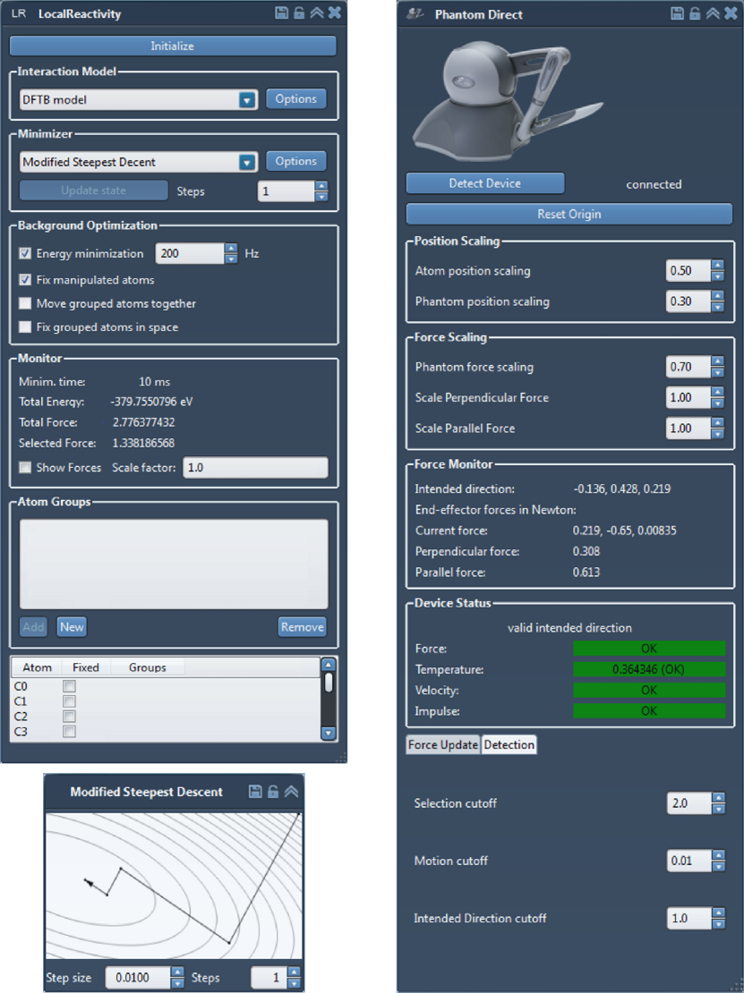
Figure 11: GUI elements for the two Apps devoted to the study of local reactivity. On the left the Local Reactivity App window and the window for adjusting the steepest descent procedure are shown. On the right the window of the Phantom Direct App is presented (the inlay depicts the haptic pointer device).

To start with an interactive exploration the operator needs to specify the particles of the molecular system under study. This is taken care of by the Samson framework, which offers several convenient ways to set up a molecular structure. For instance, the operator can import a Cartesian coordinate file by just pulling it on the main Samson window. A click on “Initialize” internally connects the Local Reactivity App with the molecular structure and sets up the selected electronic structure method for calculating the energy and forces. In the current version the operator can choose between the ASED-MO method [9] and the (non-self-consistent) DFTB implementation reported in this work. They are accessed over a common interface which allows the operator to exchange them by any other interaction model (implemented in a Samson App) that can also provide energies and forces in real time.

With the continuously updated “Monitor” panel the operator can follow some overall properties of the molecular system like the total energy, the magnitude of the total force, and the magnitude of the force on the currently selected atom. Also the forces on all atoms can be displayed as green arrows together with the molecular structure. To be able to detect small residual forces, the force vectors can be scaled. The “Atom Groups” panel allows the operator to define groups of atoms, which can behave as rigid bodies or can be fixed in space. The table at the bottom of the App window provides an overview over all atoms and indicates whether they are fixed or part of a group. It is also possible to directly fix the position of single atoms in this table. These features may help to circumvent the problem of evasive adaptations.

In the “Background Optimization” panel the operator controls the parameters of the structural response calculation. It is possible to start and stop the background energy minimization and to adapt the frequency of its optimization loop. The operator can exclude the manipulated atom from the optimization by fixating it to the position given by the input device. Also, atoms united in a group can be moved together by applying the same displacement to all atoms in the group. Note, however, that this does not necessarily correspond to rigid body movement, since the atoms in the group may relax independently. Also these features may help the operator to avoid unwanted evasive adaptation of the manipulated molecules.

The loop for the background optimization of the molecular structure is implemented in SMALocalReactivity::updateState(), which is indirectly called by the simulationTimer object in the SMALocalReactivityGUI class (see Table 2). The optimizer frequency specified in the GUI is taken to set up the simulationTimer. Since the background optimization loop is part of the GUI thread (see Figure 8), this optimization is not guaranteed to run at the specified frequency. Thus, a frequency below $100\,\mathrm{Hz}$ is unlikely to be realized considering that this already corresponds to an execution every $10\,\mathrm{ms}$ and recalling that the GUI thread is also responsible for processing the events created by all other GUI elements.

A.2 Phantom Direct App

With a click on the “Detect Device” button the device loop is started and a representation of the end-effector position and orientation, the haptic interpoint point (HIP), appears (see Figure 12). To interact with the molecular system the operator has to position the HIP close to an atom and press the device button. If the HIP is close to an atom while the button is pressed the operator can manipulate the atom and simultaneously experiences the force on this atom. Such a situation is depicted in Figure 12 where on the left hand side the HIP representation is shown and on the right hand side the operator is manipulating the position of one atom of the ethene molecule. During the manipulation the “Force Monitor” panel shows the intended direction, the currently rendered force and the force decomposition in the parallel and perpendicular (to the intended direction) component. Additionally, the intended direction is displayed as a turquoise arrow originating from the HIP. If a force is exerted on the manipulated atom, this force is displayed as a red arrow with its origin at the HIP. The overall scaling of the force magnitude and the scaling of the components can be adjusted in the “Force Scaling” panel. The “Position Scaling” panel allows adjusting the scale factors that affect the transformation of the end-effector position to the position of the HIP in the VE. In addition, the operator can adjust several cut-off values for the detection of movements and the atom selection. Also the damping factor for the force update can be modified there.

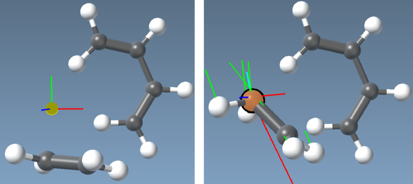
Figure 12: On the left, the molecular structure visualization in Samson and the graphical representation of the HIP (as a yellow ball with three axes) is shown before the operator interacts with the system. On the right, the operator is manipulating an atom (highlighted in orange), which causes the other atoms to rearrange by following their forces (in green). In red, the force experienced by the operator and in turquoise the intended direction of manipulation is depicted.

The cascade of transformations is implemented in the class SMAPhantomConnectorDirect. The parameters for the transformations are taken from the Phantom Direct GUI (see Figure 11 and class SMAPhantomConnectorDirectGUI in Table 3).

Table 3: Selection of the classes and their most important members that implement the functionality of the Phantom Direct App. The haptic interaction point (HIP) is the position of the haptic device (HD) end-effector in the virtual environment.

class SMAPhantomConnectorDirect
	phantomCurrentTransform	Object that stores position and orientation of the end-effector in the world frame.
	detectDevice()	Set up device and start scheduler.
	detectClosestAtom()	Detect if an atom is close to the HIP.
	getPhantomTransformInWorldFrame()	Returns position and orientation of the HIP in the molecular (world) frame.
	moveSelectedAtom()	Move active atom to current HIP position.
	resetOrigin()	Reset origin for the transformation.
	updateState()	Callback function of HD loop.
class SMAPhantomConnectorDirectGUI
	simulationTimer	QTimer object that executes every $10\,\mathrm{ms}$ the function moveSelectedAtom().
	moveSelectedAtom()	Calls moveSelectedAtom() in SMAPhantomConnectorDirect.
class SMAPhantomConnectorDirectHIP
	display()	Executes OpenGL commands to render a sphere and a coordinate system representing position and orientation of the HIP.

The GUI also provides extensive monitoring of the force rendered by the device (in contrast to the molecular force monitored in the Local Reactivity App) and of the haptic device status. The App is specifically designed for the Phantom Desktop device from Sensable Inc [18]. It communicates with the device via an application programming interface (API) that is part of the OpenHaptics${}^{\text{\textregistered}}$ toolkit provided by Sensable [50]. This haptic device API (HDAPI) provides a scheduler that starts a loop in a separate high-priority thread for the communication with the haptic device. This device loop runs at a frequency of $1\,\mathrm{kHz}$ and is responsible for rendering the forces and obtaining the position and orientation of the end-effector (the point corresponding to the tip of the pen-like device). The tasks that read or write the device state are implemented as callback functions registered in the scheduler.

The main functionality of the Phantom Direct App is executed in two simultaneously running loops that are part of two different threads (see Figure 8). The functionality of the App is implemented in the two SMAPhantomConnectorDirect classes (Table 3). The device loop is implemented in the updateState() function called by the device scheduler, whereas the simulation loop is implemented in moveSelectedAtom() called by the simulationTimer. Upon clicking on the “Detect Device” button the detectDevice() function initializes the haptic device and starts the scheduler that handles the device loop. Subsequently the position and orientation of the end-effector is stored as the reference position. This can be also issued by clicking on “Reset Origin” which effectively resets the origin of the haptic device. With scheduling the callback function updateState() the device loop is started. The final steps of the initialization process are to create the visual representation of the HIP in the virtual environment, to enable all user interface elements and to start the simulation loop by calling moveSelectedAtom() for the first time.

The device loop reads the current position and orientation (phantomCurrentTransform) of the device end-effector and sends a force to the device when the operator is manipulating an atom. Unless otherwise stated, the functions and objects accessed from within the loop are also members of the class SMAPhantomConnectorDirect. Figure 13 provides an overview over the procedure executed in updateState() in a flow-chart.

Figure 13: Flow chart of the function SMAPhantomConnectorDirect::updateState() called at every pass of the device loop maintained by the haptic device scheduler.

In the beginning the function determines by reading the state of the device button whether the operator tries to manipulate an atom or whether the device is just moved. If an atom atom is to be moved, detectClosestAtom() will search for an atom within a certain radius around the HIP position. In case of success, a reference to the atom is stored in currentAtom. The next step is to obtain position, orientation and velocity of the end-effector of the haptic device. The velocity is stored in currentVelocity and the phantomCurrentTransform object is updated with the positional and orientational information.

The function getPhantomTransformInWorldFrame() allows us accessing the current position and orientation of the HIP in the reference frame of the VE. In this transformation step the atom position scaling factor is applied. A small factor effectively slows down the movements performed by the operator. As discussed in the preceding sections, this can be exploited to allow for adiabatic manipulations in those cases where the background optimization is not fast enough. A small factor may also help to reduce oscillatory movements due to fast changes in the force direction as they can occur close to steep minima. Only when a force is provided (requires a valid current atom and a valid interaction model) does the function continue with the force processing, otherwise it returns to the scheduler without rendering a force.

The first step in the sequence of transformations is to convert the molecular force into SI units. The forces provided by the interaction model in Samson are in electron volts per Ångström. Since the conversion factor to SI unit

$$1\,\mathrm{eV}\,\text{\AA}^{-1}=1.60218\times 10^{-9}\,\mathrm{N}$$ (13)

is just a constant, it trivially obeys the rules stated above. In the so-called adaptive force scaling step the magnitude of the force vector is adjusted to be in the range which can be rendered by the device. To exploit the given range in an optimal way, small forces are scaled up whereas very high forces are scaled down [51]. This allows the operator to feel the subtle details of an almost flat surface while simultaneously very high forces do not force the operator to perform unwanted movements. An arc tangent function of the form

$$f_{\mathrm{out}}(f_{\mathrm{in}})=\frac{2\,f_{\mathrm{max}}}{\pi}\arctan(m\,f_{\mathrm{in}})$$ (14)

is chosen to scale the magnitude of the force. It is similar to the one chosen in Ref. [51] but ours is of a simpler form involving less parameters. Here, $f_{\mathrm{out}}$ is the force magnitude after the adaptive scaling and $f_{\mathrm{in}}$ is the input force magnitude after the unit conversion. The parameter $f_{\mathrm{max}}$ is the force limit of the device and $m$ determines the “slope” of the function. By adjusting $m$ and $f_{\mathrm{max}}$, one can change the turning point from magnification to reduction (i.e., where the first derivative is $1.0$) of the input force. In Figure 9 (bottom left plot), the graph of this function is shown for suitable parameters applied in our implementation. The strictly monotonically increasing and strictly positive function fulfills our requirements for a conversion function and thus assures that the transformation does not introduce any artificial features into the PES. By only scaling the magnitude of the force, it also does not change the direction of the force vector.

The haptic interaction point is implemented in class SMAPhantomConnectorDirectHIP in the display() function. This function is continuously called by the Samson rendering engine and executes some simple OpenGL commands to render a sphere and three perpendicular axes representing the position and orientation of the HIP (see Figure 12). Position and orientation of the HIP in the correct reference frame are obtained by calling the function getPhantomTransformInWorldFrame().

The actual displacement of an atom, when manipulated by the haptic device, is done in the separate simulation loop (see Figure 8). This separation is necessary, since the device loop runs at a too high frequency. The simulation loop checks whether a manipulation is currently performed and which atom is affected. It reads the position of the HIP by calling the function getPhantomTransformInWorldFrame(). This position is then taken to determine the new position for the atom. In addition to move the selected atom, the simulation loop is responsible for monitoring by updating all GUI monitoring elements.

The functionality of the simulation loop is implemented in the function moveSelectedAtom() of class SMAPhantomConnectorDirect and is triggered by the simulationTimer object (see Table 3). Upon execution, the function performs the following procedure: It starts by checking whether an atom is currently manipulated and, if this is the case, the current position of the atom and the haptic interaction point in the world frame is retrieved. From this, the displacement can be calculated and checked against the specified motion threshold. If the displacement is above the threshold, it is scaled by the atom position scaling factor specified in the GUI and eventually applied to the atom. After that, all user interface elements are updated.

A.3 Global Reactivity Monitoring App

Table 4: Selection of the classes and their most important members that are part of the Global Reactivity Monitoring App.

class SMAGlobalReactivityGUI
	showNetworkView()	Starts the network view.
class GRNetworkView
	_timer	QTimer object that executes every $100\,\mathrm{ms}$ the function updateNetworkElements().
	_model	GRNetworkDataModel objects that stores the data model.
	_graph<View/Scene>	QGraphicsScene and QGraphicsView pair for the graph display.
	updateNetworkElements()	Forces all elements of the data model to update themselves.
	onStructuralSignal()	Reacts to structural changes in case of an active path recording.
	<open/save/$\ldots$>Session()	Functions responsible for session management.
	add<Node/Link>()	Adding a node or link item to the data model stored in _model

The structure of reaction network maps suggests a data model resembling the composite design pattern [52, 163–174] (see Figure 14 and Table 5). The classes storing the data of nodes and the links are called GRNode and GRLink, respectively. GRItem is the common interface from which both classes are derived. It provides all function signatures needed to access the child items of a composite class and to set (and get) the name and the associated graphics object (either GRNodeGraphics or GRLinkGraphics). The graphics objects are responsible for the graphical representation of an item in the graph view. The graph view itself is implemented employing Qt’s QGraphicsView and QGraphicsScene classes which is why the classes GRNodeGraphics and GRLinkGraphics are both derived from QGraphicsItem.

Table 5: Selection of the classes and their most important members that constitute the data model of the Global Reactivity Monitoring App. See also Figure 14 for an overview over all classes.

class GRNetworkDataModel
	rootItem	The invisible root item that has all top-level items as children.
	append<Node/Link>()	Add a top-level node or link item to the data model, i.e., make it a children of rootItem.
	remove<Node/Link>()	Remove a top-level node or link item from the data model, i.e., remove it from rootItem.
	load()/save()	Loading and saving of the data items from and to XML files.
class GRNode
	links()	Get references to all links point to or originating from the node.
	<add/remove>Link()	Register and deregister links.
	setAtoms()/atoms()	Access stored structure snapshot.
	setRmsd()/rmsd()	Access RMSD value.
	setEnergy()/energy()	Access stored energy.
	setActive()/active()	Access activity flag.
	checkStructure()	Determine RMSD value.
	setVector()/vector()	Access vector in configuration space.
class GRLink
	deltaE()	Access energy difference between start and end node.
	setFromNode()/fromNode()	Access start node.
	setToNode()/toNode()	Access end node.
	update()	Determine energy difference and update graphics item.

When the network window is opened the operator starts with an empty graph. The program has, however, already created an invisible (without a graphics object) root item to store the data objects. Upon addition of a new item to the data model the corresponding graphics item is added to the scene. The graphics item is informed about state changes by its data item to keep the graphical representation synchronized with the underlying data model. All items that are visible are stored as direct children of the invisible root item (also called top-level items). The reaction network hierarchy implies the following rules, that are enforced by the implementation:

• GRItems cannot be child of more than one GRItem (including the invisible root item).

• GRLinks can only be top-level items.

• GRNodes can be top-level items (with a graphics item) or part of other top-level items (without a graphics item).

• GRNodes cannot be parents of GRLinks, but of other GRNodes.

Although in principle nodes and links can have GRNodes as children, this feature is currently only implemented for the GRLinks. The children of GRLink items are nodes representing the elements of the path. In contrast to top-level items the GRNodes that are path elements do not have a graphics object.

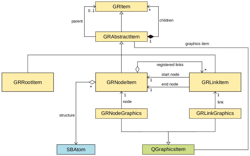
Figure 14: Class diagram for the main components in the global reactivity data model employing the notation defined in the Unified Modeling Language (UML). The classes that are part of the global reactivity data model are yellow, classes from Samson are blue and Qt classes are green. This diagram does not show that GRLinkGraphics in fact derives from QGraphicsPathItem which is in turn derived from QGraphicsItem. GRAbstractItem provides default implementations of the GRItem interface.

The difference between GRNodes and GRLinks manifests in their fields and methods additional to the ones inherited from GRItem. Figure 14 shows that GRLinks and GRNodes are in fact not directly derived from GRItem but from an intermediate abstract class (GRAbstractItem) that provides the default implementation of the functions defined in GRItem.

Every GRNode stores a snapshot of the molecular structure as a collection of SBAtoms (a Samson data type representing atoms). In addition, the nodes update the RMSD between the stored structure and the current structure in Samson. The continuous calculation of the RMSD is again implemented employing a QTimer that forces the items to update their state every $100\,\mathrm{ms}$. Before calculating the RMSD of a node the structure is fitted to the structure in Samson employing a quaternion fit method [53]. This ensures that structures, which differ only in overall orientation and translation, are detected as equal. Based on the RMSD an additional flag is continuously updated which indicates that the structure of the node is equal (within a certain threshold) to the current structure in Samson. Additionally, the energy, a vector representation of the structure, and references to the links connected with the node are stored.

The GRLinks store less information than the GRNodes, since their main information content is the path constituted by their children. They keep references to the nodes where they start and end and save the energy difference between the two nodes.

A node can be created from every structure that is currently active in Samson. The current structure and energy is saved in a new GRNode object, which is then made child of the root item. In addition, a GRNodeGraphics object is created, assigned to the GRNode object and registered, their name can be changed by a double click, and a double click with the middle mouse button sets the current structure in Samson to the structure stored in the node. With this the operator can quickly navigate through the network of nodes and organize it.

The results of a global reactivity session can be stored in the Extensible Markup Language (XML) format. All nodes and links will be stored and can be loaded to continue an already started exploration session. To exchange path elements between different sessions, also single nodes or links can be exported to an XML file and also imported from it. In addition, nodes can also be saved in the xyz file format. This eases the export and import of the structures found from and into other quantum chemistry programs, where they can be refined if deemed necessary.

References

- [1] C. Dykstra, G. Frenking, K. Kim, G. Scuseria, (Eds.), Theory and Applications of Computational Chemistry: The First Forty Years; Elsevier: 2005.
- [2] S. Goedecker, Rev. Mod. Phys. 1999, 71, 1085-1123.
- [3] E. H. Rubensson, E. Rudberg, P. Salek, Methods for Hartree–Fock and Density Functional Theory Electronic Structure Calculations with Linearly Scaling Processor Time and Memory Usage. In Linear-Scaling Techniques in Computational Chemistry and Physics, Vol. 13; R. Zalesny, M. G. Papadopoulos, P. G. Mezey, J. Leszczynski, (Eds.), Springer Netherlands: 2011.
- [4] C. Ochsenfeld, J. Kussmann, D. S. Lambrecht, Linear-Scaling Methods in Quantum Chemistry. In Reviews in Computational Chemistry; John Wiley & Sons, Inc.: 2007.
- [5] M. Bosson, S. Grudinin, X. Bouju, S. Redon, J. Comput. Phys. 2011, 231, 2581-2598.
- [6] M. D. Hanwell, D. E. Curtis, D. C. Lonie, T. Vandermeersch, E. Zurek, G. R. Hutchison, J. Cheminform. 2012, 4, 1-17.
- [7] K. H. Marti, M. Reiher, J. Comput. Chem. 2009, 30, 2010–2020.
- [8] M. P. Haag, K. H. Marti, M. Reiher, ChemPhysChem 2011, 12, 3204-3213.
- [9] M. Bosson, C. Richard, A. Plet, S. Grudinin, S. Redon, J. Comput. Chem. 2012, 33, 779-790.
- [10] M. Bosson, S. Grudinin, S. Redon, J. Comput. Chem. 2013, 34, 492–504.
- [11] M. P. Haag, M. Reiher, Int. J. Quantum Chem. 2013, 113, 8-20.
- [12] M. P. Haag, M. Reiher, Faraday Discuss. 2014, 169, DOI: 10.1039/C4FD00021H, DOI: 10.1039/C4FD00021H.
- [13] F. P. Brooks, Jr., M. Ouh-Young, J. J. Batter, P. Jerome Kilpatrick, SIGGRAPH Comput. Graph. 1990, 24, 177-185.
- [14] A. Křenek, M. Černohorský, Z. Kabelác, Z. Kabeláč, Haptic Visualization of Molecular Model. In WSCG’99 - The 7-th International Conference in Central Europe on Computer Graphics, Visualization and Interactive Digital Media’97, Vol. 1-3; V. Skala, (Ed.), Univ.of West Bohemia Press: 1999.
- [15] E. Harvey, C. Gingold, Haptic representation of the atom. In Information Visualization, 2000. Proceedings. IEEE International Conference on; 2000.
- [16] S. Comai, D. Mazza, A Haptic-Enhanced System for Molecular Sensing. In Human-Computer Interaction — INTERACT 2009, Vol. 5727; T. Gross, J. Gulliksen, P. Kotzé, L. Oestreicher, P. Palanque, R. Prates, M. Winckler, (Eds.), Springer Berlin Heidelberg: 2009.
- [17] R. A. Davies, J. S. Maskery, N. W. John, Chemical Education Using Feelable Molecules. In Proceedings of the 14th International Conference on 3D Web Technology; Web3D ’09 ACM: New York, NY, USA, 2009.
- [18] SensAble Technologies, Inc, “Phantom Desktop Device”, http://www.sensable.com, accessed on 2014/04/14,.
- [19] A. Bolopion, B. Cagneau, S. Redon, S. Régnier, J. Mol. Graph. Model. 2010, 29, 280-289.
- [20] H. Eyring, J. Chem. Phys. 1935, 3, 107–115.
- [21] M. H. Olsson, J. Mavri, A. Warshel, Philos. Trans. R. Soc., B 2006, 361, 1417-1432.
- [22] Digia plc, “Qt Project Reference Pages”, http://qt-project.org/doc/qt-5/reference-overview.html, accessed on 2004/04/14,.
- [23] D. Porezag, T. Frauenheim, T. Köhler, G. Seifert, R. Kaschner, Phys. Rev. B 1995, 51, 12947–12957.
- [24] G. Seifert, D. Porezag, T. Frauenheim, Int. J. Quantum Chem. 1996, 58, 185–192.
- [25] M. Elstner, G. Seifert, Philos. Trans. R. Soc., A 2014, 372,.
- [26] M. Elstner, D. Porezag, G. Jungnickel, J. Elsner, M. Haugk, T. Frauenheim, S. Suhai, G. Seifert, Phys. Rev. B 1998, 58, 7260–7268.
- [27] M. Gaus, A. Goez, M. Elstner, J. Chem. Theory Comput. 2013, 9, 338-354.
- [28] M. Gaus, X. Lu, M. Elstner, Q. Cui, J. Chem. Theory Comput. 2014, 10, 1518-1537.
- [29] J. C. Slater, G. F. Koster, Phys. Rev. 1954, 94, 1498–1524.
- [30] B. Aradi, B. Hourahine, T. Frauenheim, J. Phys. Chem. A 2007, 111, 5678-5684.
- [31] W. Press, B. Flannery, S. Teukolsky, W. Vetterling, Numerical Recipes in C: The Art of Scientific Computing; Cambridge University Press: 1992.
- [32] “Math Kernel Library”, See http://software.intel.com/en-us/articles/intel-mkl.
- [33] I. Mayer, Chem. Phys. Lett. 1983, 97, 270 - 274.
- [34] M. Gaus, Q. Cui, M. Elstner, J. Chem. Theory Comput. 2011, 7, 931-948.
- [35] A. D. Becke, J. Chem. Phys. 1993, 98, 5648-5652.
- [36] C. Lee, W. Yang, R. G. Parr, Phys. Rev. B 1988, 37, 785–789.
- [37] P. J. Stephens, F. J. Devlin, C. F. Chabalowski, M. J. Frisch, J. Phys. Chem. 1994, 98, 11623-11627.
- [38] J. T. H. Dunning, J. Chem. Phys. 1989, 90, 1007-1023.
- [39] F. Weigend, R. Ahlrichs, Phys. Chem. Chem. Phys. 2005, 7, 3297-3305.
- [40] K. Raghavachari, G. W. Trucks, J. A. Pople, M. Head-Gordon, Chem. Phys. Lett. 1989, 157, 479 - 483.
- [41] A. B. Anderson, Int. J. Quantum Chem. 1994, 49, 581-589.
- [42] C. Diaz, F. Mendizabal, Bol. Soc. Chil. Quím. 2001, 46, 293 - 299.
- [43] W. J. Hehre, R. F. Stewart, J. A. Pople, J. Chem. Phys. 1969, 51, 2657-2664.
- [44] C. R. Jacob, M. Reiher, International Journal of Quantum Chemistry 2012, 112, 3661–3684.
- [45] R. Ahlrichs, M. Bär, M. Häser, H. Horn, C. Kölmel, Chem. Phys. Lett. 1989, 162, 165-169.
- [46] S. Sakai, J. Phys. Chem. A 2000, 104, 922-927.
- [47] M. J. Frisch, et al. “Gaussian 09”, Gaussian Inc. Wallingford CT 2009.
- [48] W. M. Bandaranayake, J. E. Banfield, D. S. C. Black, J. Chem. Soc., Chem. Commun. 1980, 19, 902-903.
- [49] R. Rossi, M. Isorce, S. Morin, J. Flocard, K. Arumugam, S. Crouzy, M. Vivaudou, S. Redon, Bioinformatics 2007, 23, i408–i417.
- [50] Sensable Inc, “OpenHaptics Toolkit 3.1 - Programmer’s Guide”, 2012.
- [51] A. Bolopion, B. Cagneau, S. Redon, S. Régnier, Variable gain haptic coupling for molecular simulation. In World Haptics Conference (WHC), 2011 IEEE; 2011.
- [52] E. Gamma, R. Helm, R. Johnson, J. Vlissides, Design Patterns - Elements of Reusable Object-Oriented Software; Addison-Wesley: 2009.
- [53] G. R. Kneller, Mol. Simul. 1991, 7, 113-119.