Optimized Cartesian $K$-Means

Abstract

Product quantization-based approaches are effective to encode high-dimensional data points for approximate nearest neighbor search. The space is decomposed into a Cartesian product of low-dimensional subspaces, each of which generates a sub codebook. Data points are encoded as compact binary codes using these sub codebooks, and the distance between two data points can be approximated efficiently from their codes by the precomputed lookup tables. Traditionally, to encode a subvector of a data point in a subspace, only one sub codeword in the corresponding sub codebook is selected, which may impose strict restrictions on the search accuracy. In this paper, we propose a novel approach, named Optimized Cartesian $K$-Means (OCKM), to better encode the data points for more accurate approximate nearest neighbor search. In OCKM, multiple sub codewords are used to encode the subvector of a data point in a subspace. Each sub codeword stems from different sub codebooks in each subspace, which are optimally generated with regards to the minimization of the distortion errors. The high-dimensional data point is then encoded as the concatenation of the indices of multiple sub codewords from all the subspaces. This can provide more flexibility and lower distortion errors than traditional methods. Experimental results on the standard real-life datasets demonstrate the superiority over state-of-the-art approaches for approximate nearest neighbor search.

1 Introduction

Nearest neighbor (NN) search in large data sets has wide applications in information retrieval, computer vision, machine learning, pattern recognition, recommendation system, etc. However, exact NN search is often intractable because of the large scale of the database and the curse of the high dimensionality. Instead, approximate nearest neighbor (ANN) search is more practical and can achieve orders of magnitude speed-ups than exact NN search with near-optimal accuracy [29].

There has been a lot of research interest on designing effective data structures, such as $k$-d tree [4], randomized $k$-d forest [30], FLANN [22], trinary-projection tree [11, 39], and neighborhood graph search [1, 35, 37, 38].

The hashing algorithms have been attracting a large amount of attentions recently as the storage cost is small and the distance computation is efficient. Such approaches map data points to compact binary codes through a hash function, which can be generally expressed as

$$\mathbf{b}=\mathbf{h}(\mathbf{x})\in\{0,1\}^{L},$$

where $\mathbf{x}$ is a $P$-dimensional real-valued point, $\mathbf{h}(\cdot)$ is the hash function, and $\mathbf{b}$ is a binary vector with $L$ entries. For description convenience, we will use a vector or a code to name $\mathbf{b}$ interchangeably.

The pioneering hashing work, locality sensitive hashing (LSH) [3, 8], adopts random linear projections and the similarity preserving is probabilistically guaranteed. Other approaches based on random functions include kernelized LSH [14], non-metric LSH [21], LSH from shift-invariant kernels [25], and super-bit LSH [10].

To preserve some notion of similarities, numerous efforts have been devoted to finding a good hash function by exploring the distribution of the specific data set. Typical approaches are unsupervised hashing [5, 12, 13, 33, 36, 40, 41, 42] and supervised hashing [16, 23], with kernelized version [7, 17], and extensions to multi-modality [31, 32, 43], etc. Those algorithms usually use Hamming distance, which is only able to produce a few distinct distances, resulting in limited ability and flexibility of distance approximation.

The quantization-based algorithms have been shown to achieve superior performances [9, 24]. The representative algorithms include product quantization (PQ) [9] and Cartesian $K$-means (CKM) [24], which are modified versions of the conventional $K$-means algorithm [19]. The quantization approaches typically learn a codebook $\{\mathbf{d}_{1},\cdots,\mathbf{d}_{K}\}$, where each codeword $\mathbf{d}_{k}$ is a $P$-dimensional vector. The data point $\mathbf{x}$ is encoded in the following way,

$$k^{*}=\arg\min\nolimits_{k\in\{1,2,\cdots,K\}}{\|\mathbf{x}-\mathbf{d}_{k}\|_{2}^{2}},$$ (1)

where $\|\cdot\|_{2}$ denotes the $l_{2}$ norm. The index $k^{*}$ indicates which codeword is the closest to $\mathbf{x}$ and can be represented as a binary code of length $\lceil\log_{2}(K)\rceil$.

The crucial problem for quantization algorithms is how to learn the codebook. In the traditional $K$-means, the codebook is composed of the cluster centers with a minimal squared distortion error. The drawbacks when applying $K$-means to ANN search include that the size of the codebook is quite limited and computing the distances between the query and the codewords is expensive. PQ [9] addresses this problem by splitting the $P$-dimensional space into multiple disjoint subspaces and making the codebook as the Cartesian product of the sub codebooks, each of which is learned on each subspace using the conventional $K$-means algorithm. The compact code is formed by concatenating the indices of the selected sub codeword within each sub codebook. CKM [24] improves PQ by optimally rotating the $P$ dimensional space to give a lower distortion error.

In PQ and CKM, only one sub codeword on each subvector is used to quantize the data points. which results in limited capability of reducing the distortion error and thus limited search accuracy. In this paper, we first present a simple algorithm, extended Cartesian $K$-means (ECKM), which extends CKM by using multiple (e.g., $C$) sub codewords for a data point from the sub codebook in each subspace. Then, we propose the optimized Cartesian $K$-means (OCKM) algorithm, which learns $C$ sub codebooks in each subspace instead of a single sub codebook like ECKM, and selects $C$ sub codewords, each chosen from a different sub codebook. We show that both PQ and CKM are constrained versions of our OCKM under the same code length, which suggests that our OCKM can lead to a lower quantization error and thus a higher search accuracy. Experimental results also validate that our OCKM achieves superior performance.

The remainder of this paper is organized as follows. Related work is first reviewed in Sec. 2. The proposed ECKM is introduced in Sec. 3, followed by the OCKM in Sec. 4. Discussions and experimental results are given in Sec. 5 and 6, respectively. Finally, a conclusion is made in Sec. 7.

2 Related work

Hashing is an emerging technique to represent the high-dimensional vectors as binary codes for ANN search, and has achieved a lot of success in multimedia applications, e.g. image search [6, 15], video retrieval [2, 31], event detection [26], document retrieval [27].

According to the form of the hash function, we roughly categorize the binary encoding approaches as those based on Hamming embedding and on quantization. Roughly, the former adopts the Hamming distance as the dissimilarity between the codes, while the latter does not.

Table I illustrates part of the notations and descriptions used in the paper. Generally, we use the uppercase unbolded symbol as a constant, the lowercase unbolded as the index, the uppercase bolded as the matrix and the lowercase bolded as the vector.

TABLE I: Notations and descriptions.

Symbol	Description
$N$	number of training points
$P$	dimension of training points
$M$	number of subvectors
$S$	number of dimensions on each subvector
$K$	number of (sub) codewords
$m$	index of the subvector
$i$	index of the training point
$\mathbf{R}$	rotation matrix
$\mathbf{D}^{m}$	codebook on $m$-th subvector
$\mathbf{b}^{m}_{i}$	$1$-of-$K$ encoding vector on $m$-th subvector

2.1 Hamming embedding

Linear mapping is one of typical hash functions. Each bit is calculated by

$$h_{i}(\mathbf{x})=\operatorname{sign}(\mathbf{w}_{i}^{T}\mathbf{x}+u_{i}),$$ (2)

where $\mathbf{w}_{i}$ is the projection vector, $u_{i}$ is the offset, and $\operatorname{sign}(z)$ is a sign function which is $1$ if $z>0$, and $0$ otherwise.

Such approaches include  [3, 5, 12]. The differences mainly reside in how to obtain the parameters in the hash function. For example, LSH [3] adopts a random parameter and the similarity is probability preserved. Iterative quantization hashing [5] constructs hash functions by rotating the axes so that the difference between the binary codes and the projected data is minimized.

Another widely-used approach is the kernel-based hash function [7, 13, 14, 17], i.e.

$$h_{i}(\mathbf{x})=\operatorname{sign}(\sum_{j}w_{ij}{\kappa(\mathbf{x},\mathbf{z}_{j})}),$$ (3)

where $\mathbf{z}_{j}$ is the vector in the same space with $\mathbf{x}$, and $\kappa(\cdot,\cdot)$ is the kernel function. The cosine function can also be used to generate the binary codes, such as in [40].

2.2 Quantization

In the quantization-based encoding methods, different constraints on the codeword lead to different approaches, i.e. $K$-Means [18, 19], Product Quantization (PQ) [9] and Cartesian $K$-Means (CKM) [24].

2.2.1 $K$-Means

Given $N$ $P$-dimensional points $\mathcal{X}=\{\mathbf{x}_{1},\cdots,\mathbf{x}_{N}\}\subset\mathbb{R}^{P}$, the $K$-means algorithm partitions the database into $K$ clusters, each of which associates one codeword $\mathbf{d}_{i}\in\mathbb{R}^{P}$. Let $\mathbf{D}=[\mathbf{d}_{1},\cdots,\mathbf{d}_{K}]\subset\mathbb{R}^{P}$ be the corresponding codebook. Then the codebook is learned by minimizing the within-cluster distortion, i.e.

$$\min~{}~{} {\sum_{i=1}^{N}{\|\mathbf{x}_{i}-\mathbf{D}\mathbf{b}_{i}\|_{2}^{2}}}$$

$$\operatorname{s.t.}~{}~{} \mathbf{b}_{i}\in\{0,1\}^{K}$$

$$\|\mathbf{b}_{i}\|_{1}=1~{}~{}i\in\{1,\cdots,N\}$$

where $\mathbf{b}_{i}$ is a $1$-of-$K$ encoding vector ($K$ dimensions with one $1$ and $K-1$ $0$s. ) to indicate which codeword is used to quantize $\mathbf{x}_{i}$, and $\|\cdot\|_{1}$ is the $l_{1}$ norm.

The problem can be solved by iteratively alternating optimization with respect to $\mathbf{D}$ and $\{\mathbf{b}_{i}\}_{i=1}^{N}$ [18].

2.2.2 Product Quantization

One issue of $K$-Means is the size of the codebook is quite limited due to the storage and computational cost. To address the problem, PQ [9] splits each $\mathbf{x}_{i}$ into $M$ disjoint subvectors. Assume the $m$-th subvector contains $S_{m}$ dimensions and then $\sum_{m=1}^{M}{S_{m}}=P$. Without loss of generality, $S_{m}$ is set to $S\triangleq P/M$ and $P$ is assumed to be divisible by $M$. On the $m$-th subvector, $K$-means is performed to obtain $K$ sub codewords. By this method, it generates $K^{M}$ clusters with only $O(KP)$ storage, while $K$-means requires $O(K^{M}P)$ storage with the same number of clusters. Meanwhile, the computing complexity is reduced from $O(K^{M}P)$ to $O(KP)$ to encode one data point.

Let $\mathbf{D}^{m}\in\mathbb{R}^{S\times K}$ be the matrix of the $m$-th sub codebook and each column is a $S$-dimensional sub codeword. PQ can be taken as optimizing the following problem with respect to $\{\mathbf{D}^{m}\}_{m=1}^{M}$ and $\{\mathbf{b}_{i}^{m}\}_{i=1,m=1}^{N,M}$.

$$\begin{split}\min~{}~{}&f_{\text{pq},M,K}=\sum_{i=1}^{N}{\left\|\mathbf{x}_{i}-\begin{bmatrix}\mathbf{D}^{1}\mathbf{b}_{i}^{1}\\ \vdots\\ \mathbf{D}^{M}\mathbf{b}_{i}^{M}\end{bmatrix}\right\|_{2}^{2}}\\ \operatorname{s.t.}~{}~{}&\mathbf{b}_{i}^{m}\in\{0,1\}^{K}\\ &\|\mathbf{b}_{i}^{m}\|_{1}=1~{}~{}i\in\{1,\cdots,N\},m\in\{1,\cdots,M\}\end{split}$$ (4)

where $\mathbf{b}_{i}^{m}$ is also the $1$-of-$K$ encoding vector on the $m$-th subvector and the index of $1$ indicates which sub codeword is used to encode $\mathbf{x}_{i}$.

2.2.3 Cartesian $K$-Means

CKM [24] optimally rotates the original space and formulates the problem as

$$\begin{split}\min~{}~{}&f_{\text{ck},M,K}=\sum_{i=1}^{N}\left\|\mathbf{x}_{i}-\mathbf{R}\begin{bmatrix}\mathbf{D}^{1}\mathbf{b}_{i}^{1}\\ \vdots\\ \mathbf{D}^{M}\mathbf{b}_{i}^{M}\end{bmatrix}\right\|_{2}^{2}\\ \operatorname{s.t.}~{}~{}&\mathbf{R}^{T}\mathbf{R}=\mathbf{I}\\ &\mathbf{b}_{i}^{m}\in\{0,1\}^{K}\\ &\|\mathbf{b}_{i}^{m}\|_{1}=1~{}~{}i\in\{1,\cdots,N\},m\in\{1,\cdots,M\}\end{split}$$ (5)

The rotation matrix $\mathbf{R}$ is optimally learned by minimizing the distortion.

If $\mathbf{R}$ is constrained to be the identity matrix $\mathbf{I}$, it will be reduced to Eqn. 4. Thus, we can assert that under the optimal solutions, we have $f^{*}_{\text{ck},M,K}\leq f^{*}_{\text{pq},M,K}$, where the asterisk superscript indicates the objective function with the optimal parameters.

3 Extended Cartesian $K$-Means

In both PQ and CKM, only one sub codeword is used to encode the subvector. To make the representation more flexible, we propose the extended Cartesian $K$-means (ECKM), where multiple sub codewords can be used in each subspace.

Mathematically, we allow the $l_{1}$ norm of $\mathbf{b}_{i}^{m}$ to be a pre-set number $C$ ($C\geq 1$), instead of limiting it to be exactly 1. Meanwhile, any entry of $\mathbf{b}_{i}^{m}$ is relaxed as a non-negative integer instead of a binary value. The formulation is

$$\begin{split}\min~{}~{}&f_{\text{eck},M,K,C}=\sum_{i=1}^{N}\left\|\mathbf{x}_{i}-\mathbf{R}\begin{bmatrix}\mathbf{D}^{1}\mathbf{b}_{i}^{1}\\ \vdots\\ \mathbf{D}^{M}\mathbf{b}_{i}^{M}\end{bmatrix}\right\|_{2}^{2}\\ \operatorname{s.t.}~{}~{}&\mathbf{R}^{T}\mathbf{R}=\mathbf{I}\\ &\mathbf{b}_{i}^{m}\in\mathbb{Z}_{+}^{K}\\ &\|\mathbf{b}_{i}^{m}\|_{1}=C\end{split}$$ (6)

where $\mathbb{Z}_{+}$ denotes the set of non-negative integers. The constraint is applied on all the points $i\in\{1,\cdots,N\}$ and on all the subspaces $m\in\{1,\cdots,M\}$. In the following, we omit the range of $i,m$ without confusion.

For the $m$-th sub codebook $\mathbf{D}^{m}\in\mathbb{R}^{S\times K}$, traditionally only one sub codeword can be selected and there are only $K$ choices to encode the $m$-th subvector of $\mathbf{R}^{T}\mathbf{x}_{i}$. In the extended version, any feasible $\mathbf{b}_{i}^{m}$ satisfying $\mathbf{b}_{i}^{m}\in\mathbb{Z}_{+}^{K}$ and $\|\mathbf{b}_{i}^{m}\|_{1}=C$ constructs a quantizer, i.e. $\mathbf{D}^{m}\mathbf{b}_{i}^{m}$. Thus, the total number of choices is $\binom{K+C-1}{K-1}\geq K$. For example with $K=256$ and $C=2$, the difference is $\binom{K+C-1}{K-1}=32896\gg K=256$. With a more powerful representation, the distortion errors can be potentially reduced.

In theory, $\log_{2}\binom{K+C-1}{K-1}$ bits can be used to encode one $\mathbf{b}_{i}^{m}$, and the code length is $M\log_{2}(\binom{K+C-1}{K-1})$. Practically, we use $\log_{2}(K)$ bits to encode one position of $1$. The $l_{1}$ norm of $\mathbf{b}_{i}^{m}$ is $C$, which can be interpreted that there are $C$ $1$s in $\mathbf{b}_{i}^{m}$. Then $MC\log_{2}(K)$ bits are allocated to encode one data point.

3.1 Learning

Similar to [24], we present an iterative coordinate descent algorithm to solve the problem in Eqn. 6. There are three kinds of unknown variables, $\mathbf{R}$, $\mathbf{D}^{m}$, and $\mathbf{b}_{i}^{m}$. In each iteration, two of them are fixed, and the other one is optimized.

3.1.1 Solve $\mathbf{R}$ with $\mathbf{b}_{i}^{m}$ and $\mathbf{D}^{m}$ fixed

With

$$\mathbf{X} \triangleq\begin{bmatrix}\mathbf{x}_{1}&\cdots&\mathbf{x}_{N}\end{bmatrix}$$

$$\mathbf{D} \triangleq\begin{bmatrix}\mathbf{D}^{1}&&\\ &\ddots&\\ &&\mathbf{D}^{M}\end{bmatrix}$$

$$\mathbf{B} \triangleq\begin{bmatrix}\mathbf{b}_{1}&\cdots&\mathbf{b}_{N}\end{bmatrix}$$

$$\mathbf{b}_{i} \triangleq\begin{bmatrix}{\mathbf{b}_{i}^{1}}^{T}&\cdots&{\mathbf{b}_{i}^{M}}^{T}\end{bmatrix}^{T},$$

we re-write the objective function of Eqn. 6 in a matrix form as

$$\|\mathbf{X}-\mathbf{R}\mathbf{D}\mathbf{B}\|_{F}^{2},$$

where $\|\cdot\|_{F}$ is the Frobenius norm. The problem of solving $\mathbf{R}$ is the classic Orthogonal Procrustes problem [28] and the solution can be obtained as follows: if SVD of $\mathbf{X}{(\mathbf{D}\mathbf{B})}^{T}$ is $\mathbf{X}{(\mathbf{D}\mathbf{B})}^{T}=\mathbf{U}\Sigma\mathbf{V}^{T}$, the optimal $\mathbf{R}$ will be $\mathbf{U}\mathbf{V}^{T}$.

3.1.2 Solve $\mathbf{D}^{m}$ with $\mathbf{b}_{i}^{m}$ and $\mathbf{R}$ fixed

Let $\mathbf{z}_{i}\triangleq\mathbf{R}^{T}\mathbf{x}_{i}$ and the $m$-th subvector of $\mathbf{z}_{i}$ be $\mathbf{z}_{i}^{m}$. The objective function of Eqn. 6 can also be written as,

$$\sum_{i=1}^{N}\sum_{m=1}^{M}{\|\mathbf{z}_{i}^{m}-\mathbf{D}^{m}\mathbf{b}_{i}^{m}\|_{2}^{2}}=\sum_{m=1}^{M}\|\mathbf{Z}^{m}-\mathbf{D}^{m}\mathbf{B}^{m}\|_{F}^{2},$$ (7)

where

$$\mathbf{Z}^{m} \triangleq[\mathbf{z}_{1}^{m},\cdots,\mathbf{z}_{N}^{m}]$$

$$\mathbf{B}^{m} \triangleq[\mathbf{b}_{1}^{m},\cdots,\mathbf{b}_{N}^{m}].$$

Each $\mathbf{D}^{m}$ can be individually optimized as $(\mathbf{Z}^{m}{\mathbf{B}^{m}}^{T})(\mathbf{B}^{m}{\mathbf{B}^{m}}^{T})^{+}$, where $(\cdot)^{+}$ denotes the matrix (pseudo)inverse.

3.1.3 Solve $\mathbf{b}_{i}^{m}$ with $\mathbf{D}^{m}$ and $\mathbf{R}$ fixed

From Eqn. 6 and Eqn. 7, $\mathbf{b}_{i}^{m}$ can be solved by optimizing

$$\min~{}~{} g_{\text{eck}}(\mathbf{b}_{i}^{m})=\|\mathbf{z}_{i}^{m}-\mathbf{D}^{m}\mathbf{b}_{i}^{m}\|_{2}^{2}$$

$$\operatorname{s.t.}~{}~{} \mathbf{b}_{i}^{m}\in\mathbb{Z}_{+}^{K}$$

$$\|\mathbf{b}_{i}^{m}\|_{1}=C$$

This is an integer quadratic programming and challenging to solve. Here, we present a simple but practically efficient algorithm, based on matching pursuit [20] and illustrated in Alg. 1. In each iteration, we hold a residual variable $\mathbf{r}$, initialized by $\mathbf{z}_{i}^{m}$ (Line 2 in Alg. 1). Let $\mathbf{d}_{k}^{m}$ be the $k$-th column of $\mathbf{D}^{m}$. Each column is scanned to obtain the best one to minimize the distortion error (Line 4), i.e.

$$k^{*}=\arg\min_{k}{\|\mathbf{r}-\mathbf{d}_{k}^{m}\|_{2}^{2}}.$$

Then $\mathbf{r}$ is subtracted by $\mathbf{d}_{k^{*}}^{m}$ (Line 5) for the next iteration, and the $k^{*}$-th dimension of $\mathbf{b}_{i}^{m}$ increases by $1$ (Line 6) to indicate the $k^{*}$-th sub codeword is selected. The process stops until $C$ iterations are reached.

Algorithm 1 Code Generation for ECKM

0:  $\mathbf{z}_{i}^{m}$, $\mathbf{D}^{m}\in\mathbb{R}^{S\times K}$, $C$

0:  $\mathbf{b}_{i}^{m}$

1:  $\mathbf{b}_{i}^{m}=\text{zeros}(K,1)$

2:  $\mathbf{r}=\mathbf{z}_{i}^{m}$

3:  for $c=1:C$ do

4:     $k^{*}=\arg\min_{k}{\|\mathbf{r}-\mathbf{d}_{k}^{m}\|_{2}^{2}}$

5:     $\mathbf{r}=\mathbf{r}-\mathbf{d}_{k^{*}}^{m}$

6:     ${b}_{i}^{m}(k^{*})={b}_{i}^{m}(k^{*})+1$

7:  end for

4 Optimized Cartesian $K$-Means

Before introducing the proposed OCKM, we first present another equivalent formulation of the ECKM. Since each entry of $\mathbf{b}_{i}^{m}$ in Eqn. 6 is a non-negative integer, and the sum of all the entries is $C$, we replace it by

$$\mathbf{b}_{i}^{m}=\sum_{c=1}^{C}{\mathbf{b}_{i}^{m,c}}$$ (8)

with

$$\begin{split}&\mathbf{b}_{i}^{m,c}\in\{0,1\}^{K}\\ &\|\mathbf{b}_{i}^{m,c}\|_{1}=1.\end{split}$$ (9)

Given any feasible $\mathbf{b}_{i}^{m}$, we can always find at least one group of $\{\mathbf{b}_{i}^{m,c}\}_{c=1}^{C}$ satisfying Eqn. 9 and Eqn. 8. Any group of $\{\mathbf{b}_{i}^{m,c}\}_{c=1}^{C}$ satisfying Eqn. 9 can also construct a valid $\mathbf{b}_{i}^{m}$ by Eqn. 8 for Eqn. 6. For example, if $\mathbf{b}_{i}^{m}=\begin{bmatrix}2&0&1&0\end{bmatrix}$, we can replace it by the summation of $\begin{bmatrix}1&0&0&0\end{bmatrix}$, $\begin{bmatrix}1&0&0&0\end{bmatrix}$ and $\begin{bmatrix}0&0&1&0\end{bmatrix}$.

Substituting Eqn. 8 into the objective function of Eqn. 6, we have

$$f_{\text{eck},M,K,C}=\sum_{i=1}^{N}{\left\|\mathbf{x}_{i}-\mathbf{R}\begin{bmatrix}\sum_{c}{\mathbf{D}^{1}\mathbf{b}_{i}^{1,c}}\\ \vdots\\ \sum_{c}{\mathbf{D}^{M}\mathbf{b}_{i}^{M,c}}\end{bmatrix}\right\|_{2}^{2}}.$$

On the $m$-th subvector, $\mathbf{b}_{i}^{m,c}$ represents the selected sub codeword. There are in total of $C$ selections from a single sub codebook. To further reduce the distortion errors, we propose to expand one sub codebook to $C$ different sub codebooks $\mathbf{D}^{m,c}\in\mathbb{R}^{S\times K},c\in\{1,\cdots,C\}$, each of which is used for sub codeword selection. In summary, the formulation is as follows.

$$\begin{split}\min&f_{\text{ock},M,K,C}=\sum_{i=1}^{N}{\left\|\mathbf{x}_{i}-\mathbf{R}\begin{bmatrix}\sum_{c}{\mathbf{D}^{1,c}\mathbf{b}_{i}^{1,c}}\\ \vdots\\ \sum_{c}{\mathbf{D}^{M,c}\mathbf{b}_{i}^{M,c}}\end{bmatrix}\right\|_{2}^{2}}\\ \operatorname{s.t.}&~{}\mathbf{R}^{T}\mathbf{R}=\mathbf{I}\\ &~{}\mathbf{b}_{i}^{m,c}\in\{0,1\}^{K}\\ &~{}\|\mathbf{b}_{i}^{m,c}\|_{1}=1\end{split}$$ (10)

which we call Optimized Cartesian $K$-Means (OCKM).

Since any $\mathbf{b}_{i}^{m,c}$ requires $\log_{2}(K)$ bits to encode, the code length of representing each point is $MC\log_{2}(K)$.

4.1 Learning

Similar with ECKM, an iterative coordinate descent algorithm is employed to optimize $\mathbf{R}$, $\mathbf{D}^{m,c}$ and $\mathbf{b}_{i}^{m,c}$.

4.1.1 Solve $\mathbf{R}$ with $\mathbf{D}^{m,c}$ and $\mathbf{b}_{i}^{m,c}$ fixed

The objective function is re-written in a matrix form as

$$\|\mathbf{X}-\mathbf{R}\hat{\mathbf{D}}\hat{\mathbf{B}}\|_{F}^{2},$$

where

$$\hat{\mathbf{D}} \triangleq\begin{bmatrix}\hat{\mathbf{D}}^{m}&&\\ &\ddots&\\ &&\hat{\mathbf{D}}^{m}\end{bmatrix}$$ (11)

$$\hat{\mathbf{D}}^{m} \triangleq\begin{bmatrix}\mathbf{D}^{m,1}&\cdots&\mathbf{D}^{m,C}\end{bmatrix}$$ (12)

$$\hat{\mathbf{B}} \triangleq\begin{bmatrix}{{}\hat{\mathbf{B}}^{1}}^{T}&\cdots&{{}\hat{\mathbf{B}}^{M}}^{T}\end{bmatrix}^{T}$$ (13)

$$\hat{\mathbf{B}}^{m} \triangleq\begin{bmatrix}\hat{\mathbf{b}}_{1}^{m}&\cdots&\hat{\mathbf{b}}_{N}^{m}\end{bmatrix}$$ (14)

$$\hat{\mathbf{b}}_{i}^{m} \triangleq\begin{bmatrix}{\mathbf{b}_{i}^{m,1}}^{T}&\cdots&{\mathbf{b}_{i}^{m,C}}^{T}\end{bmatrix}^{T}.$$ (15)

Then optimizing $\mathbf{R}$ is the Orthogonal Procrustes Problem [28].

4.1.2 Solve $\mathbf{D}^{m,c}$ with $\mathbf{R}$ and $\mathbf{b}_{i}^{m,c}$ fixed

Similar with Eqn. 7 in ECKM, the objective function of OCKM can be written as

$$\sum_{m=1}^{M}{\|\mathbf{Z}^{m}-\hat{\mathbf{D}}^{m}\hat{\mathbf{B}}^{m}\|_{F}^{2}}.$$

Each $\hat{\mathbf{D}}^{m}$ can also be individually solved by the matrix (pseudo)inversion.

4.1.3 Solve $\mathbf{b}_{i}^{m,c}$ with $\mathbf{R}$ and $\mathbf{D}^{m,c}$ fixed

The sub problem is

$$\min~{}~{} g_{\text{ock}}(\hat{\mathbf{b}}_{i}^{m,c})=\|\mathbf{z}_{i}^{m}-\sum_{c=1}^{C}{\mathbf{D}^{m,c}\mathbf{b}_{i}^{m,c}}\|_{2}^{2}$$

$$\operatorname{s.t.}~{}~{} \mathbf{b}_{i}^{m,c}\in\{0,1\}^{K}$$

$$\|\mathbf{b}_{i}^{m,c}\|_{1}=1$$

One straightforward method to solve the sub problem is to greedily find the best sub codeword in $\mathbf{D}^{m,c}$ one by one similar with Alg. 1 for ECKM. One drawback is the succeeding sub codewords can only be combined with the previous one sub codeword.

Algorithm 2 Code generation for OCKM

0:  $\mathbf{z}_{i}^{m}$, $\hat{\mathbf{D}}^{m}\in\mathbb{R}^{S\times KC}$

0:  $\hat{\mathbf{b}}_{i}^{m}$

1:  [$\hat{\mathbf{b}}_{i}^{m}$, error] = GenCodeOck($\mathbf{z}_{i}^{m}$, $\hat{\mathbf{D}}^{m}$, 1)

Algorithm 3 [$\hat{\mathbf{b}}$, error] = GenCodeOck($\mathbf{z}_{i}^{m}$, $\hat{\mathbf{D}}^{m}$, idx)

1:  if $\text{idx}==\text{C}$ then

2:     $k^{*}=\arg\min_{k}{\|\mathbf{z}-\mathbf{d}_{k}^{m,\text{idx}}\|_{2}^{2}}$

3:     $\mathbf{b}=\text{zeros}(K,1)$

4:     ${b}(k^{*})=1$

5:     $\text{error}=\|\mathbf{z}-\mathbf{d}^{m,\text{idx}}_{k^{*}}\|_{2}^{2}$

6:  else

7:     $[k^{*}_{1},\cdots,k^{*}_{T}]=\arg\min_{k}{\|\mathbf{z}_{i}^{m}-\mathbf{d}_{k}^{m,\text{idx}}\|_{2}^{2}}$

8:     $\text{best}.\text{error}=\text{LARGE}$

9:     for $i=1:T$ do

10:        $k\leftarrow k_{i}^{*}$

11:        $\mathbf{z}^{\prime}=\mathbf{z}_{i}^{m}-\mathbf{d}_{k}^{m,\text{idx}}$

12:        [$\hat{\mathbf{b}}^{\prime}$, $\text{error}^{\prime}$] = GenCodeOck($\mathbf{z}^{\prime}$, $\hat{\mathbf{D}}^{m}$, $\text{idx}+1$)

13:        if $\text{error}^{\prime}<\text{best}.\text{error}$ then

14:           $\text{best}.\text{error}=\text{error}^{\prime}$

15:           $\text{best}.\text{idx}=k$

16:           $\text{best}.\hat{\mathbf{b}}=\hat{\mathbf{b}}^{\prime}$

17:        end if

18:     end for

19:     $\mathbf{b}^{1}=\text{zero}(K,1)$

20:     ${b}^{1}(\text{best}.\text{idx})=1$

21:     $\hat{\mathbf{b}}=[\mathbf{b}^{1};\text{best}.\hat{\mathbf{b}}]$

22:  end if

To increase the accuracy with a reasonable time cost, we improve it as multiple best candidates matching pursuit. The algorithm is illustrated in Alg. 2 and Alg. 3. The input is the target vector $\mathbf{z}_{i}^{m}$, and the sub codebooks $\hat{\mathbf{D}}^{m}$ (defined in Eqn. 12). The output is the binary code represented as $\hat{\mathbf{b}}_{i}^{m}$ (defined in Eqn. 15).

The function $[\hat{\mathbf{b}},\text{error}]=\text{GenCodeOck}(\mathbf{z}_{i}^{m},\hat{\mathbf{D}}^{m},\text{idx})$ in Alg. 3 encodes $\mathbf{z}_{i}^{m}$ with the last $(C-\text{idx}+1)$ sub codebooks $\{\mathbf{D}^{m,c},c\in\{\text{idx},\cdots,C\}\}$. The encoding vector $\hat{\mathbf{b}}$ with $(C-\text{idx}+1)K$ dimensions and the distortion error are returned.

At first, $\text{idx}=1$ and we search the top-$T$ best columns in $\mathbf{D}^{m,\text{idx}}$ (Line 7 in Alg. 3) with $T$ being a pre-defined parameter. Let $\mathbf{d}_{k}^{m,\text{idx}}$ be the $k$-th column of $\mathbf{D}^{m,\text{idx}}$. The final selected one is taken among the $T$ best candidates. For each candidate, the target vector is substracted by the corresponding sub codeword (Line 11), and then the rest codes $\hat{\mathbf{b}}^{\prime}$ are generated by recursively calling the function GenCodeOck with the parameter $\text{idx}+1$ (Line 12).

Among the $T$ candidates, the one with the smallest distortion error stored in $\text{best}.\text{idx}$ is selected to construct the final binary representation (Line 19, 20, 21). In Line 8, the error is initialized as a large enough constant LARGE.

Analysis. The parameter $T$ controls the time cost and the accuracy towards the optimality. If the time complexity is $J(C)$, we can derive the recursive relation

$$J(C)=SK+TJ(C-1).$$

As shown in Line 7 of Alg. 3, $T$ sub codewords are selected and here we simply compare with each sub codeword, resulting in $O(SK)$ complexity. Since $T$ is generally far smaller than $K$, the cost of partially sorting to obtain the $T$ best ones can be ignored. For each of the $T$ best sub codeword, the complexity of finding the binary code in the rest sub codebooks is $J(C-1)$ (Line 12). With $J(1)=SK$, we can derive the complexity is

$$J(C)=SK\frac{T^{C}-1}{T-1}.$$ (16)

Since there are $M$ subvectors, the complexity of encoding one full vector is $J(C)M=PK(T^{C}-1)/(T-1)=O(PKT^{C-1})$. The time cost increases with a larger $T$.

Generally, Alg. 2 can achieve a better solution with a larger $T$. If the position of $1$ in $\mathbf{b}_{i}^{m,c}$ is uniformly distributed and independent with the others, we can calculate the probability of obtaining the optimal solution by Alg. 2. On each subvector, there are $K^{C}$ different cases for $\hat{\mathbf{b}}_{i}^{m}$. In Alg. 2, Line 7 is executed $C-1$ times, and thus $T$ sub codewords are selected for each of the first $C-1$ sub codebooks. All the sub codewords in the last sub codebook can be taken to be tried to find the one with the minimal distortion (Line 2). Then, $T^{C-1}K$ different cases are checked, and the probability to find the optimal solution is

$$\frac{T^{C-1}K}{K^{C}}=\left(\frac{T}{K}\right)^{C-1}.$$ (17)

If $T=K$, the probability will be $1$. It is certain that the optimal solution can be found, but with a high time cost. The probability increases with a larger $T$. Meanwhile, it decreases exponentially with $C$. Generally, we set $C=2$ to have a better sub optimal solution. Fig. 1 illustrates the relationship between the optimized distortion errors and $T$ on the SIFT1M training set, which is described in Sec. 6. In practice, we choose $T=10$ as a tradeoff.

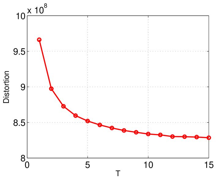
Figure 1: Distortion errors on the training set of SIFT1M vs different $T$(s) with $M=8$, $K=256$ and $C=2$.

5 Discussions

5.1 Connections

Our approaches are closely related with PQ [9] and CKM [24]. PQ splits the original vector into multiple subvectors to address the scalability issues. CKM rotates the space optimally and thus can achieve better accuracy. In each subspace, both PQ and CKM generate a single sub codebook and choose one sub codeword to quantize the original point. Our ECKM extends the idea by choosing multiple sub codewords from the single sub codebook, while our OCKM generates multiple sub codebooks, each of which contributes one sub codeword.

Next, we theoretically discuss the relations between our OCKM and others.

Theorem 1.

Under optimal solutions, we have:

$$f_{\text{ock},M,K,C}^{*} \leq f_{\text{ck},M,K}^{*}$$ (18)

$$f_{\text{ock},M,K,C}^{*} \leq f_{\text{eck},M,K,C}^{*}.$$ (19)

Proof.

If we limit $\mathbf{D}^{m,c_{1}}=\mathbf{D}^{m,c_{2}},c_{1},c_{2}\in\{1,\cdots,C\}$ in Eqn. 10, OCKM is reduced to the ECKM in Eqn. 6 by relations in Eqn. 8 and Eqn. 9, which proves the Eqn. 19.

Denote $\mathbf{R}_{\text{ck}},\{\mathbf{D}^{m}_{\text{ck}}\}_{m=1}^{M},\{\mathbf{b}_{i,\text{ck}}^{m}\}_{i=1,m=1}^{N,M}$ as the optimal solution of CKM in Eqn. 5. A feasible solution of OCKM can be constructed by

$$\mathbf{R}_{\text{ock}} =\mathbf{R}_{\text{ck}}$$

$$\mathbf{D}^{m,c}_{\text{ock}} =\begin{cases}\mathbf{D}_{\text{ck}}^{m}&c=1\\ \mathbf{0}&c\geq 2\end{cases}$$

$$\mathbf{b}_{i,\text{ock}}^{m,c} =\mathbf{b}_{i,\text{ck}}^{m}~{}~{}c\in\{1,\cdots,C\}.$$

With the constructed parameters, the objective function of OCKM remains the same with CKM, which proves the Eqn. 18. ∎

This theorem implies the proposed OCKM can potentially achieve a lower distortion error with the number of partitions $M$ and $K$ fixed.

Theorem 2.

Under the optimal solutions, we have,

$$f^{*}_{\text{ock},M^{\prime},K,C}\leq f_{\text{ck},M,K}^{*}$$ (20)

if $M^{\prime}=M/C$ and $M$ is divisible by $C$.

Proof.

The basic idea is for the optimal solution of CKM, every consecutive $C$ sub codebooks and the binary representation are grouped to construct a feasible solution of OCKM with an equal objective function.

Specifically, the construction is

$$\mathbf{R}_{\text{ock}} =\mathbf{R}_{\text{ck}}$$

$$\mathbf{D}_{\text{ock}}^{p,q} =\begin{bmatrix}\mathbf{0}_{(q-1)S\times K}\\ \mathbf{D}_{\text{ck}}^{(p-1)C+q}\\ \mathbf{0}_{(C-q)S\times K}\end{bmatrix}$$

$$\mathbf{b}_{i,\text{ock}}^{p,q} =\mathbf{b}_{i,\text{ck}}^{(p-1)C+q},$$

where $\mathbf{0}_{a\times b}$ is a matrix of size $a\times b$ with all entries being $0$, and $p\in\{1,\cdots,M^{\prime}\},q\in\{1,\cdots,C\}$. ∎

Take $C=2$, $M=2$ as an example. The formulation of CKM is

$$\min~{}~{} f_{\text{ck},2,K}=\sum_{i=1}^{N}\left\|\mathbf{x}_{i}-\mathbf{R}\begin{bmatrix}\mathbf{D}^{1}&\mathbf{0}\\ \mathbf{0}&\mathbf{D}^{2}\end{bmatrix}\begin{bmatrix}\mathbf{b}_{i}^{1}\\ \mathbf{b}_{i}^{2}\end{bmatrix}\right\|_{2}^{2}$$

$$\operatorname{s.t.}~{}~{} \mathbf{R}^{T}\mathbf{R}=\mathbf{I}$$

$$\mathbf{b}_{i}^{m}\in\{0,1\}^{K}$$

$$\|\mathbf{b}_{i}^{m}\|_{1}=1$$

Let $\mathbf{R}_{\text{ck}}$, $\{\mathbf{D}^{m}_{\text{ck}}\}_{m=1}^{2}$, $\{\mathbf{b}_{i,\text{ck}}^{m}\}_{i=1,m=1}^{N,2}$, be the optimal solutions of CKM. Then

$$\mathbf{R}_{\text{ock}} =\mathbf{\mathbf{R}}_{\text{ck}}$$

$$\mathbf{D}_{\text{ock}}^{1,1} =\begin{bmatrix}\mathbf{D}_{\text{ck}}^{1}\\ \mathbf{0}\end{bmatrix}$$

$$\mathbf{D}_{\text{ock}}^{1,2} =\begin{bmatrix}\mathbf{0}\\ \mathbf{D}_{\text{ck}}^{2}\end{bmatrix}$$

$$\mathbf{b}_{\text{ock}}^{1,c} =\mathbf{b}_{\text{ck}}^{c}~{}~{}c\in\{1,2\}$$

will be feasible for the problem of OCKM, i.e.

$$\min~{}~{} f_{\text{ock},1,K,2}=\sum_{i=1}^{N}{\left\|\mathbf{x}_{i}-\mathbf{R}\begin{bmatrix}\mathbf{D}^{1,1}&\mathbf{D}^{1,2}\end{bmatrix}\begin{bmatrix}\mathbf{b}_{i}^{1,1}\\ \mathbf{b}_{i}^{1,2}\end{bmatrix}\right\|_{2}^{2}}$$

$$\operatorname{s.t.}~{}~{} \mathbf{R}^{T}\mathbf{R}=\mathbf{I}$$

$$\mathbf{b}_{i}^{1,c}\in\{0,1\}^{K}$$

$$\|\mathbf{b}_{i}^{1,c}\|_{1}=1$$

and they have identical objective function values.

In Theorem 2, the code length of both approaches is $M/C\times C\times\log_{2}(K)=M\log_{2}(K)$, which ensures the distortion error of OCKM is not larger than that of CKM with the same code length.

Theorem 1 and Theorem 2 guarantee the advantages of our OCKM with multiple sub codebooks over the approach with single sub codebook.

5.2 Inequality Constraints or Equality Constraints

One may expect to replace the equality constraint $\|\mathbf{b}_{i}^{m,c}\|_{1}=1$ in Eqn. 10 as the inequality, i.e.

$$\|\mathbf{b}_{i}^{m,c}\|_{1}\leq 1.$$ (21)

This can potentially give a lower distortion under the same $M$ and $K$. However, under the same code length, this inequality constraint cannot be better than the equality constraints.

For the inequality case, there are $K+1$ different values for $\mathbf{b}_{i,\text{inequality}}^{m}$, i.e. $\|\mathbf{b}_{i,\text{inequality}}^{m,c}\|_{1}=0$, or $1$. The subscripts equality and inequality are used for the problem with the equality constraint and that with the inequality constraint, respectively. Then, the code length is $MC\log_{2}(K+1)$.

With the same code length, the equality case can consume $K+1$ sub codewords on each subvector. The size of $\mathbf{D}_{\text{equality}}^{m,c}$ is $S\times(K+1)$, and the size of $\mathbf{b}_{i,\text{equality}}^{m,c}$ is $(K+1)\times 1$.

From any feasible solution of the inequality case, we can derive the feasible solution of the equality case with the same objective function value, i.e.

$$\mathbf{R}_{\text{equality}} =\mathbf{R}_{\text{inequality}}$$

$$\mathbf{D}_{\text{equality}}^{m,c} =\begin{bmatrix}\mathbf{D}_{\text{inequality}}^{m,c},\mathbf{0}_{S\times 1}\end{bmatrix}$$

$$\mathbf{b}_{\text{equality}}^{m,c} =\begin{cases}\begin{bmatrix}\mathbf{b}_{\text{inequality}}^{m,c}\\ 0\end{bmatrix}&\text{if }\|\mathbf{b}_{\text{inequality}}^{m,c}\|_{1}=1\\ \begin{bmatrix}\mathbf{0}_{K\times 1}\\ 1\end{bmatrix}&\text{if }\|\mathbf{b}_{\text{inequality}}^{m,c}\|_{1}=0.\end{cases}$$

In the equality case, the last sub codeword is enforced to be $\mathbf{0}_{S\times 1}$, and the other sub codewords are filled by the one in the inequality case. If $\mathbf{b}^{m,c}_{\text{inequality}}$ is all $0$s, the entry of $\mathbf{b}_{\text{equality}}^{m,c}$ corresponding to the last sub codeword is set as $1$, or follows $\mathbf{b}^{m,c}_{\text{inequality}}$. This can ensure the multiplication $\mathbf{D}_{\text{equality}}^{m,c}\mathbf{b}_{\text{equality}}^{m,c}$ equals $\mathbf{D}_{\text{inequality}}^{m,c}\mathbf{b}_{\text{inequality}}^{m,c}$.

The objective function value remains the same, while with the optimal solution the equality case may obtain a lower distortion.

Algorithm 4 Optimization of OCKM

0:  $\{\mathbf{x}_{i}\}_{i=1}^{N}$, $M$

0:  $\mathbf{R}$, $\{\mathbf{D}^{m,c}\}_{m=1,c=1}^{M,C}$, and $\{\mathbf{b}_{i}^{m,c}\}_{i=1,m=1,c=1}^{N,M,C}$

1:  $\mathbf{R}=\mathbf{I}$

2:  Randomly initialize $\{\mathbf{D}^{m,c}\}_{m=1,c=1}^{M,C}$ from the data set.

3:  Update $\{\mathbf{b}_{i}^{m,c}\}_{i=1,m=1,c=1}^{N,M,C}$ by Alg. 2

4:  while !converged do

5:     Update $\mathbf{R}$

6:     Update $\{\mathbf{D}^{m,c}\}_{m=1,c=1}^{M,C}$

7:     for $i=1:N$ do

8:        for $m=1:M$ do

9:           Get ${\mathbf{new\_\hat{b}}}_{i}^{m,c}$ from Alg. 2

10:           if $g_{\text{ock}}({\mathbf{new\_\hat{b}}}_{i}^{m})<g_{\text{ock}}(\hat{\mathbf{b}}_{i}^{m})$ then

11:              $\hat{\mathbf{b}}_{i}^{m}={\mathbf{new\_\hat{b}}}_{i}^{m}$

12:           end if

13:        end for

14:     end for

15:  end while

5.3 Implementation

In OCKM and ECKM, there are three kinds of optimizers: rotation matrix $\mathbf{R}$, sub codebooks $\mathbf{D}^{m}$ or $\mathbf{D}^{m,c}$, and $\mathbf{b}_{i}^{m}$ or $\mathbf{b}_{i}^{m,c}$. In our implementation, $\mathbf{R}$ is initialized as the identity matrix $\mathbf{I}$. The sub codebook $\mathbf{D}^{m}$ and $\mathbf{D}^{m,c}$ are initialized by randomly choosing the data on the corresponding subvector.

The solution of $\mathbf{R}$, $\mathbf{D}^{m}$ and $\mathbf{D}^{m,c}$ are optimal in the iterative optimization process, but the solution of $\mathbf{b}_{i}^{m}$ and $\mathbf{b}_{i}^{m,c}$ are sub optimal. To guarantee that the objective function value is non-increasing in the iterative coordinate descent algorithm, we update $\mathbf{b}_{i}^{m}$ or $\mathbf{b}_{i}^{m,c}$ only if the codes of Alg. 1 or Alg. 2 can provide a lower distortion error. The whole algorithm of OCKM is shown in Alg. 4 and the one of ECKM can be similarly obtained.

The distortion errors of OCKM with different numbers of iterations are shown in Fig. 2 on SIFT1M (Sec. 6.1.1 for the dataset description), and we use $100$ iterations through all the experiments. The optimization scheme is fast and for instance on the training set of SIFT1M, the time cost of each iteration is about $4.2$ seconds in our implementations. (All the experiments are conducted on a server with an Intel Xeon 2.9GHz CPU.)

5.4 Distance Approximation for ANN search

In this subsection, we discuss the methods of the Euclidean ANN search by OCKM, and analyze the query time. Since ECKM is a special case of OCKM, we only discuss OCKM.

Let $\mathbf{q}\in\mathbb{R}^{D}$ be the query point. The approximate distance to $\mathbf{x}_{i}$ encoded as ${\hat{\mathbf{b}}_{i}}^{T}\triangleq\begin{bmatrix}{{}\hat{\mathbf{b}}_{i}^{1}}^{T}&\cdots&{{}\hat{\mathbf{b}}_{i}^{M}}^{T}\end{bmatrix}$ is

$$\text{distAD}(\mathbf{q},\hat{\mathbf{b}}_{i})$$ (22)

$$= \|\mathbf{q}-\mathbf{R}\hat{\mathbf{D}}\hat{\mathbf{b}}_{i}\|_{2}^{2}$$

$$= \|\mathbf{q}\|_{2}^{2}-2\sum_{m=1}^{M}\sum_{c=1}^{C}{{\mathbf{z}^{m}}^{T}(\mathbf{D}^{m,c}\mathbf{b}_{i}^{m,c})+\|\hat{\mathbf{D}}\hat{\mathbf{b}}_{i}\|_{2}^{2}}$$

$$\propto \frac{1}{2}\|\mathbf{q}\|_{2}^{2}-\sum_{m=1}^{M}\sum_{c=1}^{C}{{\mathbf{z}^{m}}^{T}(\mathbf{D}^{m,c}\mathbf{b}_{i}^{m,c})+\frac{1}{2}\|\hat{\mathbf{D}}\hat{\mathbf{b}}_{i}\|_{2}^{2}},$$ (23)

where $\mathbf{z}^{m}$ is the $m$-th subvector of $\mathbf{R}^{T}\mathbf{q}$.

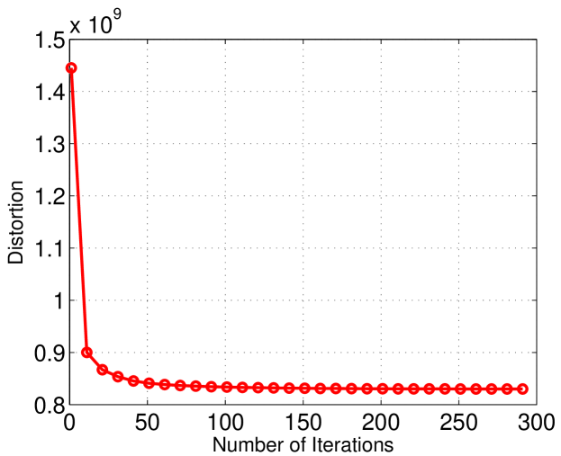
Figure 2: Distortion vs the number of iterations on the training set of SIFT1M with $M=8$, $K=256$ and $C=2$.

The first item $\|\mathbf{q}\|_{2}^{2}/2$ is constant with all the database points and can be ignored in comparison. The third item $\|\hat{\mathbf{D}}\hat{\mathbf{b}}_{i}\|_{2}^{2}/2$ is independent of the query point. Thus, it is precomputed once as the lookup table for all the quires. This precomputation cost is not low compared with the linear scan cost for a single query, but is negligible for a large amount of queries which is the case in real applications. Moreover, this term is computed only using the binary code $\hat{\mathbf{b}}_{i}$ and no access to the original $\mathbf{x}_{i}$ is required. For the second item, we can pre-compute $\{-{\mathbf{z}^{m}}^{T}\mathbf{d}_{k}^{m,c}\}_{k=1,m=1,c=1}^{K,M,C}$ and store it as the lookup tables. Then there are $MC+1$ table lookups and $MC+1$ addition operations to calculate the distance. The $1$ corresponds to the third item of Eqn. 23.

If the query point is also represented by the binary codes, denoted as $\hat{\mathbf{b}}_{q}$, we can recover $\mathbf{q}$ as $\mathbf{q}^{\prime}\triangleq\mathbf{R}\hat{\mathbf{D}}\hat{\mathbf{b}}_{q}$. Then the approximate distance to any database point will be identical with Eqn. 22, i.e.

$$\text{distSD}(\hat{\mathbf{b}}_{q},\hat{\mathbf{b}}_{i})=\text{distAD}(\mathbf{q}^{\prime},\hat{\mathbf{b}}_{i}).$$ (24)

Eqn. 22 is usually referred as the asymmetric distance while Eqn. 24 as the symmetric distance. Since the symmetric distance encodes both the query and the database points, the accuracy is generally lower than the asymmetric distance, which only encodes the database points.

Analysis of query time. We adopt an exhaustive search in which each database point is compared against the query point and the points with smallest approximate distances are returned. The exhaustive search scheme is fast in practice because each comparison only requires a few table lookups and additional operations.

Table II lists the code length and the comparison among PQ, CKM and our OCKM for exhaustive search. Under the same code length, OCKM consumes only one more table lookup and one more addition than the others. Considering the other computations in the querying, the differences of time cost are minor in practice.

Take $M_{\text{ck}}=8$, $K=256$, $C=2$, $M_{\text{ock}}=4$ as an example. The code length of OCKM and CKM are both $64$. The number of table lookups are $9$ for OCKM and $8$ for CKM. With these configurations on SIFT1M data set, the exhaustive querying over 1 million database points costs about $24.3$ms for OCKM and $23.5$ms for CKM in our implementations. Thus, the on-line query time is comparable with the state-of-the-art approaches, but the proposed approach can potentially provide a better accuracy.

TABLE II: Comparison in terms of the code length, the number of table lookups and the number of addition operations for exhaustive search.

	OCKM	CKM [24]	PQ [9]
Code Length	$MC\log_{2}(K)$	$M\log_{2}(K)$	$M\log_{2}(K)$
#(Table Lookups)	$MC+1$	$M$	$M$
#(Additions)	$MC+1$	$M$	$M$

6 Experiments

6.1 Settings

6.1.1 Datasets

Experiments are conducted on three widely-used high-dimensional datasets: SIFT1M [9], GIST1M [9], and SIFT1B [9]. Each dataset comprises of one training set (from which the parameters are learned), one query set, and one database (on which the search is performed). SIFT1M provides $10^{5}$ training points, $10^{4}$ query pints and $10^{6}$ database points with each point being a $128$-dimensional SIFT descriptor of local image structures around the feature points. GIST1M provides $5\times 10^{5}$ training points, $10^{3}$ query points and $10^{6}$ database points with each point being a $960$-dimensional GIST feature. SIFT1B is composed of $10^{8}$ training points, $10^{4}$ query points and as large as $10^{9}$ database points. Following [24], we use the first $10^{6}$ training points on the SIFT1B datasets. The whole training set is used on SIFT1M and GIST1M.

6.1.2 Criteria

ANN search is conducted to evaluate our proposed approaches, and three indicators are reported.

• Distortion: distortion is referred here as the sum of the squared loss after representing each point as the binary codes or the indices of the sub codewords. Generally speaking, the accuracy is better with a lower distortion.

• Recall: recall is the proportion over all the queries where the true nearest neighbor falls within the top ranked vectors by the approximate distance.

• Mean overall ratio: mean overall ratio  [34] reflects the general quality of all top ranked neighbors. Let $\mathbf{r}_{i}$ be the $i$-th nearest vector of a query $\mathbf{q}$ with the exact Euclidean distance, and $\mathbf{r}_{i}^{*}$ be the $i$-th point of the ranking list by the approximate distance. The rank-$i$ ratio, denoted by $R_{i}(\mathbf{q})$, is

  $$R_{i}(\mathbf{q})=\frac{\|\mathbf{q}-\mathbf{r}_{i}^{*}\|_{2}}{\|\mathbf{q}-\mathbf{r}_{i}\|_{2}}.$$

  The overall ratio is the mean of all $R_{i}(\mathbf{q})$, i.e.

  $$\frac{1}{k}\sum_{i=1}^{k}{R_{i}(\mathbf{q})}.$$

  The mean overall ratio is the mean of the overall ratios of all the queries. When the approximate results are the same as exact search results, the overall ratio will be $1$. The performance is better with a lower mean overall ratio.

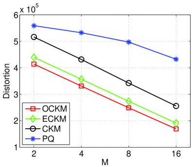
(a) SIFT1M	(b) GIST1M

Figure 3: Distortion on the training set.

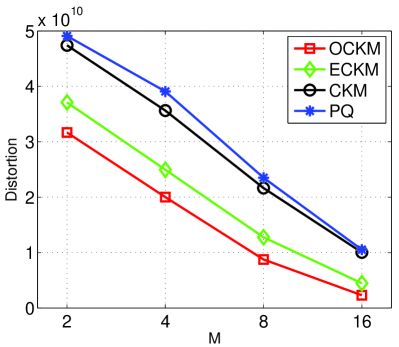
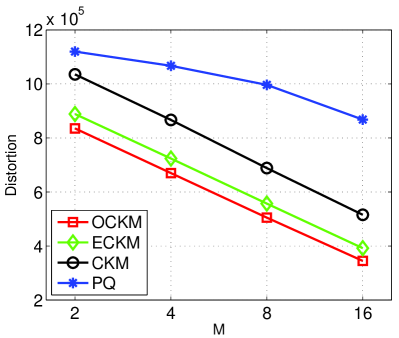
(a) SIFT1M	(b) GIST1M

Figure 4: Distortion on the database set.

6.1.3 Approaches

We compare our Optimized Cartesian $K$-Means (OCKM) with Product Quantization (PQ) [9] and Cartesian $K$-Means (CKM) [24]. Besides, the results of our extended Cartesian $K$-Means (ECKM) are also reported. Following [24], we set $K=256$ to make the lookup tables small and fit the sub index into one byte.

A suffix ‘-A’ or ‘-S’ is appended to the name of approaches to distinguish the asymmetric distance or the symmetric distance in ANN search. For example, OCKM-A represents the database points are encoded by OCKM, and the asymmetric distance is used to rank all the database points.

We do not compare with other state-of-the-art hashing algorithms, such as spectral hashing (SH) [40] and iterative quantization (ITQ) hashing [5], because it is demonstrated PQ is superior over SH [9] and CKM is better than ITQ [24].

6.2 Results

6.2.1 Comparison with the number of subvectors fixed

The distortion errors on the training set and database set are illustrated in Fig. 3 and Fig. 4, respectively. From the two figures, our OCKM achieves the lowest distortion, followed by ECKM. This is because under the same $M$, both CKM and ECKM are the special case of OCKM, as discussed in Theorem 1.

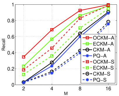
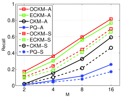
(a) SIFT1M	(b) GIST1M

Figure 5: Recall for ANN search at the $10$-th top ranked point.

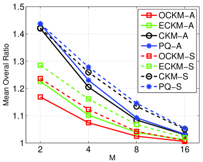
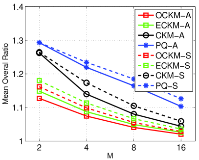
(a) SIFT1M	(b) GIST1M

Figure 6: Mean overall ratio for ANN search at the $10$-th top ranked point.

Fig. 5 and Fig. 6 show the recall and the mean overall ratio for ANN search at the $10$-th top ranked point, respectively. With the same type of the approximate distance, our approach OCKM achieves the best performance: the highest recall and the lowest mean overall ratio. With the lowest distortion errors demonstrated in Fig. 5 and Fig. 6, the OCKM is more accurate for encoding the data points.

32	64	128
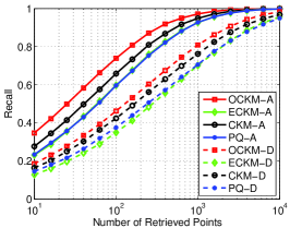
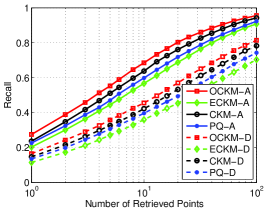
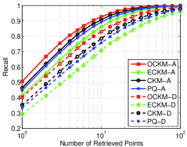
(a)	(b)	(c)
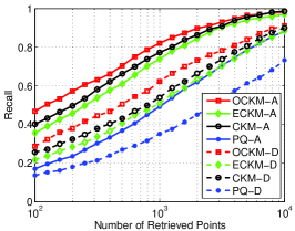
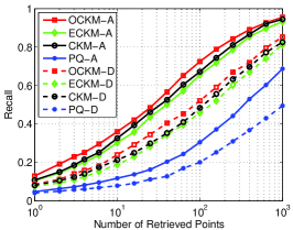
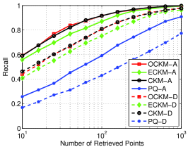
(d)	(e)	(f)
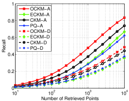
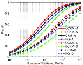
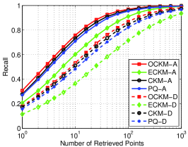
(g)	(h)	(i)

Figure 7: Recall for ANN search. The first row corresponds to SIFT1M; the second to GIST1M; and the third to SIFT1B. The code lengths are $32$, $64$ and $128$ from the left-most column to the right-most.

6.2.2 Comparison with the code length fixed

We use $M_{\text{ock}}$, $M_{\text{eck}}$, $M_{\text{ck}}$, $M_{\text{pq}}$ to denote the number of subvectors in OCKM, ECKM, CKM, and PQ, respectively. The code length of CKM is $M_{\text{ck}}\log_{2}(K)$, while the code length of OCKM is $M_{\text{ock}}C\log_{2}(K)$. Fixing $C=2$ as the analysis in Sec. 4.1.3, we set $M_{\text{ock}}=M_{\text{ck}}/2$ with $M_{\text{ck}}$ being $4$, $8$, and $16$ for code length $32$, $64$ and $128$, respectively. The $M_{\text{pq}}$ is identical with $M_{\text{ck}}$, while $M_{\text{eck}}$ is with $M_{\text{ock}}$. In this way, the code length is identical through all the approaches.

The results in terms of recall on SIFT1M, GIST1M, and SIFT1B are shown in Fig. 7. From these results, we can see that:

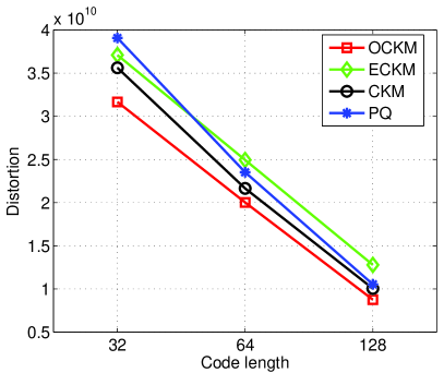
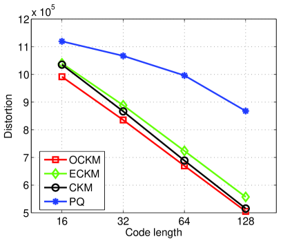
(a) SIFT1M	(b) GIST1M

Figure 8: Distortion under the same code length on the database set.

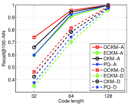
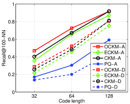
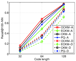
(a) SIFT1M	(b) GIST1M	(c) SIFT1B

Figure 9: Recall at the $100$-th top ranked point under the same code length.

• Generally, our OCKM outperforms all the others under the same type of approximate distance. For example of the asymmetric distance with 64 bits, the improvement of OCKM is about $5$ percents on SIFT1M in Fig. 7 (b), $4$ percents on GIST1M in Fig. 7 (e), $4$ percents on SIFT1B in Fig. 7 (h) at the $10$-th top ranked point. The performance of OCKM mainly benefits from the low distortion errors, which is also discussed in Theorem 2. Fig. 8 illustrates the distortion on the database under the same code length for SIFT1M and GIST1M. We can see under the same code length, our approach achieves the lowest distortions.

• The improvement is even better with a smaller code length. To present the observation more clearly, we extract the recall at the $100$-th nearest neighbor from Fig. 7 and plot Fig. 9. With a larger code length, the recalls of our OCKM and the second best CKM approach $1$. With a smaller code length, our OCKM gains larger improvement.

• ECKM is not quite competitive with the same code length. The possible reason is that the number of sub codebooks is smaller than those of the others. Take the code length of $64$ bits as an example. There are $8$ subvectors and each has one sub codebook for PQ and CKM, resulting in $8$ sub codebooks. OCKM is equipped with $4$ subvectors, but each has two sub codebooks, also resulting in $8$ sub codebooks. Comparatively, ECKM has $4$ subvectors, each of which has one sub codebook, and there are only $4$ sub codebooks in total. Smaller numbers of sub codebooks may degrade the performance of ECKM. Compared with SIFT1M and SIFT1B, ECKM achieves even better results than PQ on GIST1M, which indicates GIST1M is more sensitive to the rotation.

Fig. 10 illustrates the experiment results in terms of mean overall ratio with different code lengths on SIFT1M and GIST1M. Mean overall ratio captures the whole quality of the returned points while the recall captures the position of the nearest neighbor and ignores the quality of the other points. Under this criterion, our OCKM achieves the lowest mean overall ratio and outperforms all the others. This implies the returned nearest neighbors of OCKM are of high quality and close to the query points.

32	64	128

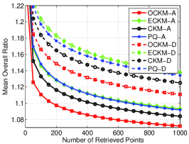
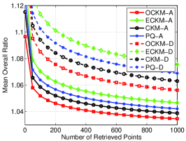
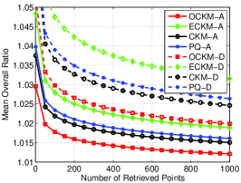
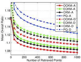
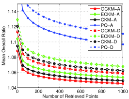
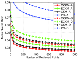
Figure 10: Mean overall ratio for ANN search. The results in the first row are on SIFT1M while those in the second row are on GIST1M. The first column corresponds to the code length $32$; the second to $64$; and the third to $128$.

7 Conclusion

In this paper, we proposed the Optimized Cartesian $K$-Means (OCKM) algorithm to encode the high-dimensional data points for approximate nearest neighbor search. The key idea of OCKM is that in each subspace multiple sub codebooks are generated and each sub codebook contributes one sub codeword for encoding the subvector. The benefit is that it reduces the quantization error with comparable query time under the same code length. The theoretical analysis and experimental results show that OCKM achieves superior performance for ANN search over state-of-the-art approaches.

Jianfeng Wang received his B.Eng. degree from the Department of Electronic Engineering and Information Science in the University of Science and Technology of China (USTC) in 2010. Currently, he is a PhD student in MOE-Microsoft Key Laboratory of Multimedia Computing and Communication, USTC. His research interests include multimedia retrieval, machine learning and its applications.

Jingdong Wang received the BSc and MSc degrees in Automation from Tsinghua University, Beijing, China, in 2001 and 2004, respectively, and the PhD degree in Computer Science from the Hong Kong University of Science and Technology, Hong Kong, in 2007. He is currently a Lead Researcher at the Visual Computing Group, Microsoft Research, Beijing, P.R. China. His areas of interest include computer vision, machine learning, and multimedia search. At present, he is mainly working on the Big Media project, including large-scale indexing and clustering, and Web image search and mining. He is an editorial board member of Multimedia Tools and Applications.

Jingkuan Song is currently a Research Fellow in University of Trento, Italy. He received his Ph.D degree from The University of Queensland, and BS degree in Software Engineering from University of Electronic Science and Technology of China. His research interest includes large-scale multimedia search, computer vision and machine learning.

Xin-Shun Xu received his M.S. and Ph.D. Degrees in computer science from Shandong University, China, in 2002, and Toyama University, Japan, in 2005, respectively. He joined the School of Computer Science and Technology at Shandong University as an associate professor in 2005, and joined the LAMDA group of the National Key Laboratory for Novel Software Technology, Nanjing University, China, as a postdoctoral fellow in 2009. Currently, he is a professor of the School of Computer Science and Technology at Shandong University, and the leader of MIMA (Machine Intelligence and Media Analysis) group of Shandong University. His research interests include machine learning, information retrieval, data mining, bioinformatics, and image/video analysis.

Heng Tao Shen is a Professor of Computer Science in School of Information Technology and Electrical Engineering, The University of Queensland. He obtained his B.Sc. (with 1st class Honours) and Ph.D. from Department of Computer Science, National University of Singapore in 2000 and 2004 respectively. He then joined the University of Queensland as a Lecturer and became a Professor in 2011. His research interests include Multimedia/Mobile/Web Search and Big Data Management. He is the winner of Chris Wallace Award for outstanding Research Contribution in 2010 from CORE Australasia. He is an Associate Editor of IEEE TKDE, and will serve as a PC Co-Chair for ACM Multimedia 2015.

Shipeng Li joined and helped to found Microsoft Research’s Beijing lab in May 1999. He is now a Principal Researcher and Research Area Manager coordinating multimedia research activities in the lab. His research interests include multimedia processing, analysis, coding, streaming, networking and communications. From Oct. 1996 to May 1999, Dr. Li was with Multimedia Technology Laboratory at Sarnoff Corporation as a Member of Technical Staff. Dr. Li has been actively involved in research and development in broad multimedia areas and international standards. He has authored and co-authored 6 books/book chapters and 280+ referred journal and conference papers. He holds 140+ granted US patents. Dr. Li received his B.S. and M.S. in Electrical Engineering (EE) from the University of Science and Technology of China (USTC), Hefei, China in 1988 and 1991, respectively. He received his Ph.D. in EE from Lehigh University, Bethlehem, PA, USA in 1996. He was a faculty member in Department of Electronic Engineering and Information Science at USTC in 1991-1992. Dr. Li received the Best Paper Award in IEEE Transaction on Circuits and Systems for Video Technology (2009). Dr. Li is a Fellow of IEEE.

References

- [1] S. Arya and D. M. Mount. Approximate nearest neighbor queries in fixed dimensions. In SODA, pages 271–280, 1993.
- [2] L. Cao, Z. Li, Y. Mu, and S.-F. Chang. Submodular video hashing: a unified framework towards video pooling and indexing. In ACM Multimedia, pages 299–308, 2012.
- [3] M. Datar, N. Immorlica, P. Indyk, and V. S. Mirrokni. Locality-sensitive hashing scheme based on p-stable distributions. In Symposium on Computational Geometry, pages 253–262, 2004.
- [4] J. H. Friedman, J. L. Bentley, and R. A. Finkel. An algorithm for finding best matches in logarithmic expected time. ACM Trans. Math. Softw., 3(3):209–226, 1977.
- [5] Y. Gong and S. Lazebnik. Iterative quantization: A procrustean approach to learning binary codes. In CVPR, pages 817–824, 2011.
- [6] J. He, J. Feng, X. Liu, T. Cheng, T.-H. Lin, H. Chung, and S.-F. Chang. Mobile product search with bag of hash bits and boundary reranking. In CVPR, pages 3005–3012, 2012.
- [7] J. He, W. Liu, and S. Chang. Scalable similarity search with optimized kernel hashing. In KDD, pages 1129–1138, 2010.
- [8] P. Indyk and R. Motwani. Approximate nearest neighbors: Towards removing the curse of dimensionality. In STOC, pages 604–613, 1998.
- [9] H. Jegou, M. Douze, and C. Schmid. Product quantization for nearest neighbor search. IEEE Trans. Pattern Anal. Mach. Intell., pages 117–128, 2011.
- [10] J. Ji, J. Li, S. Yan, B. Zhang, and Q. Tian. Super-bit locality-sensitive hashing. In NIPS, pages 108–116, 2012.
- [11] Y. Jia, J. Wang, G. Zeng, H. Zha, and X.-S. Hua. Optimizing kd-trees for scalable visual descriptor indexing. In CVPR, pages 3392–3399, 2010.
- [12] W. Kong and W.-J. Li. Isotropic hashing. In NIPS, pages 1655–1663, 2012.
- [13] B. Kulis and T. Darrell. Learning to hash with binary reconstructive embeddings. In NIPS, pages 1042–1050, 2009.
- [14] B. Kulis and K. Grauman. Kernelized locality-sensitive hashing. IEEE Trans. Pattern Anal. Mach. Intell., 34(6):1092–1104, 2012.
- [15] Y.-H. Kuo, K.-T. Chen, C.-H. Chiang, and W. H. Hsu. Query expansion for hash-based image object retrieval. In ACM Multimedia, pages 65–74, 2009.
- [16] W. Liu, J. Wang, R. Ji, Y. Jiang, and S. Chang. Supervised hashing with kernels. In CVPR, pages 2074–2081, 2012.
- [17] X. Liu, J. He, D. Liu, and B. Lang. Compact kernel hashing with multiple features. In ACM Multimedia, pages 881–884, 2012.
- [18] S. P. Lloyd. Least squares quantization in pcm. IEEE Transactions on Information Theory, 28(2):129–136, 1982.
- [19] J. B. MacQueen. Some methods for classification and analysis of multivariate observations. In Proceedings of the fifth Berkeley symposium on mathematical statistics and probability, volume 1, page 14, 1967.
- [20] S. Mallat and Z. Zhang. Matching pursuits with time-frequency dictionaries. IEEE Transactions on Signal Processing, pages 3397–3415, 1993.
- [21] Y. Mu and S. Yan. Non-metric locality-sensitive hashing. In AAAI, 2010.
- [22] M. Muja and D. G. Lowe. Fast approximate nearest neighbors with automatic algorithm configuration. In VISSAPP (1), pages 331–340, 2009.
- [23] M. Norouzi and D. Fleet. Minimal loss hashing for compact binary codes. In ICML, pages 353–360, 2011.
- [24] M. Norouzi and D. J. Fleet. Cartesian k-means. In CVPR, pages 3017–3024, 2013.
- [25] M. Raginsky and S. Lazebnik. Locality-sensitive binary codes from shift-invariant kernels. In NIPS, pages 1509–1517, 2009.
- [26] J. Revaud, M. Douze, C. Schmid, and H. Jegou. Event retrieval in large video collections with circulant temporal encoding. In CVPR, 2013.
- [27] R. Salakhutdinov and G. Hinton. Semantic hashing. Int. J. Approx. Reasoning, 50(7):969–978, 2009.
- [28] P. H. Schönemann. A generalized solution of the orthogonal procrustes problem. Psychometrika, 31(1):1–10, 1966.
- [29] G. Shakhnarovich, T. Darrell, and P. Indyk. Nearest-Neighbor Methods in Learning and Vision: Theory and Practice. The MIT press, 2006.
- [30] C. Silpa-Anan and R. Hartley. Optimised kd-trees for fast image descriptor matching. In CVPR, 2008.
- [31] J. Song, Y. Yang, Z. Huang, H. Shen, and R. Hong. Multiple feature hashing for real-time large scale near-duplicate video retrieval. In ACM Multimedia, pages 423–432, 2011.
- [32] J. Song, Y. Yang, Y. Yang, Z. Huang, and H. T. Shen. Inter-media hashing for large-scale retrieval from heterogeneous data sources. In SIGMOD, pages 785–796, 2013.
- [33] C. Strecha, A. Bronstein, M. Bronstein, and P. Fua. Ldahash: Improved matching with smaller descriptors. IEEE Trans. Pattern Anal. Mach. Intell., 34(1):66–78, 2012.
- [34] Y. Tao, K. Yi, C. Sheng, and P. Kalnis. Efficient and accurate nearest neighbor and closest pair search in high-dimensional space. ACM Trans. Database Syst., 35(3), 2010.
- [35] J. Wang and S. Li. Query-driven iterated neighborhood graph search for large scale indexing. In ACM Multimedia, pages 179–188, 2012.
- [36] J. Wang, J. Wang, N. Yu, and S. Li. Order preserving hashing for approximate nearest neighbor search. In ACM Multimedia, pages 133–142, 2013.
- [37] J. Wang, J. Wang, G. Zeng, R. Gan, S. Li, and B. Guo. Fast neighborhood graph search using cartesian concatenation. In ICCV, pages 2128–2135, 2013.
- [38] J. Wang, J. Wang, G. Zeng, R. Gan, S. Li, and B. Guo. Fast neighborhood graph search using cartesian concatenation. CoRR, abs/1312.3062, 2013.
- [39] J. Wang, N. Wang, Y. Jia, J. Li, G. Zeng, H. Zha, and X.-S. Hua. Trinary-projection trees for approximate nearest neighbor search. IEEE Trans. Pattern Anal. Mach. Intell., 36(2):388–403, 2014.
- [40] Y. Weiss, A. Torralba, and R. Fergus. Spectral hashing. In NIPS, pages 1753–1760, 2008.
- [41] H. Xu, J. Wang, Z. Li, G. Zeng, S. Li, and N. Yu. Complementary hashing for approximate nearest neighbor search. In ICCV, pages 1631–1638, 2011.
- [42] X. Zhu, Z. Huang, H. Cheng, J. Cui, and H. T. Shen. Sparse hashing for fast multimedia search. ACM Trans. Inf. Syst., 31(2):9, 2013.
- [43] X. Zhu, Z. Huang, H. T. Shen, and X. Zhao. Linear cross-modal hashing for effective multimedia search. In ACM Multimedia, 2013.