Properties and evolution of NEO families
created by tidal disruption at Earth

Abstract

We have calculated the coherence and detectable lifetimes of synthetic near-Earth object (NEO) families created by catastrophic disruption of a progenitor as it suffers a very close Earth approach. The closest or slowest approaches yield the most violent ‘s-class’ disruption events where the largest remaining fragment after disruption and reaccumulation retains less than 50% of the parent’s mass. The resulting fragments have a ‘string of pearls’ configuration after their reaccummulation into gravitationally bound components (Richardson et al., 1998). We found that the average absolute magnitude ($H$) difference between the parent body and the largest fragment is $\Delta H\sim 1.0$. The average slope of the absolute magnitude ($H$) distribution, $N(H)\propto 10^{(0.55\pm 0.04)\,H}$, for the fragments in the s-class families is steeper than the slope of the NEO population (Mainzer et al., 2011) in the same size range. The families remain coherent as statistically significant clusters of orbits within the NEO population for an average of $\bar{\tau}_{c}=(14.7\pm 0.6)\times 10^{3}$ years after disruption. The detectable lifetimes of tidally disrupted families are extremely short compared to the multi-Myr and -Gyr lifetimes of main belt families due to the chaotic dynamical environment in NEO space — they are detectable with the techniques developed by Fu et al. (2005) and Schunová et al. (2012) for an average duration ($\bar{\tau}_{det}$) ranging from about 2,000 to about 12,000 years for progenitors in the absolute magnitude ($H_{p}$) range from 20 to 13 corresponding to diameters in the range from about 0.5 to 10$\,\mathrm{km}$ respectively. The maximum absolute magnitude of a progenitor capable of producing an observable NEO family (i.e. detectable by our family finding technique) is $H_{p,max}=20$ (about $350\,\mathrm{m}$ diameter). The short detectability lifetime explains why zero NEO families have been discovered to-date. Nonetheless, every tidal disruption event of a progenitor with diameter greater than $0.5\,\mathrm{km}$ is capable of producing several million fragments in the $1\,\mathrm{m}$ to $10\,\mathrm{m}$ diameter range that can contribute to temporary local density enhancements of small NEOs in Earth’s vicinity. We expect that there are about 1,200 objects in the steady state NEO population in this size range due to tidal disruption assuming that one $1\,\mathrm{km}$ diameter NEO tidally disrupts at Earth every 2,500 years. These objects may be suitable targets for asteroid retrieval missions due to their Earth-like orbits with corresponding low $v_{\infty}$ which permits low-cost missions. The fragments from the tidal disruptions evolve into orbits that bring them into collision with terrestrial planets or the Sun or they may be ejected from the solar system on hyperbolic orbits due to deep planetary encounters. The end-state for the fragments from a tidal disruption at Earth have $\sim 5\times$ the collision probability with Earth compared to the background NEO population.

Key Words: NEAR-EARTH OBJECTS, ASTEROIDS, DYNAMICS, ASTEROIDS, COMPOSITION

1 Introduction

In this work we evaluate some of the physical and observable properties of tidally disrupted NEO families including their dynamical evolution and coherence time scales, and their observable lifetimes with modern asteroid surveys. Our eventual aim is to set a limit on the production rate of tidally disrupted NEO families for comparison with theoretical expectations.

When an asteroid makes a close approach to within about the Roche limit of a planet it may suffer morphological modifications due to tidal forces depending on the circumstances of the encounter and the asteroid’s physical construction. Inside the Roche limit a self-gravitating synchronously rotating liquid satellite orbiting a spherical planet has no stable equilibrium (Roche, 1849; Chandrasekhar, 1969) The structural changes may be as modest as lifting layers of surface material (e.g. Nesvorný et al., 2010), or as violent as splitting the asteroid into a binary (e.g. Walsh & Richardson, 2008) or tearing it completely apart in the manner of comet Shoemaker-Levy-9 (e.g. Asphaug et al., 1996). The tidal disruption of a progenitor by a terrestrial planet is one of the most likely creation scenarios for NEO families due to the relatively high close encounter probability of the NEOs with those planets (Fu et al., 2005), however, there are as-yet no statistically robust dynamical NEO families (Schunová et al., 2012).

Our claim that there are no known NEO families purposefully ignores the well-known dynamical association between some meteor showers and their cometary or asteroidal sources because they do not correspond to the traditional usage of the ‘family’ term that implies an orbital relationship between much larger objects. Similarly, it has been suggested that the Apollo asteroid (3200) Phaethon, the widely recognized progenitor of the Geminid meteoroid stream (e.g. Whipple, 1983; Jewitt & Li, 2010), is dynamically related to several other NEOs such as 2005 UD (Ohtsuka et al., 2006; Jewitt & Hsieh, 2006) and 1999 YC (Ohtsuka et al., 2008). This set of asteroids is thought to be the remnant of a comet disintegration. The connection between Phaethon and 2005 UD in particular was proposed as a result of the similarity of their orbits, their past dynamical evolution, and the fact that both are optically blue which is uncommon for NEOs. But the dynamical association was not confirmed in the rigorous statistical analysis of Schunová et al. (2012) — the orbital similarity between the two objects is not statistically significant.

Despite the lack of evidence for tidally disrupted NEO families in the observed NEO population the existence of double craters on the surfaces of Venus, Earth and Mars (Melosh & Stansberry, 1991), multiple crater chains (known as ‘catenae’) on the Moon and other natural satellites (Melosh & Whitaker, 1994), and the bizarre shapes of some NEOs as revealed by delay-Doppler radar images (e.g. Ostro et al., 1995; Bottke et al., 1999b) imply that close encounters and tidal disruption events are common in the NEO population since binaries and multiple systems, a ‘string of pearls’ fragment distribution, and strange shapes, are all expected outcomes of the tidal disruption process (e.g. Richardson et al., 2002).

The different morphologies of the tidal disruptions are in part due to the NEOs being relatively fragile ‘rubble-pile’ asteroids composed of the jumbled and re-accumulated remains of the aftermath of many previous disruptions (e.g. Richardson et al., 1998; Pravec & Harris, 2000). Further evidence of the rubble-pile structure of asteroids is the sharp limit in their spin period distribution at $P\sim 2.2$ hours for asteroids with $H<22$ (larger than about $200\,\mathrm{m}$ diameter). The period corresponding to the rotation barrier agrees well with the theoretical rotation rate limit for objects with a density of $\sim$2.7 g cm^-3 (Harris, 1996; Pravec & Harris, 2000). Asteroids that spin faster than the observed limit experience a centrifugal acceleration on the surface that exceeds the local gravitational acceleration leading to mass loss through spalling or complete rotational disruption of the object.

In situ evidence for the asteroids’s rubble pile constitution come from spacecraft missions to the NEOs (243) Mathilde and (25143) Itokawa by the NEAR (e.g. Yeomans et al., 1997) and Hayabusa spacecraft (e.g. Fujiwara et al., 2006) respectively which revealed that their inner structure must be porous. Direct imaging from the spacecraft revealed obvious rubble pile structures on their surfaces, with loosely distributed boulders and gravel, and crater morphologies that can only be explained if they are due to impacts on a weak or fragmented target (e.g. Greenberg et al., 1994; Love & Ahrens, 1996). Perhaps conclusively, Asphaug et al. (1996) showed that the tidal disruption of comet Shoemaker-Levy-9 (SL9) by Jupiter matches the observed disruption event if the progenitor had a rubble pile construction.

Mild tidal events might be also capable of producing meteoroid streams. The close passage of an object by a planet can lift material from the surface that then spreads along the object’s orbit with time due to the small $\Delta v$ imparted by the lifting process and gravitational perturbations by other objects in the solar system (Kornoš et al., 2009; Tóth et al., 2011). After hundreds of years the particles will be distributed along the entire orbit and will produce meteors and fireballs if they enter Earth’s atmosphere. However, due to the single-event nature of the tidal disruption the stream would not be replenished and the putative meteoroid stream could only be observed for a short time after creation. Tóth et al. (2011) calculated the maximum activity of a meteor shower originating from the putative Pribram meteorite progenitor to be only 1 meteor in 8 days visible from a single observing place.

Richardson et al. (1998) performed numerical simulations of NEO distortion and disruption by Earth’s tides using more realistic asteroid shapes, spin rates, axis orientations, perigee distance $q$, relative speed at infinity $v_{\infty}$ and body orientation at periapse, and identified four classes of tidal encounter outcomes (that should not be confused with the capital letters used to identify asteroid taxonomic classes):

s)

catastrophic disruptions in which the largest remaining fragment retains less than 50% of the parent’s mass (similar to SL9),

b)

rotational breakup in which the largest remaining fragment retains 50%-90% of the parent’s mass,

m)

mild disruption in which less than 10% of the parent’s original mass is lost and,

n)

no mass loss but possible morphological modification.

They found that the result of the disruption is primarily determined by the relative speed at infinity $v_{\infty}$ and periapse distance $q$. The most violent s-class disruptions occur at small periapse distances at low speeds because this configuration allows the objects to spend more time in Earth’s proximity and consequently offers more time for the tidal forces to act on the body. In a simplified case of an NEO rapidly rotating in the prograde direction (i.e. when the angle between the object’s rotational pole and the north ecliptic pole is $<90\arcdeg$), centrifugal acceleration and tidal forces act together to cause mass shedding and/or disruption so that the range of $q$ and $v_{\infty}$ where the disruptions occur widens as the rotation rate increases. On the other hand, retrograde rotation reduces the severity of disruption and mass loss and may even prevent the disruption (Richardson et al., 1998).

While the state of tidal disruption modeling is mature and continues to improve both in theory and in the lab, comparatively little has been done on estimating the rate at which disruptions actually take place and understanding the evolution of the fragments after the disruption process. An NEO with $D>1\,\mathrm{km}$ ($H_{p}\lesssim 17.5$) suffers an s-class event near Earth or Venus roughly every 3,200 years and some kind of disruption event (M-, B- and s-class) occurs once about every 1,000 years (Richardson et al., 1998). More recently Tóth et al. (2011) calculated that the frequency of tidal disruptions of any kind for NEOs with $D>200\,\mathrm{m}$ ($H_{p}\lesssim 21$) is $\sim 1.6\times 10^{-4}$/year or roughly one tidal disruption every 6,200 years — within a factor of 2 of the Richardson et al. (1998) disruption rate. Our eventual goal is to measure or set a limit on the disruption rate in an effort to distinguish between the two calculations and thereby test the entire NEO orbit and disruption modeling process.

If the disruption rate is high enough, and the fragments remain dynamically distinguishable as a tidally disrupted family long enough, then it should be possible to identify them in the NEO population. However, recent attempts to identify families in the NEO population all yielded zero candidates (e.g. Drummond, 2000; Fu et al., 2005; Schunová et al., 2012). While several NEO clusters were identified they could not be shown to be statistically significant. The main goals of this work are to determine the coherence and detectable lifetimes of tidally disrupted NEO families and use this information to set an observational limit on the number of tidally disrupted NEO families.

The tidal disruption of an NEO could pose an increased impact threat to Earth above and beyond that calculated from the current NEO models (e.g. Bottke et al., 1994, 2002; Ivanov, 2008) that do not account for local enhancements in the orbit element phase space due to families. Since asteroids tend to repeat their trajectories and encounters, if an asteroid is tidally disrupted at Earth then it is likely that the fragments will also return to Earth’s environs. A limit on the frequency of disruption events that lead to the creation of NEO families will thus provide the necessary information to assess their effect on the NEO collision rate with Earth.

2 Method

We carried out $N$-body simulations of the tidal disruptions of roughly spherical gravitationally-bound ‘rubble-pile’ asteroids on a range of Earth-crossing orbits and their subsequent gravitational reaccumulation into secondary objects. The secondaries form a tidally disrupted NEO family that we integrate forward in time for $10^{7}\,\mathrm{yr}$ to inspect their orbital evolution, and applied a cluster identification algorithm (Schunová et al., 2012) at logarithmically time-spaced intervals to measure the families’ coherence time (i.e. the time during which they can be detected as a cluster of objects on similar orbits). We then employed the Pan-STARRS1 Moving Object Processing System (Denneau et al., 2013) to simulate observational selection effects and calculated the NEO families’ detectable lifetimes. Finally, we measured the families’ size-frequency distribution and the porosity of the family members.

2.1 Simulating tidal disruptions at Earth

We used the method developed by Granvik et al. (2012) and implemented in the OpenOrb software package (Granvik, 2009) to generate 10,000 NEOs on Earth encountering orbits with flat distributions in all six orbit elements with semi-major axes in the range $0.5\,\mathrm{AU}<a<7.4\,\mathrm{AU}$, eccentricities with $0<e<1$, inclinations ($i$) from $0^{\circ}$ to $90^{\circ}$, and angular elements spanning $[0\arcdeg,360\arcdeg)$. In this way our results can be easily normalized to match any desired NEO model. Initial epochs for the tidal-disruption simulations were randomly chosen within one synodic lunar period (29.530589 days) starting on MJD 55461 (2010 Sep 22). The randomization over all possible geometries between the earth, Moon and Sun would require extending the initial epoch distribution over the 19-year Metonic Cycle but we assumed that our choice will have a negligible effect on our results because the dynamics of NEOs are dominated by close planetary encounters on time scales that are much longer than the Metonic cycle or synodic lunar period. We then down-selected the NEOs to the 718 objects with $v_{\infty}\leq 35\,\mathrm{km}\,\mathrm{s}^{-1}$ and $q\leq 2.5\,R_{\earth}$, the limiting values enveloping tidal disruption events near Earth (Richardson et al., 1998), and performed N-body simulations of their passage through the Earth-Moon system.

The synthetic NEOs are rubble pile models consisting of about 2,000 solely gravitationally-bound identical rigid $120\,\mathrm{m}$ diameter ‘unit’ spheres. Thus, the smallest possible fragment in our simulations is a single unit sphere with absolute magnitude $H_{0}=22.2$ assuming a geometric albedo of $\rho=0.15$. The unit spheres were arranged in Hexagonal Closest Packing (HCP, Leinhardt et al., 2000) to form roughly spherical progenitors with diameters of $\sim 2\,\mathrm{km}$. However, to a large extent, the tidal disruption process is independent of the dimensions of the unit spheres and the progenitor (Solem & Hills, 1996) and we are free to scale the unit spheres as needed to simulate both larger and smaller objects.

The simulations assigned every unit sphere a density of $\rho=3,340\,\mathrm{kg}\,\mathrm{m}^{-3}$ and yielded progenitors with a bulk density of $\sim 2,130\,\mathrm{kg}\,\mathrm{m}^{-3}$ and porosity $\Phi_{p}\sim 37$% at the realized average packing efficiency of $\sim 63$%. These values are in good agreement with measurements of rubble-pile NEOs with similar dimensions such as (25143) Itokawa (Abe et al., 2006), the binary (66391) 1999 KW₄ (Ostro et al., 2006), and the triple NEO 1994 CC (Brozović et al., 2011).

While the size of a synthetic progenitor is not particularly important in the disruption simulation its shape and rotation period are critical. Oblate and prolate objects are more easily disrupted than spherical ones and faster rotation periods also enhance the tidal disruption process. The complete parameter space determining tidal disruption outcome was examined in earlier works (e.g. Richardson et al., 1998; Walsh & Richardson, 2006) but we want to set an upper limit on the tidal disruption rate while at the same time not wasting CPU time. We balanced these objectives by using roughly spherical progenitors generated with the HCP technique but using a median spin rate of $P=4.3\,\mathrm{h}$ (Pravec et al., 2002) for NEOs with H$<$22 and a disruption-favorable prograde spin-axis. The overall effect should be to enhance the tidal disruption rate of our progenitors above the actual rate such that we can set an upper limit.

Every simulation was set in the planetocentric frame with 50,000 time steps of 5 seconds each corresponding to roughly 3 days for modeling the entire disruption process. The starting distance was 20 Earth radii from Earth, so the fragments typically traveled roughly 40 Roche radii ($\sim$ 100 Earth radii) during the simulation time and by the end of the simulation they were far away enough from Earth that tidal forces were negligible. From that time in the simulation we numerically integrated the particles under the forces of all the planets in the solar system (see §2.3 below).

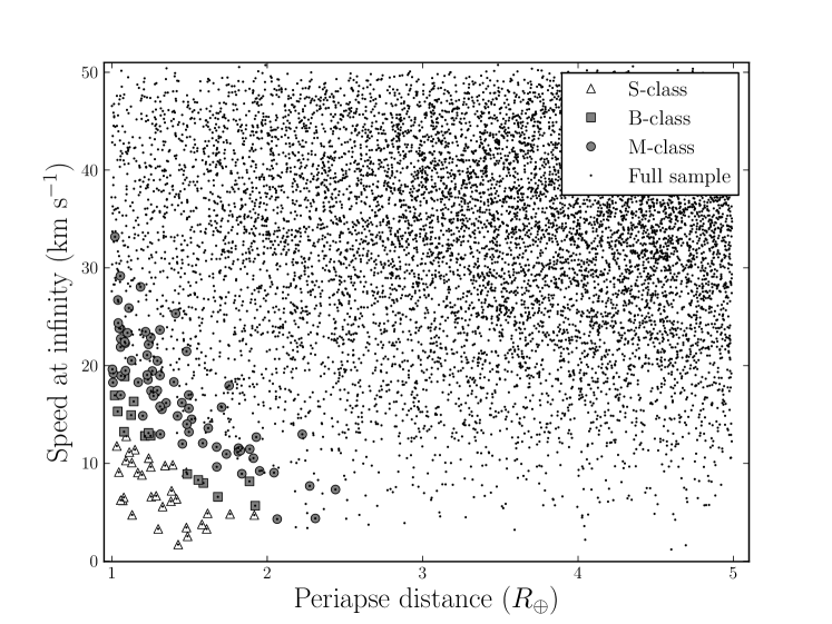
Figure 1: Speed at infinity ($v_{\infty}$) vs. minimum geocentric distance (periapse, $q$) for 10,000 synthetic tidal disruption progenitors.

Fig. 1 illustrates that the 120 disrupted objects all have $v_{\infty}\lesssim 35.0\,\mathrm{km}\,\mathrm{s}^{-1}$ and $q\lesssim 2.5\,R_{\earth}$ and it is evident that the disruptions become more violent as each parameter decreases (i.e. the progenitor suffers more loss of material). The most violent s-class disruptions take place exclusively when the object approaches Earth within $2\,R_{\earth}$, less than half the distance to geostationary orbit, and at speeds $\leq 15\,\mathrm{km}\,\mathrm{s}^{-1}$, consistent with the results of Richardson et al. (1998) and Walsh & Richardson (2006) (as expected since we used their software for our simulations).

A total of 120 of the 718 tidal disruption simulations produced more than two fragments — the rest were either gentle events with no disruption or binary-producing events. We ignored the binaries because it has already been established that identifying genetically linked NEO pairs in a statistically significant manner is exceedingly difficult (Schunová et al., 2012). As expected, the majority (73) of the disruptions were of the mild m-class, while roughly half as many progenitors (32) suffered the deep encounters required for s-class disruption. In the remainder of this paper we usually consider only the 32 s-class disruptions.

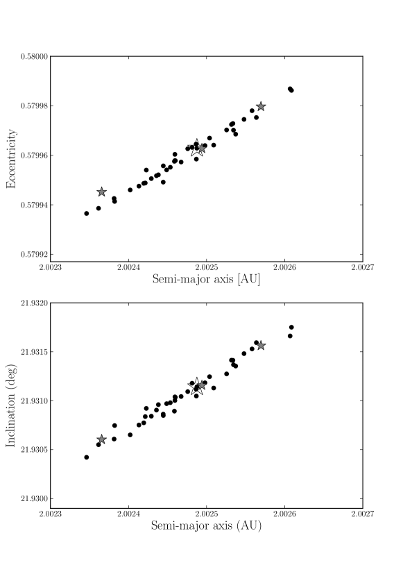
Figure 2: Post-disruption configuration of members of a synthetic NEO family created in a s-class tidal disruption. (top) eccentricity vs. semi-major axis and (bottom) inclination vs. semi-major axis. The large white star represents the position of the largest fragment and the filled gray stars represent the positions of the next three largest members of the family. ‘Post-disruption’ means the end of the pkdgrav tidal disruption simulation when we begin our n-body integration of all the fragments under the influence of all major bodies in the solar system. The simulations typically end when the fragments are beyond $\sim 100{R}_{\earth}$.

The $\sim 27$% of our simulations that generated s-class tidal disruptions created what we call s-class families in which the progenitor is shattered and the fragments are configured in a ‘string of pearls’ tidal stream (see Fig. 2). The members of the family have very similar orbital elements and a power-law size-frequency distribution (SFD) where the mass is distributed along the string rather then concentrated at its center. We think that s-class families will eventually be detected in the NEO population and this work determines their dynamical and detectable lifetime.

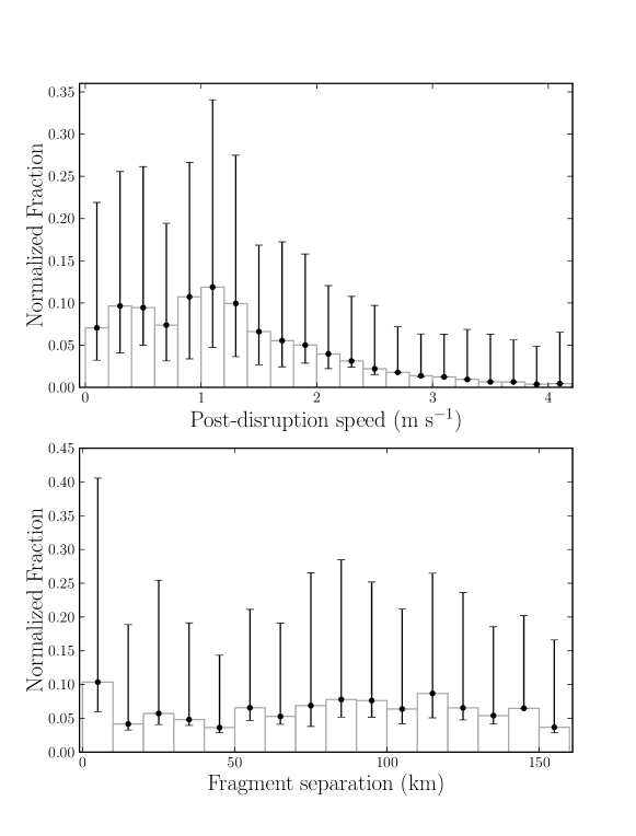
Figure 3: Post-disruption speed and separation of members of synthetic s-class NEO families created by tidal disruption near Earth when the fragments are well beyond Earth’s Roche limit at the end of the n-body disruption simulation (typically beyond $\sim 100{R}_{\earth}$). Both values are always with respect to the largest remnant in each family. The error bars represent the asymmetric RMS variation of the fractional distribution in the bin across all the synthetic s-class families.

The maximum post-disruption speed ($v_{pd}$) of $\sim 4\,\mathrm{m}\,\mathrm{s}^{-1}$ (see Fig. 3) is much less than speeds typical of impact-generated catastrophic disruptions in the main belt that can reach up to half the impact speed of the projectile (the typical impact speed in the main belt is $\sim 5\,\mathrm{km}\,\mathrm{s}^{-1}$, Bottke et al. (e.g. 2001); Scheeres et al. (e.g. 2002)). The average post-disruption speed of s-class family members is $v_{pd}\sim 1.2\,\mathrm{m}\,\mathrm{s}^{-1}$ — less than the escape speed for a $2\,\mathrm{km}$ rubble pile asteroid. The average speed is about $10\times$ higher than predicted by Tóth et al. (2011) who calculated that the speed of boulders escaping the surface of a rubble pile NEO during close Earth encounters is $\gg\sim 1\,\mathrm{m}\,\mathrm{s}^{-1}$.

It is interesting that the fragments can escape even though their relative velocities with respect to the largest fragment at tidal disruption were less than the escape speed (see Fig. 3). They can do so because tidal disruptions are gentle events during which tidal effects continue to gently accelerate the fragments away from each other well after the primary disruption event. In the case of NEO tidal disruptions at Earth the initial disruption generates an average of about $0.4\,\mathrm{m}\,\mathrm{s}^{-1}$ relative speed between the fragments that increases asymptotically almost another 50% to about $0.6\,\mathrm{m}\,\mathrm{s}^{-1}$ at the end of the simulation. By the end of the simulation the fragments are no longer gravitationally bound because there are several tens to hundreds of kilometers separation between them and it is appropriate to continue the simulations with a long-term dynamical orbit integrator (see §2.3).

2.2 NEO tidal disruptions at other terrestrial planets

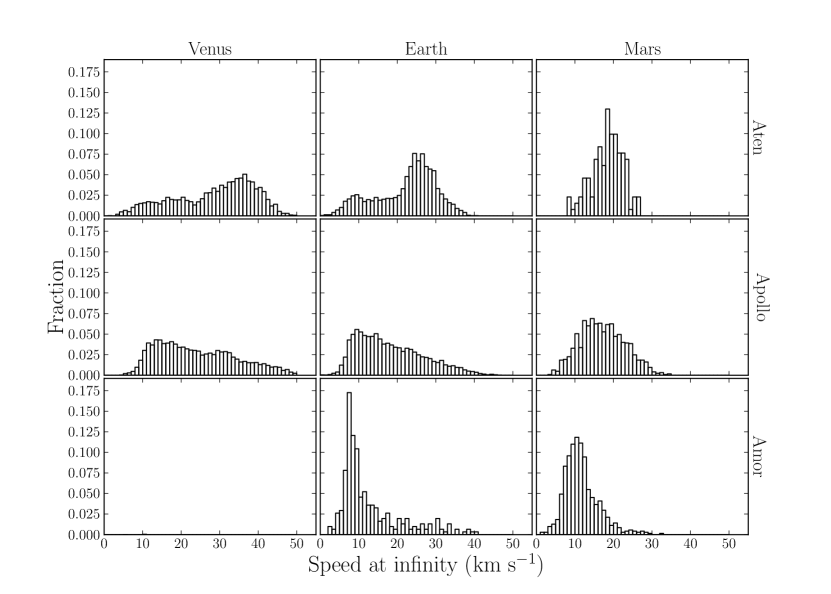
Figure 4: Distributions of the relative $v_{\infty}$ for Amor, Apollo and Aten groups at Venus, Earth and Mars. Amor asteroids never approach Venus (lower left panel) but their velocity distributions with Mars and Earth peak at small values favorable to tidal disruption.

We excluded all the other terrestrial planets and the Moon from consideration because they are not expected to contribute a significant flux of tidally disrupted families in NEO phase space. This is mostly due to the distribution of $v_{\infty}$ for the NEO dynamical sub-groups at the planets as illustrated in Fig. 4.

Mercury is relatively easy to exclude as a source of s-class NEO families because of 1) its small mass 2) the low spatial density of NEOs that can approach it and 3) their high encounter speeds.

Venus and Earth have almost $10\times$ larger collision probabilities with NEOs than Mercury and Mars (Bottke et al., 1994). We estimate that Venus is about 1/3 as effective as Earth at producing s-class disruption families because 1) about 42% of NEOs are on Venus-crossing trajectories compared to $\sim 84$% on Earth-crossing orbits (Bottke et al., 2002) and 2), since NEOs are typically moving faster near Venus than when approaching Earth, only about 56% of them have $v_{\infty}<30\,\mathrm{km}\,\,\mathrm{s}^{-1}$ with respect to Venus while $\sim 86$% of the Earth-crossing NEOs have slow enough approach speeds to allow effective tidal disuption (see Fig. 4). Thus, Venus contributes to the tidally disrupted NEO family population at about 33% the rate contributed by Earth.

It is possible that Mercury and Venus could disrupt ‘rogue’ asteroids that are not NEOs (${\it e.g.}$ objects on orbits that are entirely interior to Earth’s orbit (e.g.  Zavodny et al., 2008) that could make a close passage by either Mercury or Venus and the fragments could then evolve into NEO phase space) but this possibility is small and, in any event, we will show below that the detectable lifetime of tidally disrupted NEO families is short. Thus, it is unlikely that tidally disrupted families created in this manner will stay coherent and evolve into NEO space in a time frame that will allow them to be detectable.

The Moon was excluded because its smaller Roche sphere makes it much less efficient than Earth at disrupting rubble piles (Richardson et al., 1998) (the ratio of the cross-sectional area of the Moon’s Roche sphere to Earth’s is only $\sim 0.074$).

Finally, despite Mars being only 1/10^th Earth’s mass it 1) is much closer to the Main Belt, 2) orbits the Sun in a region with a much higher flux of asteroids and 3) NEO encounter speeds are slower than at Earth which would yield an increased tidal disruption probability — so it is not immediately obvious whether it will create more or less s-class NEO families than Earth. The mean impact rate of $1\,\mathrm{km}$ diameter NEOs on Mars is predicted to be about $10\times$ smaller than the impact rate of the same-size NEOs on Earth (Bottke et al., 1994) and, since the impact rate on Earth is about one $1\,\mathrm{km}$ diameter NEO every $\sim 6\times 10^{5}$ years (e.g. Stuart, 2003), the rate on Mars is about once every $\sim 6\times 10^{6}$ years. The interval between close encounters with Mars sufficient for s-class disruption roughly scales as the cross-sectional area of its Roche sphere compared to the planet, so that the s-class disuption rate is still on the Myr time scale.

To estimate the number of NEO families created near Mars by tidal disruption it is also necessary to account for the Intermediate source Mars-crossers (IMC) that feed the NEO population (Bottke et al., 2002). The IMCs are to Mars as NEOs are to Earth — they are the subset of the Mars-crossing asteroid population that borders the main belt with orbital parameters $q>1.3\,\mathrm{AU}$, $2.06\,\mathrm{AU}\leq a\leq 2.48\,\mathrm{AU}$ or $2.52\,\mathrm{AU}\leq a<2.8\,\mathrm{AU}$, with $i\lesssim 15^{\circ}$, and a combination of ($a$,$e$,$i$) values such that they cross the orbit of Mars during a secular oscillation cycle of their eccentricity (Bottke et al., 2002; Migliorini et al., 1998). Michel et al. (2000) estimates that there are about $4\times 10^{4}$ IMCs with $D>1$ km with an average lifetime of $\tau_{MC}\sim 29$ Myr and, during their lifetime, about 4% of IMCs suffer encounters within 3 Mars radii of Mars — about 1 close approach every $\sim 18,000$ years. Our Mars tidal disruption simulations suggest that there is $\sim$17% probability of a close Mars encounter resulting in a s-class tidal disruption so we estimate that there is one family created by tidal disruption every 100,000 years. Since this time is considerably longer than the predicted disruption rates at Earth (e.g. Richardson et al., 1998; Tóth et al., 2011), and because the most likely s-class disruptions at Mars are of IMCs, not NEOs, we exclude Mars-induced tidal disruptions in the NEO population from consideration.

2.3 Post-disruption dynamical integrations

The geocentric position and velocity of the tidal disruption fragments at the last time step (MJD=55499) were converted back to their heliocentric values and numerically integrated forward in time for 60 Myr. All the integrations used the N-body Burlisch-Stoer algorithm from the Mercury6 software package (Chambers, 1999) with variable time steps that allows good tracking of the orbital evolution during close encounters with planets. The initial timestep was set to 3 days.

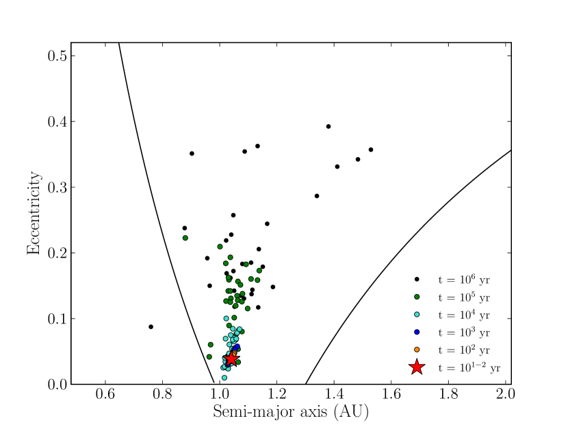
Figure 5: Time evolution of eccentricity and semi-major axis of the members of a single s-class NEO tidal disruption. This family is detectable for 70,000 years using the method described in §2.5.

The orbital time evolution of the members of a s-class family as illustrated in Fig. 5 proceeds rapidly as expected for an object in the inner solar system on a planet-crossing orbit. The progenitor has an orbit with perihelion near Earth and the orbits of the fragments remain practically unchanged during the first few hundred years in which individual fragments become evenly distributed along the original orbit (i.e. throughout the whole range of mean anomaly) forming a possible meteoroid stream (e.g. Tóth et al., 2011). In this particular family the members then evolve to higher eccentricity over the next 10s of thousands of year and only then begin to spread in semi-major axis. All the fragments remained as NEOs throughout the first $10^{6}\,\mathrm{yr}$.

We included only gravitational forces in our integrations because NEOs of the size of our smallest fragments with $H=23$ ($D\sim 100\,\mathrm{m}$) are influenced by non-gravitational forces on timescales much longer than the coherence time scale of the tidally disrupted NEO families. The most recently measured average Yarkovsky drift rate for km-scale NEOs with albedos measured by WISE is $\sim 10^{-9}\,\mathrm{AU}$/year (Nugent et al., 2012) with the rate being a few times higher for $100\,\mathrm{m}$-scale objects. Our measured average ‘dynamical drift rate’ for the tidally disrupted fragments in our simulations was about $1,000\times$ higher i.e. the average rate of evolution of the fragments just under the gravitational influence of the major objects in the solar system. Since the non-gravitational effects are minimal even on the smallest objects in our simulation we are justified in ignoring their effect on all the objects.

2.4 Simulating observational selection effects

We need to account for selection effects in the detection of the fragments to assess the ability to detect NEO families created through catastrophic tidal disruption. Observational selection effects will favor brighter objects at any ($a$,$e$,$i$) values and surveys will preferentially discover those objects on low-inclination orbits for which the objects approach Earth closely and slowly (e.g. Jedicke et al., 2003). The latter effect favors the detection of tidal disruption fragments because objects on those types of orbits are precisely those that are most likely to be disrupted. The former effect makes tidally disrupted NEO families more difficult to detect because a small but detectable progenitor will disrupt into smaller fragments for which not enough members are detectable by modern surveys.

We simulated observational selection effects representative of the entire known NEO population using the Pan-STARRS Moving Object Processing System (MOPS, Denneau et al., 2013) and the full sample of 250,000 NEOs from the Synthetic Solar System Model (S3M) (Grav et al., 2011). We used the 47 lunation survey configuration of (Granvik et al., 2009) because they showed that it is a good proxy for all surveys that have discovered NEOs to-date and roughly reproduces the number of known NEOs and their orbit distribution. The fact that the simulation does so implies that it can roughly simulate the observational selection effects imprinted on the known NEO population and on the synthetic members of tidally disrupted NEO families in our study.

The PS1 survey and the NEO simulation are described in detail in the last three references but, briefly, the Pan-STARRS1 system (Kaiser et al., 2010) has a $7\,\mathrm{deg}^{2}$ field of view and is able to reach a limiting magnitude of $V_{lim}\sim 21.7$ with their $w_{\rm P1}$ filter. To mimic the known NEO population the NEO simulation used a limiting magnitude of $V_{lim}\sim 22.7$ (following Granvik et al. (2009)) and included both opposition fields and small solar elongation fields (morning and evening ‘sweet spots’;  Chesley & Spahr, 2004)) covering a region of up to $5,500\,\mathrm{deg}^{2}$ per lunation. Each field is visited twice on three different nights within a lunation with a minimum of four days between the visits. To mimic weather, 25% of the nights are randomly excluded. When an object is bright enough to be detected MOPS links detections on the same night into ‘tracklets’. This is followed by inter-night linking of the tracklets into ‘tracks’ that are then tested for consistency with detections of an object on a heliocentric orbit. Objects with tracklets on at least three nights spread over the course of 7-10 days will yield a good orbit determination with Pan-STARRS1’s astrometric accuracy of about $0.1\arcsec$ (Milani et al., 2012).

We ran the orbits for all 1720 fragments from the 32 s-class tidal disruptions at 10 different epochs (0, 1, 10, 100, 10k, 20k, 50k, and 100k years after disruption) through the 47 lunation MOPS simulation to determine their detectability. We used a fixed $H=0$ for all the fragments simply to determine if and when the objects appeared in the simulated survey and their apparent $V$ magnitudes at those times. i.e. fragment $i$ has apparent magnitude $V_{i}(t,0)$ at time $t$ with $H=0$. We could then assign any absolute magnitude $H_{i}$ to a fragment and determine its apparent magnitude in the MOPS simulation as $V_{i}(t,H_{i})=V_{i}(t,0)+H_{i}$ (e.g. Harris, 1998). This allowed us the flexibility of assigning any SFD to the families including varying the size of the progenitor, the size of the largest fragment, and the slope of the distribution. Once the apparent magnitude was calculated for each fragment in each field we then determined whether it was above the simulated Pan-STARRS1 limiting magnitude ($V_{lim}\sim 22.7$) to determine if the fragment was detected. There had to be at least two detections of the same (moving) object per night to form a tracklet and multiple tracklets of the same object over several nights were required for the orbit determination. We did not account for trailing losses in the detection algorithm because the losses are relatively small for the typical rates of motion of the fragments in the survey ($<1\,\mathrm{deg}$/day).

The quality of orbit determination is crucial for assessing the statistical significance of NEO clusters (Schunová et al., 2012). Thus, in this work we applied stricter criteria for NEO detection than the actual Pan-STARRS1 survey for which the first NEO detections are complemented by follow-up observations at other observatories. We required that the arc length (in time) for an NEO family member be $\geq 90$ days and that the object be detected with $\geq 3$ tracklets in at least one lunation with additional tracklets in other lunations. With these requirements in place the orbital uncertainties are reduced to the level that makes it viable to search for NEO clusters in the known population comparable to the family search of Schunová et al. (2012).

2.5 Identifying NEO families

We adopted the cluster identification method developed by Fu et al. (2005) that we used previously to search for families in the known NEO population (Schunová et al., 2012). The method relies on identifying tight clustering of family members’ orbit elements using the Southworth & Hawkins (1963) orbital similarity criterion ($D_{SH}$) that incorporates all 5 Keplerian orbital elements.

The cluster identification method is described in detail by Schunová et al. (2012) and Fu et al. (2005) but we provide a short primer here. The technique recognizes that when families form and evolve in orbit element space the entire family may fit within the ‘envelope’ of the cluster but individual members may form a set of tightly linked pairs spanning a sub-set of the envelope. As time passes the envelope increases in size, the pairs become more widely spaced and the links between them are ‘broken’ as the density of the members in orbit element space decreases. The envelope of fragments is identified as a cluster in the 5-dimensional orbit element space because they all have mutual $D_{SH}<D_{cluster}$ (the $D_{SH}$ cluster threshold). The tightly linked sub-set is identified as the set of member pairs with mutual $D_{SH}<D_{pair}$ where $D_{pair}<D_{cluster}$. The largest set of paired fragments that all have $D_{SH}<D_{pair}$ is called the ‘string’ (because they are all connected with $D_{SH}<D_{pair}$). Finally, every candidate NEO cluster must fulfill two conditions:

• String size to cluster size ratio $SCR>SCR_{min}$

• Pair fraction $PF>PF_{min}$

where the string and cluster sizes are the number of objects in the string and cluster respectively and the pair fraction is the actual number of identified pairs divided by the total number of possible pairs in the cluster.

In our earlier work we showed that $D_{cluster}=0.06$, $D_{pair}=0.05$, $SCR_{min}=0.75$ and $PF_{min}=0.5$ allowed statistically significant identification of clusters of objects with $>4$ members (Schunová et al., 2012). One 4 member cluster was identified in the NEO population but only at the 2- to 3-$\sigma$ significance level.

3 Results

3.1 Orbit distribution of precursor bodies to tidally-disrupted NEO families

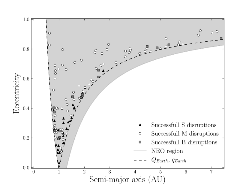
Figure 6: Eccentricity vs. semi-major axis of NEO progenitors that underwent M, B and s-class disruptions. The NEO region is depicted by the shaded area. The left and right dashed lines that converge at $a\sim 1$ AU correspond to orbits having aphelion and perihelion at Earth’s perihelion and aphelion distance respectively.

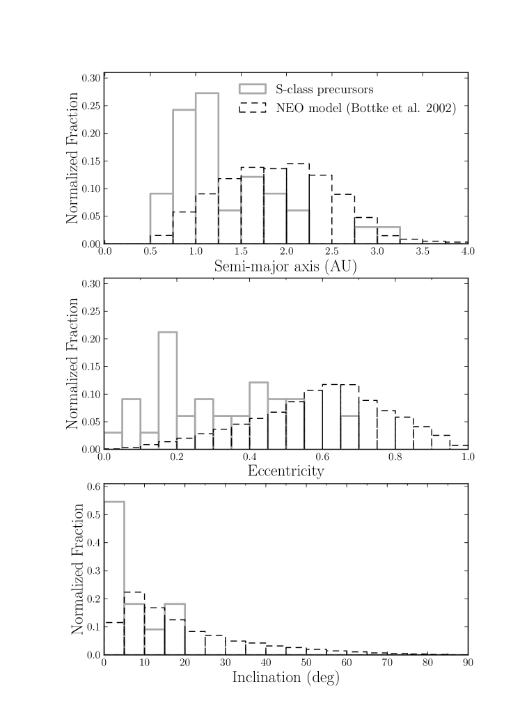
Figure 7: Fractional distribution of semi-major axis, eccentricity and inclination for NEOs from the Bottke et al. (2002) NEO model (dashed) and NEO progenitors (solid grey) that result in s-class tidal disruptions by Earth.

Pre-encounter orbits that result in tidal disruptions usually have aphelion or perihelion distances that lie near Earth’s orbit and the s-class disruptions of interest in this work are more tightly clustered along the Earth aphelion and perihelion lines than the M- and b-class disruptions (Fig. 6). More generally, the s-class disruption probability is enhanced for objects on orbits with $0.5\,\mathrm{AU}<a<1.25\,\mathrm{AU}$, $e<0.5$ and $i<5^{\circ}$ (Fig. 7) so that the progenitors’ orbit distribution is a subset of the entire NEO population (Bottke et al., 2002). This is a result of the fact that these types of orbits are more tangential to Earth’s orbit and the objects therefore spend more time in Earth’s environs where they may be subject to disruption. Note that more than half of all the s-class disruptions occur in the $i<5^{\circ}$ bin. This is interesting because it is now generally thought that the Bottke et al. (2002) NEO model under-represents the fraction of the population on these low-inclination orbits by about a factor of 2 in the sub-km size range (Mainzer et al., 2011). Thus, there may be more NEOs on orbits subject to s-class disruptions than this figure suggests.

A possible explanation for the enhancement of low-inclination NEOs (e.g. Mainzer et al., 2011; Rabinowitz et al., 1993; Greenstreet et al., 2012) is that it is because of a recent tidal disruption event that has increased the population of objects on Earth-like orbits in the NEO population. The enhanced number of objects in Earth-like orbits will increase the Earth-impact rate above current estimates and would increase the likelihood of the Earth capturing temporary satellites (Granvik et al., 2012).

3.2 Porosity & size-frequency distribution
of tidally disrupted NEOs

The size-frequency distribution (SFD) of the fragments in a tidally disrupted NEO family is critical to the determination of its detectability. Schunová et al. (2012)’s NEO family detection method requires that $>4$ known members be brighter than a limiting absolute magnitude $H_{max}=23$. In our simple model the number of objects in the family brighter than the limit depends on 3 factors: the absolute magnitude of the progenitor ($H_{p}$), the difference between the absolute magnitudes of the largest fragment and the progenitor ($\Delta H_{1}$), and the slope $\alpha$ of the SFD. The cumulative SFD for the fragments is then

$$N(H)=10^{\alpha(H-H_{1})}=10^{\alpha(H-H_{p}-\Delta H_{1})}$$ (1)

i.e. there are $N(H^{\prime})$ fragments with $H<H^{\prime}$ in the family with the largest fragment having an absolute magnitude of $H_{1}=H_{p}+\Delta H_{1}$. We used the results of our s-class tidal disruption simulations to determine the values of $\Delta H_{1}$ and $\alpha$.

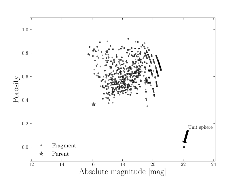
Figure 8: Porosity of s-class disruption fragments as a function of the absolute magnitude of the fragment. Some fragments have absolute magnitudes brighter than the progenitor, and most fragments have a higher porosity, due to a ‘fluffy’ re-accumulation/re-arrangement of the unit spheres after disruption. The points that lie along discretized curves near $H_{frag}\sim 20$ are due to fragments built from a small number of unit spheres. Fragments consisting of only one unit sphere have $\Phi=0$ as shown in the lower right.

To calculate a fragment’s absolute magnitude we assumed that it is spherical, has an albedo of 0.15, and radius as provided by pkdgrav. This will overestimate the absolute magnitude because pkdgrav provides the dimension of the fragment’s longest axis as the ‘radius’. For example, a ‘fragment’ consisting of two unit spheres has a ‘radius’ equal to twice the unit sphere radius. The problem is illustrated in Fig. 8 which shows that the porosity ($\Phi$) of the fragments is always higher than the porosity of the progenitor (by porosity we mean the macro-porosity — the fraction of the volume of an object occupied by voids). The discretized $\Phi$ values near $H_{frag}\sim 20$ are due to fragments that are built from a small number of unit spheres.

The tidal disruption process first increases the porosity of the progenitor as its equipotential surface is stretched towards Earth while approaching perigee before disruption into an s-class family. The disruption fragments continue to evolve and re-accumulate while still under the influence of tidal tension thereby ‘fluffing’ the internal structure of the larger fragments by increasing the size of internal void spaces. The resulting high-porosity elongated fragments might resemble the NEO (1620) Geographos (e.g. Bottke et al., 1999a; Walsh & Richardson, 2006) but these elongated and loosely bound rubble pile fragments probably cannot survive long in this state. Moderate-scale collisions or another series of close encounters together with self-gravity will decrease the macro-porosity by gradually collapsing the void spaces.

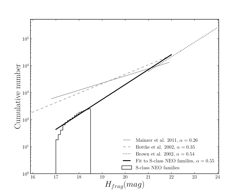
Figure 9: Three measured cumulative NEO SFDs for the real population (Mainzer et al. 2011, Bottke et al. 2002, Brown et al. 2002) and the SFD of our synthetic s-class disruption fragments with a fit as described in §3.2.

The determination of the s-class family SFD slope ($\alpha$) from the tidal disruption simulations was also problematic due to the discretization of the unit spheres and the relatively small number of fragments in each disruption. To overcome the latter problem we combined all our s-class disruption fragments. Even then, we could only fit the resulting SFD over a narrow range of absolute magnitudes from the largest fragment ($H_{1}$) to $H^{*}$, the absolute magnitude where the porosity (and mass and size) of the fragments becomes discretized, because of a clear turnover in the SFD caused by the unit sphere discretization. We empirically determined $H^{*}$ by starting with just the two largest family members and iteratively adding more members as we monitored the slope of the SFD. $H^{*}$ was fixed at the value where the SFD began to decrease, $H^{*}=18.5$, at which the fragment diameter is $\sim 6\times$ that of a unit sphere. This technique results in a cumulative SFD with a slope of $\alpha=0.55\pm 0.04\mathrm{(stat.)}$ (see Fig. 9).

Given that the calculated absolute magnitude of the fragments is problematic, we estimated the systematic uncertainty in the slope by recalculating each fragment’s absolute magnitude in a ‘worst case’ scenario assuming that the fragments have the same porosity as the progenitor instead of using pkdgrav’s diameter. The average change in absolute magnitude for the fragments was about $+0.7$ mags i.e. the fragments became smaller and their absolute magnitudes increased. This technique yielded a slope of $\alpha=0.66$ so we took the systematic uncertainty on the slope to be $\mathcal{O}(0.11)$.

Our measured slope of $\alpha=0.55\pm 0.04\mathrm{(stat.)}\pm 0.11\mathrm{(sys.)}$ is steeper than the SFDs of the overall NEO population of $\alpha=0.35\pm 0.02$ (for $H<22.0$;  Bottke et al., 2002) and from WISE observations where $\alpha=0.26\pm 0.03$ (for $H>17$;  Mainzer et al., 2011). On the other hand, our results are consistent with the slope of $0.54\pm 0.02$ measured from fireballs (Brown et al., 2002) in the size range from $1\,\mathrm{cm}$ to $200\,\mathrm{m}$ ($21\lesssim H\lesssim 43$) and with the SFD of $\alpha\sim 0.56$ for surface boulders on the NEO (25143) Itokawa in the 20 cm to $20\,\mathrm{m}$ size range (corresponding to $26\lesssim H\lesssim 36$;  Saito et al., 2006). Furthermore, the measured slopes are in agreement with the theoretical value of $0.5$ for self-similar collisional systems (e.g. Dohnanyi, 1969; O’Brien & Greenberg, 2005). The steep slope for the s-class families is also consistent with the suggestion of Tóth et al. (2011) that the tidal disruption of rubble-pile asteroids may increase the SFD slope of the NEO population.

We do not consider the absolute magnitude (or porosity) ‘problem’ to be serious for four reasons. First, while some of the fragments have outrageously high porosities of $>90$% the bulk of them lie in the 40-60% range compatible with measured values for NEOs and main belt asteroids. For example, (25143) Itokawa has a porosity of about 40% (Fujiwara et al., 2006) while Baer et al. (2011) showed that porosities of main belt asteroids smaller than 300 km in diameter range from 40% to 60% or more with the highest measured asteroid porosity being 75%. Second, and as discussed in the last paragraph, our measured SFD slope is consistent with the slope of small NEOs, expectations for fragments from tidal disruptions, and the theoretical value for self-similar collision cascades. Third, in our analysis below (§3.4) we will use 0.5 mag bins in the progenitors’s absolute magnitude — on the scale of the worst case error in the calculated absolute magnitudes. Thus, we will use a value of $\alpha=0.55\pm 0.11$ recognizing that the uncertainty is dominated by the systematic errors in our analysis. Finally, we note that the spin-frequency distribution (Warner et al., 2009) of all asteroids shows a well-known discontinuity at about $100\,\mathrm{m}$ that suggests a transition from a rubble pile internal structure to monoliths at about that diameter — thus, it is possible that there really is an actual discretization of asteroid interiors with a fundamental building block size of $\sim 100\,\mathrm{m}$.

3.3 Dynamical lifetime and coherence time of tidally disrupted s-class NEO families

Several dynamical mechanisms operating in the NEO region are capable of significantly increasing the orbital eccentricities and inclinations of NEOs that eventually cause them to impact the Sun, a planet, or be ejected from the solar system (Gladman et al., 2000). NEOs can also evolve onto hyperbolic orbits or suffer collisions with terrestrial planets. We will compare the end states of NEOs created in s-class tidal disruptions at the Earth to the overall NEO population in §3.5 but we measured their average dynamical lifetime to be $\sim 10$ Myr in agreement with Gladman et al. (2000) i.e. the time at which half of the tidally disrupted NEOs remain in the NEO population. The dynamical lifetime of the families sets an upper limit to the families’ coherence time.

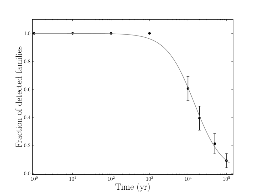
Figure 10: The fraction $f$ of the 32 s-class NEO families created by tidal disruption during a close encounter of their progenitors with Earth that are detectable as families as a function of time. The data was fit to a function of the form $f(t)=\{1+\exp[(\log_{10}(t)-\log_{10}(\tau_{c}))/w_{c}]\}^{-1}$ yielding a coherence time of $\tau_{c}=(14.7\pm 0.6)\times 10^{3}\,\mathrm{yr}$ when 50% of the families can be detected.

We define the coherence time for an NEO family to be the time duration during which the family members can be identified using our cluster identification algorithm described in §2.5 without taking into account the fragments’ detectability by astronomical surveys i.e. when the cluster identification is based solely on the similarity of the members’ orbital elements. To measure the coherence time we extracted the orbits of each member of each family from the numerical integration at 10 epochs: at $t=0\,\mathrm{yr}$, $t=10^{k}\,\mathrm{yr}$ with $k=0-6$, and at 20 and 50 kyr. Then we applied our cluster identification algorithm to each family at each epoch. All the s-class families can be identified as clusters for only the first 1,000 years (Fig. 10) and the average coherence time of the 32 families is $(14.7\pm 0.6)\times 10^{3}\,\mathrm{yr}$ (i.e. the average time after disruption for which $\geq 50$% of the families remain dynamically coherent). This time scale is extremely rapid compared to most of the known main belt families with ages of $>10^{6}\,\mathrm{yr}$ or even the youngest family associated with (1270) Datura that has an age of $\sim(450\pm 50)\times 10^{3}\,\mathrm{yr}$ (Nesvorny et al., 2006).

The coherence time depends on the parameters of the cluster finding algorithm which, in turn, were selected on their ability to discriminate NEO clusters within the background NEO orbit element population (Schunová et al., 2012). An alternative cluster finding algorithm may thus yield longer (or shorter) coherence times. For instance, the Earth’s atmosphere acts as a ‘cluster finding algorithm’ in the sense that it can be used to identify meteoroid streams that intersect Earth’s orbit in the form of meteor showers. The typical meteoroid stream coherence time of roughly 1,000 years (e.g. Tóth et al., 2011) is $\sim 10\times$ shorter than our measured value for tidally disrupted NEO familes because the concept of the NEO family changes from meteoric dust size particles to asteroid-sized particles, and because meteor streams are strongly influenced by non-gravitational forces like the Yarkovsky effect and radiation pressure.

3.4 Detectable lifetime of tidally disrupted NEOs

The coherence time sets an upper limit on the clusters’ detectable lifetime — the time during which the family members may be discovered by current surveys — because the coherence time does not account for observational selection effects as described in §2.4. Observational limitations will reduce the time during which a family can be identified because some of its members will not be detected due to their unfavorable observing geometry, rate of motion, or faintness. If there are not enough ($>4$) family members above the limiting absolute magnitude the family itself is simply undetectable using the Schunová et al. (2012) technique. Thus, we define the ‘detectability lifetime’ ($\tau_{det}$) as the time during which members of tidally disrupted NEO families can be efficiently discovered by ground-based asteroid surveys and identified as a statistically significant cluster in orbit element space.

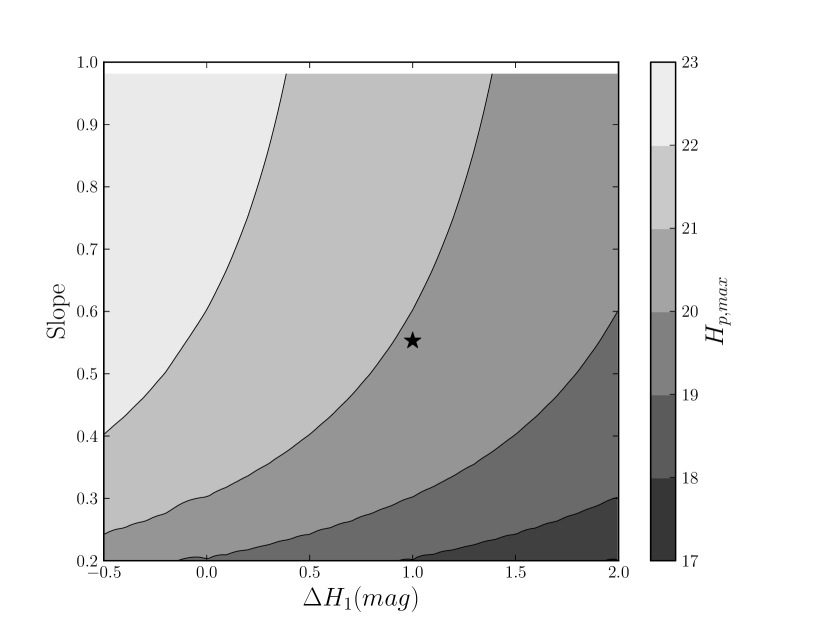
Figure 11: Maximum absolute magnitude ($H_{p,max}$) of a tidal disruption progenitor able to produce a detectable NEO family as a function of the fragments’ size-frequency distribution slope ($\alpha$) and the difference between the absolute magnitudes of the progenitor and the largest fragment ($\Delta H_{1}$). The star near the center represents our measured values from the pkdgrav simulations of s-class disruptions (see §3.2).

The smallest detectable progenitor’s diameter (see Fig. 11) must increase 1) as the difference in size between the progenitor and largest fragment increases and 2) as the SFD slope decreases. Both results are as expected because smaller fragments are more difficult to detect, and a shallow SFD produces only a few large fragments above the limiting absolute magnitude (i.e. there might not be enough of them to be detected as a statistically significant cluster with our method). While Fig. 11 spans the full range of slopes and $\Delta H_{1}$ from our tidal disruption simulations (§3.2), the smallest detectable progenitor’s diameter (maximum absolute magnitude, $H_{p,max}$) of an ‘average’ tidally disrupted s-class family has $H_{p,max}\sim 20$ (for $\bar{\alpha}\sim 0.55$ and $\mkern 1.5mu\overline{\mkern-1.5mu\Delta H_{1}\mkern-1.5mu}\mkern 1.5mu\sim 1.0$). This absolute magnitude corresponds to minimum progenitor diameters of $\sim 0.3\,\mathrm{km}$ and $\sim 0.77\,\mathrm{km}$ assuming albedos of 0.2 and 0.03 typical of S- and C-class asteroids respectively (Mainzer et al., 2011).

We applied our cluster detection algorithm on the family members detected in the survey simulation (§2.4) as we did to calculate the coherence time (§3.3). The fragments were assigned absolute magnitudes according to the average SFD with $\Delta H_{1}=$1 mag and $\alpha=0.55$. We then measured the detectable lifetime of all the families as a function of the progenitors’ absolute magnitude in 0.5 magnitude $H$ steps (Fig. 12) for two cases: 1) all detectable objects of any absolute magnitude and 2) where the detected fragments must have $H<23$ for consistency with the null result found in our earlier work (Schunová et al., 2012).

The detectability lifetime decreases as expected as the size of the progenitor decreases — smaller progenitors produce even smaller fragments that are difficult to detect. The measured value decreases smoothly from about 11,500 years at $H_{p}=13$ (about 10 km diameter) to about 5,000 years at $H_{p}=18$ (about 1 km diameter). The detectable lifetime then drops precipitously for families produced by the smallest progenitors, those with $H_{p}=20$ that are just barely capable of producing a detectable family, such that families produced by progenitors with $H_{p}=19.5$ can only be identified with our technique for $\sim 2,000$ years. This is simply because the smallest progenitors do not produce enough large fragments to remain above the survey systems’ limiting magnitude.

The probability of actually identifying tidally disrupted NEO families depends on the relative rates of their production and their lifetime ($L$ or $\tau$) such that the number of detectable families in the steady state population at any time is $N=FL$ where $F$ is the production ’flux’ rate. Since the observed number is $N=0$ (Schunová et al., 2012) a limit can be placed on the flux rate as described in §4.2.

3.5 End states of tidal disruption fragments

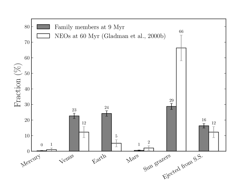
Figure 13: (shaded) End-states of fragments from tidal disruption of NEOs at Earth after 9 Myr compared to (white) the dynamical NEO population from Gladman et al. (2000) after 60 Myr. The average fraction is provided above the error bar for each bin.

About 9 Myr after the s-class tidal disruption at Earth about 50% of all the fragments are no longer NEOs because they have struck Earth, Venus or the Sun, or were ejected from the solar system (Fig. 13). Roughly one-quarter of all the fragments strike either Earth or Venus while the Sun attracts a slightly higher percentage (though nearly identical to within our statistics). The fraction of fragments that strike the Sun is smaller than the fraction of the generic NEO population simply because there is a smaller fraction available left to do so after about half of them have already struck Earth and Venus.

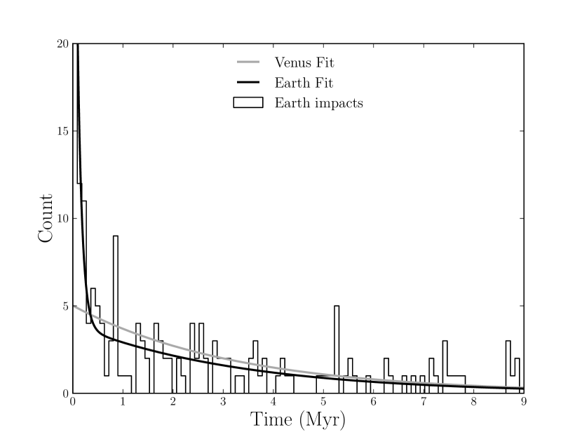
Figure 14: Post tidal distribution collision times of fragments with Venus and Earth. The number that collide with Earth as a function of time was fit to a double-exponential decay of the form $N_{E}(t)=N_{fast,E}\exp(t/\tau_{fast,E})+N_{slow,E}\exp(t/\tau_{slow,E})$ with $\tau_{fast,E}=0.09\pm 0.01$ Myr and $\tau_{slow,E}=3.3\pm 0.7$ Myr. Note that the first bin with 34 entries is truncated. The Venus impacts (not shown because they are similar in structure to the Earth impacts) were fit to a single-exponential decay of the form $N_{V}(t)=N_{slow,V}\exp(t/\tau_{slow,V})$ with $\tau_{slow,V}=3.3\pm 0.4$ Myr.

It is not surprising that the fraction of fragments that strike Earth is about $5\times$ higher than the fraction of NEOs that strike Earth as measured by Gladman et al. (2000) — since they were created at Earth they tend to come back to their point of origin. Indeed, there is a dramatic spike in the impact rate at Earth in the first 100,000 years following a catastrophic disruption (Fig. 14). Thus, if an NEO with $D>1\,\mathrm{km}$ ($H_{p}\lesssim 17.5$) suffers an s-class event near Earth about every 6,000 years (Richardson et al., 1998) then it is likely that Earth is continuously creating shrapnel that increases the impact collision risk above that measured for the dynamical background NEO population. Every catastrophic disruption produces many $<100$ m fragments that were not tracked in our work so that each event temporarily increases the density of small NEOs on Earth-like orbits for several tens of thousands of years. Many of them will collide with Earth and cause localized damage or, more optimistically, they would be good targets for future spacecraft missions due to their favorable orbits and low $v_{\infty}$.

The decay rate for impacts on Venus and Earth are identical after removing the ‘fast’ component due to impacts on Earth in the first 100 kyr. This ‘slow’ component of the impacts has a decay rate about $30\times$ longer than the fast component with a typical decay time of about 3.3 Myr. On this time scale the orbits of the fragments have a lot of time to evolve dynamically back into more typical NEO-like orbits.

4 Discussion

4.1 Future improvements

The coherence times of our simulated families differ by up to an order of magnitude due to the unique circumstances of each family’s post-disruption orbit. None of our families remained dynamically coherent for more than about 70,000 years and, depending on the size of the progenitor, the detectable lifetime is on the order of only thousands of years. An extensive quantitative study similar to this one but using a much larger sample of progenitors and fully exploring the phase space of rotation rates, shapes, pole orientations, etc., is required to draw a better picture of the evolution of tidally created NEO families. Such a study might be capable of identifying regions in NEO orbital element space where a family could remain clustered for long times and therefore be detectable on longer time scales. Indeed, our NEO cluster detection algorithm was applied by Schunová et al. (2012) over the entire NEO population. It might be modifiable to specifically examine the statistical significance of NEO clusters in the range of orbit elements most likely to contain young tidally disrupted NEO families. Combining the orbit element phase space search for NEO clusters with a taxonomic classification might provide a more statistically robust detection mechanism (Ivezić et al., 2002; Jewitt & Hsieh, 2006).

In §2.4 we mentioned that we ignored trailing losses in our NEO detection simulations and we can justify doing so because the relatively large $H<23$ NEOs considered in this analysis are usually detected far enough away that their apparent rate of motion on the sky plane is small. Extending our technique to smaller objects in the several- to hundred-meter size range would require an exquisite understanding of their detection efficiency as they will only be detected when they are bright enough during a very close approach to Earth — but under these circumstances their rate of motion on the sky will be high and they can escape detection due to trailing losses during the exposure time (e.g. Vereš et al., 2012). Trailing losses occur when fast moving asteroids leave trails on the detector so that the amount of flux per pixel decreases relative to the flux for a stationary object of the same intrinsic brightness. For example, trailing losses start to occur in the Pan-STARRS1 survey when objects move faster than about $0.5$ deg/day (Denneau et al., 2013). Detecting the small, trailed asteroids in the images will require more sophisticated image analysis techniques and a good measurement of their detection efficiency will be required to incorporate the small objects into an NEO cluster search algorithm.

4.2 Limits on s-class event frequency

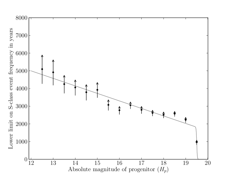
Figure 15: Lower limit on the interval between detectable family-producing s-class disruption events as a function of the progenitor’s absolute magnitude $H_{p}$. The central value on each data point is the formally calculated limit and the range of the arrow indicates the uncertainty on the limit due to the uncertainty on the lifetime of families produced at each progenitor’s absolute magnitude. The limit was fit to a function of the form $F_{S}=(F_{0}+m\,H_{p})/[1+\exp\{{(H_{p}-H_{limit})/H_{width}}\}]$ with $F_{0}=(10.1\pm 0.6)\times 10^{3}\,\mathrm{yr}$, $m=-424\pm 39\,\mathrm{yr}$/mag, $H_{limit}=19.5$ and $H_{width}=0.1$ mag (we do not provide the uncertainties for the last two parameters because they are much larger than the precision required to reproduce the fit shown on the figure).

Schunová et al. (2012) detected zero NEO families with fragments of $H<23$ which allows us to set observational limits on the s-class disruption frequency assuming 1) that all NEO families are created by s-class tidal disruptions and 2) ignoring the 33% contribution from Venus (i.e. assuming all tidal disruptions occur at Earth; see §2.2). Since the steady state number $N$ of detectable s-class families in the NEO population is the product of their flux $F$ (creation rate) and average detectable lifetime $L=\bar{\tau}_{det}$, we can set an observational lower limit on the creation rate of the tidally disrupted families $F_{S}$ (see Fig. 15).

At about the 90% confidence level a 1$\,\mathrm{km}$ NEO s-class disruption can take place no more frequently than once per $\sim 2,300\,\mathrm{yr}$ or an NEO family would already have been detected. We can not place a robust percentage on the confidence limit because we have not performed enough tidal disruption simulations with a realistic distribution of physical parameters. Furthermore, we have so far ignored the detailed contribution of s-class families to the NEO population by tidal disruption at Venus. For example, while we have estimated that Venus produces s-class families at about 33% of the rate produced by Earth the detectable lifetimes of those families is probably considerably shorter due to their larger mean distance from Earth so they probably make only a small contribution to the detectable number of NEO families.

Our lower limit on the disruption rate of 1 every $1,000\,\mathrm{yr}$ at $H_{p}=20$ corresponding to objects about $300\,\mathrm{m}$ in diameter, is about 6$\times$ times smaller than the predicted rate for $200\,\mathrm{m}$ NEOs of one every 6,200 years as calculated by Tóth et al. (2011) based on the SFD of Ivanov (2008). Our limit is about 3$\times$ smaller than the rate of one $300\,\mathrm{m}$ NEOs every 3,100 yr that we calculate based on the collision probability of NEOs with Earth (Bottke et al., 1994) assuming that the Earth’s impact cross-section is equivalent to a sphere with a radius 1.5$\times$ the Earth’s to allow for gravitational focussing and that tidal disruptions do not require impact.

In other words, it is unlikely that a tidally disrupted NEO cluster could be detected given the predicted rate and given our current cluster detection algorithms and observed set of NEOs. To detect such a cluster would require either luck, e.g. a recent tidal disruption of an NEO, or more sensitive NEO surveys to identify more and smaller objects. The problem with detecting more NEOs is that it increases the number of background objects at the same time as it increases the number of detected fragments from a disruption event and it is unclear how the Schunová et al. (2012) detection algorithm will perform in the presence of a larger background population.

4.3 Other evidence for disruptions and implications for asteroid space missions

It is possible that there already exists evidence of a population of asteroids created in a tidal disruption in the form of an enhancement in the number of small objects in Earth-like orbits (Rabinowitz et al., 1993) or the discrepancy between the observed (Mainzer et al., 2011) and predicted number (Bottke et al., 2002) of NEOs on low-inclination orbits. Both observations might be explained as enhancements due to a recent tidal disruption of NEOs by Earth.

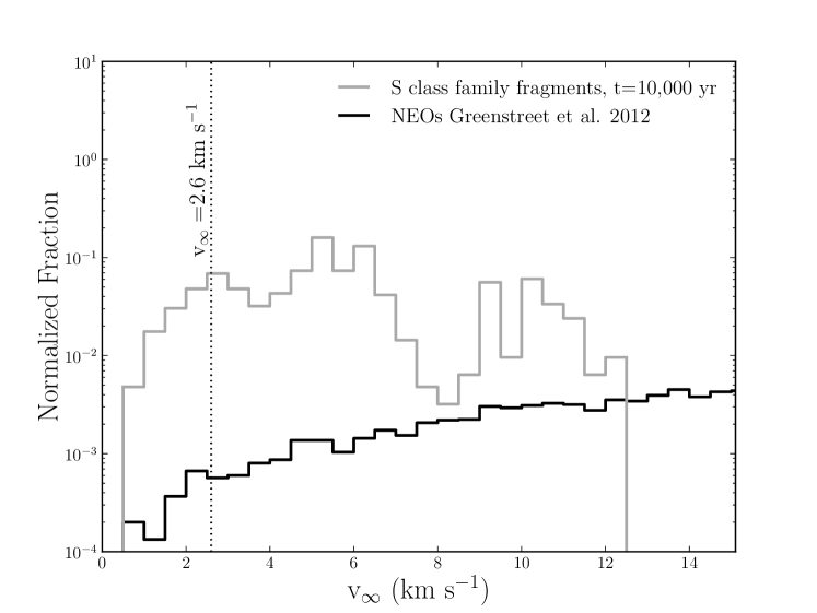
Figure 16: $v_{\infty}$ of all s-class family members 10,000 years after tidal disruption compared to the distribution for NEOs from Greenstreet et al. (2012). Roughly 10% of tidal disruption fragments have $v_{\infty}<2.6\,\mathrm{km}\,\mathrm{s}^{-1}$ as required for NASA’s Asteroid Retrieval mission compared to just 0.1% for the background (dynamical) NEO population. The latter distribution has a maximum at $v_{\infty}\sim 60\,\mathrm{km}\,\mathrm{s}^{-1}$.

We will concentrate on the small NEOs with $27<H<31$ in Earth-like orbits because they are of interest in NASA’s Asteroid Retrieval Mission (ARM) concept that seeks to bring a small heliocentric object into Earth orbit. The ARM initiative would like to target objects with $v_{\infty}<2.6\,\mathrm{km}\,\mathrm{s}^{-1}$. Assuming that we can extend the average SFD slope of $\alpha=0.55$ for s-class families to the size range of interest and using the average $\Delta H_{1}=1$ there are $\sim 2.6\times 10^{7}$ fragments in the ARM size range produced in the disruption of a single 1 km parent body. Roughly 10% of the fragments from an s-class tidal disruption meet the ARM $v_{\infty}$ threshold compared to only 0.1% of the overall NEO population (see Fig. 16). The $v_{\infty}$ distribution increases with time from disruption as the members dissipate into NEO orbit element space but many fragments will still fulfill the mission criterion. Thus, the tidal disruption of a single 1 km progenitor at Earth could generate $\sim 3\times 10^{6}$ ARM targets. The steady state population is about 1,200 ARM targets assuming that one 1 km diameter NEO tidally disrupts at Earth every 2,500 years.

Within the dynamical NEO population we expect $\sim 4\times 10^{8-9}$ NEOs in the same size range depending on the underlying NEO model (e.g. Brown et al., 2002; Harris, 2012) of which $\sim 0.1$% satisfy the ARM $v_{\infty}$ requirement yielding $\sim 4\times 10^{5-6}$ objects. The steady-state number of potential ARM targets created by tidal disruption is too low to explain the observed excess of small NEOs on Earth-like orbits but a disruption event within the past $\sim 10,000$ years might double the population of ARM targets in the NEO population and contribute to the explanation of the discrepancy between the Bottke et al. (2002) NEO model and observations such as those by Rabinowitz et al. (1993) and Mainzer et al. (2011).

5 Conclusion

We have shown that catastrophic tidal disruptions of NEOs as they pass close to Earth are capable of creating detectable NEO families. Our simulations suggest that the members of NEO families created by tidal disruptions are highly porous with a size-frequency distribution $\propto 10^{(0.55\pm 0.11)\,H}$, where the uncertainty is dominated by the systematic errors in our analysis.

The rapid dynamical evolution of the members of the tidally disrupted families results in their rapid dissipation so that they can only be identified by their orbital similarity for several tens of thousands of years with an average size-independent family coherence time of $\tau_{c}=(14.7\pm 0.6)\times 10^{3}\,\mathrm{yr}$. This value sets an upper limit on the family’s detectable lifetime $\tau_{det}$ — the time during which the family members may be detectable by current surveys and identified as statistically significant clusters in orbit element space. The detectability lifetime decreases from about 11,500 years for progenitors with absolute magnitudes of $H_{p}=13$ (about 10 km diameter) to about 5,000 years at $H_{p}=18$ (about 1 km diameter). This timescale is extremely short compared to main belt families that are detectable on Gyr timescales and probably explains why zero NEO families have been discovered to-date.

The fragments from a tidal disruption at Earth have a high probability of impacting Earth at future apparitions within about 100 kyr. It is possible that the creation rate of this kind of family is high enough that Earth is continuously creating shrapnel that increases the risk of collisions with Earth above the rate expected from the background dynamical NEO population.

The smallest parent body capable of producing an NEO family detectable with current surveys and our cluster search technique is $H_{p,max}\sim 20$ (for $\bar{\alpha}\sim 0.55$ and $\mkern 1.5mu\overline{\mkern-1.5mu\Delta H_{1}\mkern-1.5mu}\mkern 1.5mu\sim 1.0$) corresponding to asteroids of about 0.3 to 0.7 km in diameter depending on their albedo.

The null detection of NEO families by Schunová et al. (2012) allowed us to set a lower limit on the frequency of s-class NEO family producing events. We conclude that at about the 90% confidence level a $1\,\mathrm{km}$ NEO can disrupt and create a s-class family no more frequently than once per $\sim 2,300\,\mathrm{yr}$, or no more than once per $\sim 1,000\,\mathrm{yr}$ for the smallest possible detectable progenitor with $H_{p,max}\sim 20$. i.e.real NEO family would have been already detected Schunová et al. (e.g.  2012) if the rate were more frequent. These limits are a few times smaller than the theoretical expectations so we have not usefully constrained dynamical or disruption models. Instead, we have shown that the identification of tidally disrupted NEO families will be difficult unless new techniques are developed, or existing techniques are modified to search specifically for tidal disruptions. The combination of spectral similarity with orbital similarity may be fruitful at establishing statistically robust families under the assumption that the dust produced during the tidal disruption reaccumulates homegeneously on the fragments.

Nonetheless, every tidal disruption event is capable of producing a NEO ‘stream’ — up to several million fragments for a 1 km progenitor. We speculate that a relatively recent disruption event that is as-yet-unidentified with an NEO family may have contributed to the observed excess of objects on low-inclination orbits compared to the current model predictions. Such an event would create local orbit-element density enhancements of small NEOs in Earth-like orbits that would be excellent targets for future asteroid spacecraft exploration like the Asteroid Retrieval Mission (ARM) due to their low $v_{\infty}$ and associated low $\Delta v$.

Figure 12: Detectable lifetime of tidally disrupted NEO families as a function of the progenitor’s absolute magnitude $H_{p}$ with and without a cut in fragment size at $H_{frag,max}=23$. The detectability lifetime includes observational selection effects typical of all the NEOs in the known population as well as the efficiency of the cluster detection algorithm. The lifetime without the $H_{frag,max}$ cut was fit to a function of the form $\tau_{det}=(\tau_{0}+m\,H_{p})/\{1+\exp[{(H_{p}-H_{limit})/H_{width}}]\}$ with $(\tau_{0}=23.8\pm 1.5)\times 10^{3}$ years, $m=(-1.0\pm 0.1)\times 10^{3}$ years/mag, $H_{limit}=19.5$ and $H_{width}=0.1$. The fit with the $H_{frag,max}$ cut is almost identical. (We do not provide the uncertainties for the last two parameters because they are much larger than the precision required to reproduce the fit shown on the figure.)

References

- (1)
- Abe et al. (2006) Abe, S., Mukai, T., Hirata, N., Barnouin-Jha, O. S., Cheng, A. F., Demura, H., Gaskell, R. W., Hashimoto, T., Hiraoka, K., Honda, T., Kubota, T., Matsuoka, M., Mizuno, T., Nakamura, R., Scheeres, D. J. & Yoshikawa, M. (2006), ‘Mass and Local Topography Measurements of Itokawa by Hayabusa’, Science 312, 1344–1349.
- Asphaug et al. (1996) Asphaug, E., Benz, W., Ostro, S. J., Scheeres, D. J., de Jong, E. M., Suzuki, S. & Hudson, R. S. (1996), Disruptive Impacts into Small Asteroids, in ‘Bulletin of the American Astronomical Society, Vol. 28’, Vol. 28 of American Astronomical Society, DPS meeting #28, #10.31, p. 1102.
- Baer et al. (2011) Baer, J., Chesley, S. R. & Matson, R. D. (2011), ‘Astrometric Masses of 26 Asteroids and Observations on Asteroid Porosity’, Astronomical Journal 141, 143.
- Bottke et al. (1999a) Bottke, Jr., W. F., Richardson, D. C., Michel, P. & Love, S. G. (1999a), ‘1620 Geographos and 433 Eros: Shaped by Planetary Tides?’, Astronomical Journal 117, 1921–1928.
- Bottke et al. (1994) Bottke, W. F., J., Nolan, M. C., Greenberg, R. & Kolvoord, R. A. (1994), Collisional Lifetimes and Impact Statistics of Near-earth Asteroids, in T. Gehrels, M. S. Matthews & A. Schumann, eds, ‘Hazards due to comets and asteroids’, University of Arizona Press, pp. 336–357.
- Bottke et al. (1999b) Bottke, W. F., J., Richardson, D. C., Michel, P. & Love, S. G. (1999b), ‘1620 Geographos and 433 Eros: Shaped by Planetary Tides?’, The Astronomical Journal 117, 1921–1928.
- Bottke et al. (2002) Bottke, W. F., Morbidelli, A., Jedicke, R., Petit, J. M., Levison, H. F., Michel, P. & Metcalfe, T. S. (2002), ‘Debiased Orbital and Absolute Magnitude Distribution of the Near-Earth Objects’, Icarus 156(2), 399–433.
- Bottke et al. (2001) Bottke, W. F., Vokrouhlický, D., Brož, M., Nesvorný, D. & Morbidelli, A. (2001), ‘Dynamical spreading of asteroid families by the Yarkovsky effect.’, Science 294, 1693–1696.
- Brown et al. (2002) Brown, P., Spalding, R. E., ReVelle, D. O., Tagliaferri, E. & Worden, S. P. (2002), ‘The flux of small near-Earth objects colliding with the Earth’, Nature 420, 294–296.
- Brozović et al. (2011) Brozović, M., Benner, L. A. M., Taylor, P. A., Nolan, M. C., Howell, E. S., Magri, C., Scheeres, D. J., Giorgini, J. D., Pollock, J. T., Pravec, P., Galád, A., Fang, J., Margot, J.-L., Busch, M. W., Shepard, M. K., Reichart, D. E., Ivarsen, K. M., Haislip, J. B., Lacluyze, A. P., Jao, J., Slade, M. A., Lawrence, K. J. & Hicks, M. D. (2011), ‘Radar and optical observations and physical modeling of triple near-Earth Asteroid (136617) 1994 CC’, Icarus 216, 241–256.
- Chambers (1999) Chambers, J. E. (1999), ‘A hybrid symplectic integrator that permits close encounters between massive bodies’, Monthly Notices of the Royal Astronomical Society 304, 793–799.
- Chandrasekhar (1969) Chandrasekhar, S. (1969), The Silliman Foundation Lectures, New Haven: Yale University Press, chapter Ellipsoidal figures of equilibrium.
- Chesley & Spahr (2004) Chesley, S. R. & Spahr, T. B. (2004), Earth impactors: orbital characteristics and warning times, in M. J. S. Belton, T. H. Morgan, N. H. Samarasinha, & D. K. Yeomans , ed., ‘Mitigation of Hazardous Comets and Asteroids’, pp. 22–+.
- Denneau et al. (2013) Denneau, L., Jedicke, R., Grav, T., Granvik, M., Kubica, J., Milani, A., Vereš, P., Wainscoat, R., Chang, D., Pierfederici, F., Kaiser, N., Chambers, K. C., Heasley, J. N., Magnier, E. A., Price, P. A., Myers, J., Kleyna, J., Hsieh, H., Farnocchia, D., Waters, C., Sweeney, W. H., Green, D., Bolin, B., Burgett, W. S., Morgan, J. S., Tonry, J. L., Hodapp, K. W., Chastel, S., Chesley, S., Fitzsimmons, A., Holman, M., Spahr, T., Tholen, D., Williams, G. V., Abe, S., Armstrong, J. D., Bressi, T. H., Holmes, R., Lister, T., McMillan, R. S., Micheli, M., Ryan, E. V., Ryan, W. H. & Scotti, J. V. (2013), ‘The Pan-STARRS Moving Object Processing System’, Publications of the Astronomical Society of the Pacific 125, 357–395.
- Dohnanyi (1969) Dohnanyi, J. S. (1969), ‘Collisional Model of Asteroids and Their Debris’, Journal of Geophysical Research 74, 2531.
- Drummond (2000) Drummond, J. D. (2000), ‘The D-discriminant and Near-Earth Asteroid Streams’, Icarus 146(2), 453–475.
- Fu et al. (2005) Fu, H., Jedicke, R., Durda, D. D., Fevig, R. & Binzel, R. P. (2005), ‘Identifying near-Earth object families’, Icarus 178(2), 434–449.
- Fujiwara et al. (2006) Fujiwara, A., Kawaguchi, J., Yeomans, D. K., Abe, M., Mukai, T., Okada, T., Saito, J., Yano, H., Yoshikawa, M., Scheeres, D. J., Barnouin-Jha, O., Cheng, A. F., Demura, H., Gaskell, R. W., Hirata, N., Ikeda, H., Kominato, T., Miyamoto, H., Nakamura, A. M., Nakamura, R., Sasaki, S. & Uesugi, K. (2006), ‘The Rubble-Pile Asteroid Itokawa as Observed by Hayabusa’, Science 312, 1330–1334.
- Gladman et al. (2000) Gladman, B., Michel, P. & Froeschlé, C. (2000), ‘The Near-Earth Object Population’, Icarus 146, 176–189.
- Granvik (2009) Granvik, M. (2009), Pan-STARRS Survey for Near-Earth Objects, Planetary Defense Conference, IAA. CDROM.
- Granvik et al. (2012) Granvik, M., Vaubaillon, J. & Jedicke, R. (2012), ‘The population of natural Earth satellites’, Icarus 218, 262–277.
- Granvik et al. (2009) Granvik, M., Virtanen, J., Oszkiewicz, D. & Muinonen, K. (2009), ‘OpenOrb: Open-source asteroid orbit computation software including statistical ranging’, Meteoritics and Planetary Science 44, 1853–1861.
- Grav et al. (2011) Grav, T., Jedicke, R., Denneau, L., Chesley, S., Holman, M. J. & Spahr, T. B. (2011), ‘The Pan-STARRS Synthetic Solar System Model: A Tool for Testing and Efficiency Determination of the Moving Object Processing System’, Publications of the Astronomical Society of the Pacific 123, 423–447.
- Greenberg et al. (1994) Greenberg, R., Nolan, M. C., Bottke, W. F. J., Kolvoord, R. A. & Veverka, J. (1994), ‘Collisional history of Gaspra’, Icarus 107, 84.
- Greenstreet et al. (2012) Greenstreet, S., Ngo, H. & Gladman, B. (2012), ‘The orbital distribution of Near-Earth Objects inside Earth’s orbit’, Icarus 217, 355–366.
- Harris (1996) Harris, A. W. (1996), ‘The Rotation Rates of Very Small Asteroids: Evidence for ’Rubble Pile’ Structure’, Lunar and Planetary Science 27, 493.
- Harris (1998) Harris, A. W. (1998), ‘Evaluation of ground-based optical surveys for near-Earth asteroids’, Planetary and Space Science 46, 283–290.
- Harris (2012) Harris, A. W. (2012), The Value Of Enhanced Neo Surveys, in ‘AAS/Division for Planetary Sciences Meeting Abstracts’, Vol. 44 of AAS/Division for Planetary Sciences Meeting Abstracts, p. #305.08.
- Ivanov (2008) Ivanov, B. (2008), Size-Frequency Distribution of Asteroids and Impact Craters: Estimates of Impact Rate, p. 91.
- Ivezić et al. (2002) Ivezić, Ž., Lupton, R. H., Jurić, M., Tabachnik, S., Quinn, T., Gunn, J. E., Knapp, G. R., Rockosi, C. M. & Brinkmann, J. (2002), ‘Color Confirmation of Asteroid Families’, The Astronomical Journal 124, 2943–2948.
- Jedicke et al. (2003) Jedicke, R., Morbidelli, A., Spahr, T., Petit, J.-M. & Bottke, W. F. (2003), ‘Earth and space-based NEO survey simulations: prospects for achieving the spaceguard goal’, Icarus 161, 17–33.
- Jewitt & Hsieh (2006) Jewitt, D. & Hsieh, H. (2006), ‘Physical Observations of 2005 UD: A Mini-Phaethon’, The Astronomical Journal 132, 1624–1629.
- Jewitt & Li (2010) Jewitt, D. & Li, J. (2010), ‘Activity in Geminid Parent (3200) Phaethon’, The Astronomical Journal 140, 1519–1527.
- Kaiser et al. (2010) Kaiser, N., Burgett, W., Chambers, K., Denneau, L., Heasley, J., Jedicke, R., Magnier, E., Morgan, J., Onaka, P. & Tonry, J. (2010), The Pan-STARRS wide-field optical/NIR imaging survey, in L. M. Stepp, R. Gilmozzi & H. J. Hall, eds, ‘Ground-based and Airborne Telescopes III’, Vol. 7733, Proceedings of the SPIE, pp. 77330E–77330E–14.
- Kornoš et al. (2009) Kornoš, L., Tóth, J. & Vereš, P. (2009), ‘Release of meteoroids from asteroids by Earth’s tides’, Contributions of the Astronomical Observatory Skalnate Pleso 39, 18–24.
- Leinhardt et al. (2000) Leinhardt, Z. M., Richardson, D. C. & Quinn, T. (2000), ‘Direct N-body Simulations of Rubble Pile Collisions’, Icarus 146, 133–151.
- Love & Ahrens (1996) Love, S. G. & Ahrens, T. J. (1996), ‘Catastrophic Impacts on Gravity Dominated Asteroids’, Icarus 124, 141–155.
- Mainzer et al. (2011) Mainzer, A., Grav, T., Bauer, J., Masiero, J., McMillan, R. S., Cutri, R. M., Walker, R., Wright, E., Eisenhardt, P., Tholen, D. J., Spahr, T., Jedicke, R., Denneau, L., DeBaun, E., Elsbury, D., Gautier, T., Gomillion, S., Hand, E., Mo, W., Watkins, J., Wilkins, A., Bryngelson, G. L., Del Pino Molina, A., Desai, S., Gómez Camus, M., Hidalgo, S. L., Konstantopoulos, I., Larsen, J. A., Maleszewski, C., Malkan, M. A., Mauduit, J.-C., Mullan, B. L., Olszewski, E. W., Pforr, J., Saro, A., Scotti, J. V. & Wasserman, L. H. (2011), ‘NEOWISE Observations of Near-Earth Objects: Preliminary Results’, Astrophysical Journal 743, 156.
- Melosh & Stansberry (1991) Melosh, H. J. & Stansberry, J. A. (1991), ‘Doublet craters and the tidal disruption of binary asteroids’, Icarus 94, 171–179.
- Melosh & Whitaker (1994) Melosh, H. J. & Whitaker, E. A. (1994), ‘Lunar crater chains’, Nature 369, 713–714.
- Michel et al. (2000) Michel, P., Migliorini, F., Morbidelli, A. & Zappalà, V. (2000), ‘The population of Mars-crossers: Classification and dynamical evolution.’, Icarus 145, 332–347.
- Migliorini et al. (1998) Migliorini, F., Michel, P., Morbidelli, A., Nesvorný, D. & Zappal à, V. (1998), ‘Origin of Earth-crossing asteroids: A quantitative simulation.’, Science 281, 2022–2024.
- Milani et al. (2012) Milani, A., Knezevic, Z., Farnocchia, D., Bernardi, F., Jedicke, R., Denneau, L. & PS1 Science Collaboration (2012), ‘Identification of Known Objects in Solar System Surveys’, LPI Contributions 1667, 6214.
- Nesvorný et al. (2010) Nesvorný, D., Bottke, W. F., Vokrouhlický, D., Chapman, C. R. & Rafkin, S. (2010), ‘Do planetary encounters reset surfaces of near Earth asteroids?’, Icarus 209, 510–519.
- Nesvorny et al. (2006) Nesvorny, D., Vokrouhlicky, D. & Bottke, W. F. (2006), ‘The Breakup of a Main-Belt Asteroid 450 Thousand Years Ago’, Science 312, 1490.
- Nugent et al. (2012) Nugent, C. R., Margot, J. L., Chesley, S. R. & Vokrouhlický, D. (2012), ‘Detection of Semimajor Axis Drifts in 54 Near-Earth Asteroids: New Measurements of the Yarkovsky Effect’, Astronomical Journal 144, 60.
- O’Brien & Greenberg (2005) O’Brien, D. P. & Greenberg, R. (2005), ‘The collisional and dynamical evolution of the main-belt and NEA size distributions’, Icarus 178, 179–212.
- Ohtsuka et al. (2008) Ohtsuka, K., Arakida, H., Ito, T., Yoshikawa, M. & Asher, D. J. (2008), ‘Apollo Asteroid 1999 YC: Another Large Member of the PGC?’, Meteoritics and Planetary Science Supplement 43, 5055.
- Ohtsuka et al. (2006) Ohtsuka, K., Sekiguchi, T., Kinoshita, D., Watanabe, J.-I., Ito, T., Arakida, H. & Kasuga, T. (2006), ‘Apollo asteroid 2005 UD: split nucleus of (3200) Phaethon?’, Astronomy and Astrophysics 450, L25–L28.
- Ostro et al. (2006) Ostro, S. J., Margot, J.-L., Benner, L. A. M., Giorgini, J. D., Scheeres, D. J., Fahnestock, E. G., Broschart, S. B., Bellerose, J., Nolan, M. C., Magri, C., Pravec, P., Scheirich, P., Rose, R., Jurgens, R. F., De Jong, E. M. & Suzuki, S. (2006), ‘Radar Imaging of Binary Near-Earth Asteroid (66391) 1999 KW4’, Science 314, 1276–1280.
- Ostro et al. (1995) Ostro, S. J., Rosema, K. D., Hudson, R. S., Jurgens, R. F., Giorgini, J. D., Winkler, R., Yeomans, D. K., Choate, D., Rose, R., Slade, M. A., Howard, S. D. & Mitchell, D. L. (1995), ‘Extreme elongation of asteroid 1620 Geographos from radar images’, Nature 375, 474–477.
- Pravec & Harris (2000) Pravec, P. & Harris, A. W. (2000), ‘Fast and Slow Rotation of Asteroids’, Icarus 148, 12–20.
- Pravec et al. (2002) Pravec, P., Harris, A. W. & Michalowski, T. (2002), Asteroid Rotations, in W. Bottke, A. Cellino, P. Paolicchi & R. P. Binzel, eds, ‘Asteroids III’, University of Arizona Press, pp. 113–122.
- Rabinowitz et al. (1993) Rabinowitz, D. L., Gehrels, T., Scotti, J. V., McMillan, R. S., Perry, M. L., Wisniewski, W., Larson, S. M., Howell, E. S. & Mueller, B. E. A. (1993), ‘Evidence for a near-Earth asteroid belt’, Nature 363, 704–706.
- Richardson et al. (1998) Richardson, D. C., Bottke, W. F. & Love, S. G. (1998), ‘Tidal Distortion and Disruption of Earth-Crossing Asteroids’, Icarus 134, 47–76.
- Richardson et al. (2002) Richardson, D. C., Leinhardt, Z. M., Melosh, H. J., Bottke, W. F., J. & Asphaug, E. (2002), Gravitational Aggregates: Evidence and Evolution, in W. Bottke, A. Cellino, P. Paolicchi & R. P. Binzel, eds, ‘Asteroids III’, University of Arizona Press, pp. 501–515.
- Roche (1849) Roche, E. (1849), La figure d’une masse fluide soumise à l’attraction d’un point èloignè, in ‘Acadèmie des sciences de Montpellier: Mèmoires de la section des sciences.’, Vol. 1, Acadèmie des sciences de Montpellier, pp. 243–262.
- Saito et al. (2006) Saito, J., Miyamoto, H., Nakamura, R., Ishiguro, M., Michikami, T., Nakamura, A. M., Demura, H., Sasaki, S., Hirata, N., Honda, C., Yamamoto, A., Yokota, Y., Fuse, T., Yoshida, F., Tholen, D. J., Gaskell, R. W., Hashimoto, T., Kubota, T., Higuchi, Y., Nakamura, T., Smith, P., Hiraoka, K., Honda, T., Kobayashi, S., Furuya, M., Matsumoto, N., Nemoto, E., Yukishita, A., Kitazato, K., Dermawan, B., Sogame, A., Terazono, J., Shinohara, C. & Akiyama, H. (2006), ‘Detailed Images of Asteroid 25143 Itokawa from Hayabusa’, Science 312, 1341–1344.
- Scheeres et al. (2002) Scheeres, D. J., Durda, D. D. & Geissler, P. E. (2002), ‘The Fate of Asteroid Ejecta’, Asteroids III pp. 527–544.
- Schunová et al. (2012) Schunová, E., Granvik, M., Jedicke, R., Gronchi, G., Wainscoat, R. & Abe, S. (2012), ‘Searching for the first near-Earth object family’, Icarus 220, 1050–1063.
- Solem & Hills (1996) Solem, J. C. & Hills, J. G. (1996), ‘Shaping of Earth-Crossing Asteroids by Tidal Forces’, Astronomical Journal 111, 1382.
- Southworth & Hawkins (1963) Southworth, R. B. & Hawkins, G. S. (1963), ‘Statistics of meteor streams’, Smithsonian Contributions to Astrophysics 7, 261–285.
- Stuart (2003) Stuart, J. S. (2003), Observational Constraints on the Number, Albedos, Sizes, and Impact Hazards of the Near-Earth Asteroids, PhD thesis, MASSACHUSETTS INSTITUTE OF TECHNOLOGY.
- Tóth et al. (2011) Tóth, J., Vereš, P. & Kornoš, L. (2011), ‘Tidal disruption of NEAs - a case of Příbram meteorite’, Monthly Notices of the Royal Astronomical Society 415, 1527–1533.
- Vereš et al. (2012) Vereš, P., Jedicke, R., Denneau, L., Wainscoat, R., Holman, M. J. & Lin, H.-W. (2012), ‘Improved Asteroid Astrometry and Photometry with Trail Fitting’, Publications of the Astronomical Society of the Pacific 124, 1197–1207.
- Walsh & Richardson (2006) Walsh, K. J. & Richardson, D. C. (2006), ‘Binary near-Earth asteroid formation: Rubble pile model of tidal disruptions’, Icarus 180(1), 201–216.
- Walsh & Richardson (2008) Walsh, K. J. & Richardson, D. C. (2008), ‘A steady-state model of NEA binaries formed by tidal disruption of gravitational aggregates’, Icarus 193(2), 553–566.
- Warner et al. (2009) Warner, B. D., Harris, A. W. & Pravec, P. (2009), ‘The asteroid lightcurve database’, Icarus 202, 134–146.
- Whipple (1983) Whipple, F. L. (1983), ‘1983 TB and the Geminid Meteors’, IAU Circ. 3881, 1.
- Yeomans et al. (1997) Yeomans, D. K., Barriot, J.-P., Dunham, D. W., Farquhar, R. W., Giorgini, J. D., Helfrich, C. E., Konopliv, A. S., McAdams, J. V., Miller, J. K., Owen, Jr., W. M., Scheeres, D. J., Synnott, S. P. & Williams, B. G. (1997), ‘Estimating the Mass of Asteroid 253 Mathilde from Tracking Data During the NEAR Flyby’, Science 278, 2106.
- Zavodny et al. (2008) Zavodny, M., Jedicke, R., Beshore, E. C., Bernardi, F. & Larson, S. (2008), ‘The orbit and size distribution of small Solar System objects orbiting the Sun interior to the Earth’s orbit’, Icarus 198, 284–293.