Accurate water maser positions from HOPS

Abstract

We report on high spatial resolution water maser observations, using the Australia Telescope Compact Array, towards water maser sites previously identified in the H₂O southern Galactic Plane Survey (HOPS). Of the 540 masers identified in the single-dish observations of Walsh et al. (2011), we detect emission in all but 31 fields. We report on 2790 spectral features (maser spots), with brightnesses ranging from 0.06 Jy to 576 Jy and with velocities ranging from $-238.5$ to +300.5 km s^-1. These spectral features are grouped into 631 maser sites. We have compared the positions of these sites to the literature to associate the sites with astrophysical objects. We identify 433 (69 per cent) with star formation, 121 (19 per cent) with evolved stars and 77 (12 per cent) as unknown. We find that maser sites associated with evolved stars tend to have more maser spots and have smaller angular sizes than those associated with star formation. We present evidence that maser sites associated with evolved stars show an increased likelihood of having a velocity range between 15 and 35 km s^-1 compared to other maser sites. Of the 31 non-detections, we conclude they were not detected due to intrinsic variability and confirm previous results showing that such variable masers tend to be weaker and have simpler spectra with fewer peaks.

1 Introduction

Water (H₂O) masers were discovered towards Orion, Sgr B2 and W49 by Cheung et al. (1969) in the J${}_{\rm K_{a},K_{c}}=6_{1,6}\rightarrow 5_{2,3}$ spectral line at 22.235 GHz. All three of these targets are regions of high mass star formation (HMSF) in our Galaxy. Since their discovery, extensive work on H₂O masers has shown that although they are commonly associated with regions of HMSF (eg. Genzel & Downes 1977; Forster & Caswell 1999), H₂O masers are also found associated with sites of low mass star formation (eg. Dickinson, Strom & Kojoian 1974; Claussen et al. 1996), late M-type stars (Dickinson, 1976), planetary nebulae (Miranda et al., 2001), Mira variables (Hinkle & Barnes, 1979), asymptotic giant branch (AGB) stars (Barlow et al., 1996) and the centres of active galaxies (Claussen et al., 1984).

Much of the previous work on H₂O masers has been targeted on regions likely to show masers (eg. Forster & Caswell (1989); Breen & Ellingsen (2011); Comoretto et al. (1990), but this creates a possible bias whereby the full population of masers may not be seen. While it is clear that H₂O masers are associated with many different astrophysical objects, it is not clear the proportion of masers found towards each type of object. Knowing the proportions will yield a better understanding of the underlying populations and characteristics of the astrophysical objects.

In order to reduce biases associated with targeted surveys, the H₂O southern Galactic Plane Survey (HOPS) was conducted (Walsh et al., 2011). HOPS surveyed 100 square degrees of the southern and inner Galactic plane between Galactic longitudes of 290^∘ and 30^∘ and Galactic latitudes of $-0.5^{\circ}$ and $+0.5^{\circ}$, with a detection limit typically between 1 and 2 Jy. They detected 540 sites of H₂O maser emission, including 334 new detections. The observations were performed with the Mopra radio telescope, which is well designed to detect multiple bright spectral lines simultaneously, but is limited by a spatial resolution of about 2′. This spatial resolution is insufficient to unambiguously identify the source of the maser emission: higher spatial resolution observations are needed.

Masers are commonly found in small groups, referred to as maser sites. Each maser site consists of a number of maser spots, where each maser spot corresponds to a single peak in the maser spectrum and is usually considered to arise in a single, well-defined position. H₂O maser spots are typically resolved only on VLBI baselines, with physical sizes of tens of AU, or smaller (eg. Richards, Elitzur & Yates 2011). H₂O maser sites are rarely distributed over more than a few arcseconds and are typically smaller than one arcsecond across (Forster & Caswell, 1989). The relative orientation and kinematics of maser spots within a maser site, when observed at high resolution, can delineate outflows in regions of star formation (eg. Titmarsh et al. 2013; Bartkiewicz et al. 2011; Claussen et al. 1996) and evolved stars (eg. Imai et al. 2013; Walsh et al. 2009). Thus, high spatial resolution (ie. arcsecond) observations are required to precisely locate the maser sites, which helps identify the associated astrophysical object. High spatial resolution observations are also required to map the morphology of maser spots within a maser site or place stringent upper limits on the extent of the masers. In order to address these issues, we have observed those masers detected in HOPS with the Australia Telescope Compact Array (ATCA) at high spatial resolution.

2 Observations and data analysis

Observations were made with the ATCA during three sessions: from 2011 March, 13th to 23rd, on 2012 April 2nd and from 2012 May 25th to 31st. Configurations for the three sessions were 1.5A, H168 and 6D, respectively. The different configurations, together with elongated beams for observations close to declination 0 degrees, mean that the synthesised beam size varies. The smallest beam is 0.55 $\times$ 0.35 arcsec and the largest beam is 14.0 $\times$ 10.2 arcsec. When observing with the ATCA at declinations close to zero, the predominantly east–west baselines of the ATCA mean that the uv plane is poorly sampled along the declination axis, resulting in larger positional errors (ie. elongated beams) in this direction. Observational pointing centres were determined based on the H₂O maser detections listed in Table 2 of Walsh et al. (2011). Each target was observed typically using six snapshot observations of duration two minutes each, giving a typical on-source integration time of 12 minutes.

Primary flux calibration was done using the standard flux calibrator PKS B1934$-$638, bandpass calibration was performed using PKS B1253$-$055. Phase calibrators were chosen to be within 7 degrees of each target observation and the phase calibrators were monitored every 20 minutes. Pointing calibration was also performed on the phase calibrator every 80 minutes.

The Compact Array Broadband Backend (CABB) was used to collect data, using the 64M-32k mode. One zoom band was centred at 22.235 GHz, with bandwidth of 64 MHz and 2048 channels. This is equivalent to a velocity coverage of 863 km s^-1 and channel separation of 0.42 km s^-1. Edge channels were masked out during the data reduction process. The velocity coverage over which maser emission was searched was approximately $-400$ to $+400$ km s^-1in the Local Standard of Rest (LSR) reference frame. This velocity range is sufficient to cover velocities expected from Galactic rotation (up to $\pm 200$ km s^-1; Dame, Hartmann & Thaddeus 2001), but may miss some extremely high velocity maser spots.

The data were processed using miriad standard data reduction routines to produce cleaned and restored data cubes that are corrected for the primary beam response. The cubes were then searched (over the area of the primary beam) for maser emission. In order to manage the large volume of data and search within a reasonable amount of time, the following method was used to identify masers:

1. The full data cube was binned in three velocity channels to produce a binned cube. This binned cube is fine tuned to detect maser spots that have a characteristic line width close to the binned channel width of 1.2 km s^-1, based on our Mopra HOPS spectra (Walsh et al., 2011), maximising the sensitivity to detect masers.

2. A peak intensity map (in miriad a moment $-$2 map) was created from each of the full cube and binned cube.

3. Both peak intensity maps were searched by eye for bright spots, which are the signatures of masers.

4. Any maser candidate identified in the peak intensity maps was then scrutinised in the full data cube. With a sparse sampling of the uv-plane in these observations, together with often very bright maser spots, it is quite common that peaks in the peak intensity maps correspond to sidelobe artifacts. These can be discriminated from real maser spots by visually checking their appearance in the full data cube. A real maser spot will usually be seen as the brightest feature in the cube over its velocity range.

In our experience (Walsh et al., 2012), the above manual method of searching for and characterising features is less time consuming and at least as accurate as an automated method. Once maser spots have been identified, their positions are determined in the following way: The channels over which the maser spot are detected are used to form an integrated intensity map, giving the highest signal-to-noise ratio for that maser spot and hence the most accurate position. The miriad task imfit is used to fit the integrated intensity map and determine both the position and relative uncertainty in the position of the maser spot. The peak flux density and peak velocity of a maser spot are both determined from the peak channel in the spectrum of the maser spot.

The absolute uncertainty in maser positions depends on the phase noise during the observations, which is related to the distance to the phase calibrator, as well as the weather conditions and so is not precisely determined. We adopt a typical value for the absolute positional uncertainty of 1 arcsec, based on previous H₂O maser work with the ATCA by Breen et al. (2010) who found absolute positional uncertanties between 0.5 and 2 arcsec. The relative positional uncertainty between maser spots detected in the same observation can be more accurate than the absolute uncertainty, which allows us to compare the distributions of spots within a site on smaller scales than the absolute uncertainty, but does not allow us to compare the relative positions of masers with other datasets (eg GLIMPSE; Benjamin et al. 2003; Churchwell et al. 2009, as described below) to better than 1 arcsec.

The noise in the data varies depending on a number of factors including the array configuration used, the number of snapshots in each observation and the phase noise (as mentioned above). The presence of strong sources can also affect the noise through the limited dynamic range of the data. For each spectrum, we have determined the rms noise level by using channels in the velocity range of $-400$ to $-300$ km s^-1, where we do not expect to find any real emission. The distribution of rms noise levels is shown in Figure 1. The distribution shows a large range of noise levels from 6.5 mJy to 1.7 Jy, but with 90% of noise levels in the range 15 mJy to 167 mJy. The peak of the distribution is at 17 mJy and the median is 36 mJy.

Figure 1: Distribution of rms noise levels in the maser spectra. The noise is based on the data within each spectrum between -400 and -300 km s^-1. The peak of the distribution is at 17.5 mJy, with a median of 36 mJy.

3 Results

In total, we detect 2790 maser spots, with the brightest being 576 Jy and weakest being 0.06 Jy. The most redshifted maser spot is detected at +300.5 km s^-1 and the most blueshifted is detected at $-238.5$ km s^-1. Given the velocity range of $\pm$ 400 km s^-1 that we searched for masers, we do not expect that many extremely high velocity maser spots were missed. The distributions of maser spot brightnesses and velocities are shown in Figure 2. The distribution of peak flux densities shows a peak at 1.1 Jy with a median of 1.4 Jy. The reason for the drop in the number of maser peak flux densities below this is likely due to the limitation in detecting masers close to the noise level, as shown by the $3\times$ rms level shaded region in Figure 2.

We did not detect any masers towards 31 pointing centres in these observations. The list of non-detection pointing centres is given in Table 1 and are discussed further in §4.3.

In Figure 3, we show the distribution of angular distances to the nearest neighbour for each maser spot. Note that we do not plot any separations greater than 30 arcsec, as we consider separations greater than this distance due to chance alignments. From this distribution, we can see that the nearest neighbours are almost always within a few arcseconds of each other. This is because the maser spots are typically clustered within maser sites. It is important to categorise maser spots into sites, where the sites can be considered as associated with a single astrophysical object. We therefore use the distribution shown in Figure 3 as a way to define an angular size of maser sites. We choose an upper limit of 4 arcsec to the size of a maser site, which will apply to 94 per cent of maser spots and is equivalent a linear size of about 0.1 pc at a distance of 5 kpc. We caution that this maser site size is somewhat arbitrary for a number of reasons: It is based on an angular size, rather than a linear size and thus does not take into account the distance to the site. The size limit may well include more than one unrelated maser site along the line of sight. For example, there may be multiple young stellar objects within a tight cluster that each have their own maser site. The size limit may artificially break up masers with a single common origin, but separated by more then 4 arcsec on the sky. For example, a single maser site may encompass maser spots that occur in both lobes of an outflow associated with a single star. Forster & Caswell (1989) observed a number of H₂O maser sites associated with known star forming sites. They found the median extent of their maser sites was 9 mpc and with 63 per cent of maser sites smaller than 100 mpc. If a 100 mpc maser site was at a near distance of 3 kpc, it would appear 6.7 arcsec across. Using the median size of 9 mpc at the same distance, a maser site would appear 0.6 arcsec across. Thus, even at a very close distance to us, most typical maser sites would not be broken up using our criteria.

With the above-mentioned caveats in mind, we still consider the size upper limit a simple and practical guideline to define maser sites. Note that we treat G000.677$-$0.028 as a special case. This is the well-known star forming region Sgr B2 and exhibits maser spots spread over a wide area that we classify together as a single maser site, even though they are likely to have multiple powering sources. This is because there does not appear any clear, consistent way to break up these maser spots into multiple maser sites.

We identify 631 maser sites and in Table 2, we present data on maser spots, which are separated into their maser sites. In column 1, we assign a name to each maser spot, based on the Galactic coordinates of the brightest maser spot in the maser site, plus a letter (or letters) to identify each maser spot within the maser site. Spots are labelled sequentially, based on their relative radial velocity. In Figure 4, we show the distribution of the number of maser spots within a maser site. We find that most maser sites have either 1, 2 or 3 maser spots, but there are a small number of maser sites with many maser spots, up to 61 for the case of G000.677$-$0.028, which, as mentioned above, is a special case. The next richest maser site is G021.797$-$0.127, with 59 maser spots.

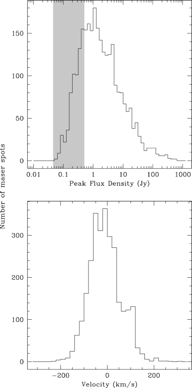
Figure 2: Distributions of general maser spot properties. (Top) The distribution of maser spot peak brightnesses is shown. The shaded area represents the range of $3\times{\rm rms}$ noise levels for 90 per cent of the data. (Bottom) The distribution of maser spot peak velocities is shown.

Figure 3: Distribution of the angular distance to the nearest neighbour for each maser spot. This distribution quickly falls off with increasing angular distance, showing that maser spots are typically distributed within small maser sites that are rarely more than a few arcseconds across.

Figure 4: The distribution of the number of maser spots within a maser site. Most maser sites contain 1, 2 or 3 maser spots. The most numerous maser site (G000.677$-$0.028, also known as Sgr B2) has 61 maser spots.

Table 1: List of pointing centres which show masers in Walsh et al. (2011) but were not detected in these observations. The reason for these non-detections is most likely due to intrinsic variability, making the masers undetectable in these observations.

G000.53+0.18 G018.16+0.39 G315.23$-$0.11 G001.17$-$0.04 G018.61$-$0.08 G315.93+0.05 G002.93+0.28 G291.79+0.39 G331.86+0.06 G005.37+0.05 G301.35+0.02 G333.46$-$0.16 G006.09$-$0.12 G301.76+0.29 G337.88$-$0.11 G012.94$-$0.04 G305.01+0.43 G338.17$-$0.07 G013.46+0.22 G308.70$-$0.00 G339.75+0.10 G014.03$-$0.31 G309.29$-$0.47 G342.63$-$0.09 G015.54$-$0.13 G314.41+0.05 G359.42+0.32 G016.28+0.42 G314.98+0.03 G017.98+0.24 G315.22$-$0.25

Table 2: Details of maser spots, based on ATCA observations. The first column lists the name of the maser spot, which is derived from the Galactic coordinates of the brightest peak, followed by a letter (or letters) to denote the sequence of maser spots in the spectrum. An asterisk (*) is used to identify the brightest maser spot for those maser sites with more than one spot. The second and third columns give the coordinates of the maser spot. The fourth column lists the spot peak flux density. The fifth column lists the velocity at the peak. The sixth and seventh columns give the relative uncertainty of the position, together with the orientation of the major axis uncertainty in the eigth column. The ninth and tenth columns list the major and minor axes of the synthesized beam, respectively. The full table is available online.

Name	RA	Dec.	Peak	Peak	Relative Uncertainty in Position			Synthesized Beam
	(J2000)	(J2000)	Flux	Velocity	Major	Minor	Position	Major	Minor
	(${}^{\circ\>\prime\>\prime\prime}$)	(${}^{\circ\>\prime\>\prime\prime}$)	Density	(km s-1)	Axis	Axis	Angle	Axis	Axis
			(Jy)		(″)	(″)	(∘)	(″)	(″)
G000.055$-$0.211A	17:46:34.570	$-$28:59:58.174	0.16	+08.8	0.100	0.038	$-$0.6	1.11	0.42
G000.055$-$0.211B*	17:46:34.570	$-$28:59:58.111	0.74	+13.7	0.048	0.018	$-$0.6	1.11	0.42
G000.055$-$0.211C	17:46:34.569	$-$28:59:58.015	0.24	+16.2	0.080	0.030	$-$0.6	1.11	0.42
G000.055$-$0.211D	17:46:34.571	$-$28:59:57.998	0.19	+19.8	0.083	0.032	$-$0.6	1.11	0.42
G000.306$-$0.170A	17:47:00.603	$-$28:45:45.724	1.56	+02.0	0.040	0.017	$-$4.7	1.09	0.45
G000.306$-$0.170B*	17:47:00.603	$-$28:45:45.740	37.9	+06.7	0.033	0.014	$-$4.7	1.09	0.45
G000.306$-$0.170C	17:47:00.604	$-$28:45:45.747	4.95	+09.7	0.030	0.013	$-$4.7	1.09	0.45

3.1 Maser site images

In Figure 5, we present images for each maser site distribution. For each maser site, we present the following: The top panel shows the spectrum at full resolution, including all the maser spots in the site. For each maser spot, a velocity range is shaded according to the channels over which emission is seen from that maser spot. We choose to shade velocity ranges like this because occasionally sidelobes from nearby maser sites may cause peak or dip artifacts in the spectrum that should not be interpreted as maser spots associated with the current maser site. Thus, only the shaded parts of the spectrum are relevant to the maser site shown in the Figure. In some spectra, there are darker-shaded velocity ranges, which indicate overlap between velocities of two maser spots that are spatially separated.

The bottom panel shows a 6′$\times$3′ area containing a 3-colour GLIMPSE (Benjamin et al., 2003; Churchwell et al., 2009) image, based on bands 1 for blue, 2 for green and 4 for red, with band wavelengths of 3.6, 4.5 and 8.0 $\mu$m, respectively. Note that for masers in the Galactic longitude range of 290–295^∘ the 3-colour image is made from MSX (Egan & Price, 1996) data, with band A for blue, band D for green and band E for red, with band wavelengths of 8.3, 14.7 and 21.3 $\mu$m, respectively. MSX data is used in this Galactic longitude range because this range is outside the GLIMPSE survey area. The image is centred on the maser site. All maser spots that were detected within this field of view are shown as black plus symbols, with white borders. Note that maser spots that are not part of the current maser site are also included in the lower panel so that the relative locations of all maser sites within the field of view can be seen. A scale bar of length 30 arcsec is presented in the lower-left corner of this panel. In the centre of the panel is a white box that represents the field of view shown in the middle-left panel.

The middle-left panel shows a zoomed-in region around the maser site. This region is a square with 21.6 arcsec sides. The same 3-colour image as the bottom panel is used as the background. The positions of maser spots within the maser site are shown as black plus symbols with white borders. Note that this panel shows only maser spots that are associated with this maser site. Therefore the maser spots in this panel and the bottom panel can be compared to decide which ones are associated with this maser site and which are not. A scale bar of 1 arcsec in length is presented in the bottom-left corner of the panel to illustrate a representative absolute positional uncertainty for the maser spots. Note that this scale bar is equivalent to the absolute positional error of the masers. The centre of this panel contains a white box, which represents the size of the zoomed area shown in the middle-right panel. The size of the middle-right panel is determined by the size of the maser site plus the errors on the maser spots, which may be very small or indeed larger than the middle-left panel. Thus, the white box is not always visible.

The middle-right panel presents a zoomed in region that contains the positions and relative error ellipses of all maser spots for this maser site. In this panel, each maser spot is represented either with a coloured ellipse or a coloured plus symbol. The plus symbol is used when the size of the ellipse would be too small to see easily. The position of the ellipse represents the fitted position of the maser spot. The major and minor axes, as well as the position angle, of the ellipse represent the relative positional uncertainty of the maser spots, derived from the miriad task imfit. The colour of the ellipse represents the peak velocity of the maser spot, according to the velocity colour-bar shown at the bottom of this panel. Ellipses are plotted such that smaller ellipses are on top of larger ones. Thus, at least some part of every ellipse will be visible in this panel. A scale bar is presented in the lower-left corner of this panel. Note that no absolute coordinates are presented in this panel because the absolute position is determined only to within 1 arcsec at best and this panel shows relative offsets of maser spot positions that are typically on much smaller scales than this.

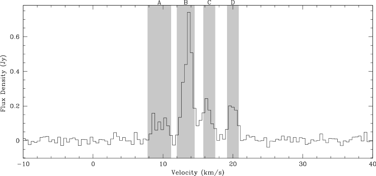
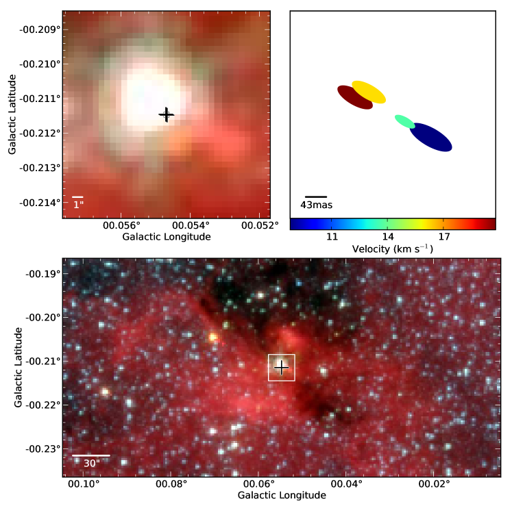
Figure 5: G000.055$-$0.211. Refer to §3.1 for a full description of the Figure. The full figure is available online.

4 Discussion

4.1 Maser site identification

An untargeted survey of water maser sites over a large section of the Galactic Plane allows us, for the first time, to carefully assess the relative occurrence of water masers towards different astrophysical objects. We note that even though Walsh et al. (2011) performed an untargeted survey, it is still flux limited and the area of the survey is limited in Galactic latitude. These factors may affect our detection statistics, which are discussed further below. We wish to determine the proportion of our detected water maser sites that are associated with sites of star formation, compared to those associated with evolved stars. For some maser sites we can use associations with reliable tracers of star formation (eg. class II methanol maser sites; Walsh et al. 1998) or evolved stars (eg. double-horned 1612 MHz OH maser profiles; Sevenster et al. 1997). However, for other maser sites, a clear assocation may not be evident. Therefore, we use a variety of methods to assign each maser site (where possible) to either a star formation or evolved star association. We caution that whilst we expect our classifications to be highly reliable, it is possible that a small number of our assignments are incorrect.

In Table 3, we list each maser site, together with information on associations with methanol maser sites, thermal ammonia emission, Red MSX Source (RMS) associations (Lumsden et al., 2013), previously detected sources, based on Walsh et al. (2011; hereafter Paper I) and features seen in the GLIMPSE images, shown in Figure 5. We use this information, as well as information from other sources in the literature, to assign each maser site as star formation, evolved star or unknown, based on the following method:

1. A H₂O maser site was assigned to star formation if the position is close to a class II methanol maser site. The distance between H₂O and methanol maser sites was chosen to be large enough to include the angular size of any water maser site (up to 4 arcsec). It was also chosen so that the Galactic coordinates of both maser sites could be directly compared: coordinates are quoted to the nearest 0.001 degree (3.6 arcsec) and so an association between maser sites is made when there is at most 0.001 degrees difference in both coordinates, equivalent to an angular separation of 5.1 arcsec. Whilst this distance was chosen for ease of use, we do not expect slightly larger or smaller cutoff distances will have a significant affect on our assignments. This is partly because there are only a small number of methanol maser sites that are at slightly smaller distances (six between 4 and 5.1 arcsec) or slightly larger distances (fifteen between 5.1 and 10 arcsec) from a corresponding water maser site. Furthermore, in all these twenty-one cases, the water maser site can be assigned to a star formation origin based on other criteria listed below.

2. Remaining sites were correlated with RMS identifications within 9.5 arcsec. This maximum offset was chosen as the RMS astrometry is good to, or better than, this size for 99.5 per cent of their sources (Lumsden et al., 2013). Any RMS identification within this offset was assigned to the maser site.

3. Remaining sites were checked for assignments in Paper I. These assignments were then re-checked with the better positions for the water maser sites from this work to confirm that the assignment is still valid.

4. Remaining sites were checked for overlap with either an extended green object (EGO; Cyganowski et al. 2008), an infrared dark cloud (IRDC; Egan et al. 1998) or red ($8.0\mu$ m band) extended emission in the GLIMPSE images of Figure 5. An association (overlap in position) with either of these means the maser site is assigned as star formation.

5. Remaining sites were searched in SIMBAD for identifications in the literature.

6. Remaining sites were assigned to evolved stars if they overlap with a bright (magnitude 4 or brighter at the longest detected wavelength, or saturated in the GLIMPSE images) and/or red star, but have no associated ammonia emission detected by Purcell et al. (2012; hereafter Paper II). Note that for a site to be associated with ammonia emission, we require that both the position of the ammonia emission overlaps with the maser site position and that the velocity range of the maser spots within the site is no more than 15 km s^-1 from the velocity of the peak of the ammonia emission. We choose 15 km s^-1 to be significantly larger than typical linewidths of thermal lines in regions of HMSF ($\sim 5$ km s^-1) and is close to the median velocity range of maser spots within a maser site (17 km s^-1– see §4.2.3). Thus, the purpose of this velocity range is to minimise the possibility that any evolved star association is made when there may be associated dense gas emission, traced by ammonia.

7. Remaining sites were assigned unknown if they are associated with a bright infrared star but are also associated with ammonia emission and/or extended infrared emission, where any extended emission does not appear unusually red.

8. Remaining sites that show nothing obvious in the GLIMPSE images and have no clear association with any other catalogue were assigned unknown.

Table 3: Associations with the water maser sites. The first column lists the name used for the maser site. The second column indicates whether (Y) or not (N) a methanol maser site is located within 5.1″. The third column indicates whether (Y) or not (N) NH₃ emission was detected in HOPS Paper II (Purcell et al., 2012) at the same position and within 15 km s^-1 of the range of maser velocities. The fourth column lists any associations with RMS (Lumsden et al., 2013) sources, as well as their nature. The fifth column lists previously known associations, based on Table 3 of Walsh et al. (2011), or N to denote a new detection by Walsh et al. (2011). The sixth column lists our determination of associations, based on a visual assessment of the GLIMPSE images shown in Figure 5. The last column lists our assignment of the origin of the maser sites, together with the reason for this assignment. The full table is available online.

Name	Methanol	HOPS	RMS1	HOPS	GLIMPSE2	Assignment3
	Maser	Ammonia	Survey	Paper I	Image	and
		Paper II				Reason
G000.055$-$0.211	N	Y	N	1	IRDC,EE,BS	SF-VIS
G000.306$-$0.170	N	N	N	2	IRDC,RS	SF-VIS
G000.315$-$0.201	Y	Y	N	2	IRDC,RS,EE	SF-MMB
G000.335$+$0.100	N	Y	N	1	IRDC,RS	SF-VIS
G000.344$+$0.081	N	Y	N	1	N	U
G000.374$-$0.164	N	N	N	1	N	SF-BGPS
G000.375$+$0.042	Y	Y	N	N	IRDC,EGO	SF-VIS
G000.376$+$0.040	Y	Y	N	N	IRDC,EGO	SF-MMB

¹RMS sources are defined as: YSO – young stellar object; HII – HII  region; DHII – diffuse HII  region; ES – evolved star; PN - planetary nebula; N – no association. A question mark means the association is not certain.

²GLIMPSE features are defined as: IRDC – infrared dark cloud; EE – extended emission; BS – bright star (saturated in GLIMPSE point source catalog); RS – red star; EGO – extended green object; R – red extended object; N – no clear association with a GLIMPSE feature.

³Sources with unknown assignments are listed as U. The rest of this column is formatted as “Assignment-Reason”, where “Assignment” can be SF – star formation; ES – evolved star or cPN – candidate planetary nebula. “Reason” can be: MMB – methanol maser site, based on methanol multibeam data (Caswell et al., 2010; Green et al., 2010; Caswell et al., 2011; Green et al., 2012); RMS – based on RMS identification (Lumsden et al., 2013); BGPS – based on Bolocam Galactic Plane Survey (Rosolowsky et al., 2010); JCMT – based on JCMT SCUBA legacy identification (Di Francesco et al., 2008); IRAS – based on IRAS spectrum identification (Kwok, Volk & Bidelman, 1997); PI – based on identification in Paper I; PRX – based on proximity to another water maser site with identification; HNS – based on identifications made in Hansen & Blanco (1975); WAL – Walsh et al. (1998); CYG – Cyganowski et al. (2009); DAV – Davies et al. (2007); CHN – Chen & Yang (2012); SRZ – Suárez et al. (2009); TAP – Tapia et al. (1989); SEV – Sevenster et al. (1997); CLK – Clark, Ritchie & Negueruela (2010); KIM – Kim, Cho & Kim (2013); SJW – Sjouwerman et al. (1998).

Based on the results in Table 3, we identify 433 (69 per cent) maser sites associated with star formation (SF-masers), 121 (19 per cent) associated with evolved stars (ES-masers; including one candidate planetary nebula) and 77 (12 per cent) unidentified maser sites (U-masers). This demonstrates that the most common origin for water masers is associated with star formation. As mentioned in the Introduction, H₂O masers are known to be associated with both high and low mass star formation. Without knowledge of distances to determine luminosities, it is difficult to determine whether the masers are associated with high or low mass star formation. However, there is strong evidence (eg. Walsh et al. 2003; Breen et al. 2013) that class II methanol masers are only associated with high mass star formation. Of the 433 SF-masers, 175 are associated with a methanol maser site, or approximately 40 per cent. Therefore, we can conclude that at least 40 per cent of SF-masers are associated with high mass star formation, equivalent to at least 28 percent of all detected maser sites.

As mentioned above, although HOPS is an untargeted survey of H₂O masers, there are potentially biasses that may affect the relative numbers of masers that we identify in the previous paragraph. Here we comment on two potential biasses:

The luminosity of the masers may depend on their association. For example, masers associated with low mass star formation may be fainter than masers associated with high mass star formation. This would lead us to detect more masers associated with high mass star formation than the true distribution.

The intrinsic distribution of evolved stars about the Galactic plane is expected to be wider than the distribution for high mass star formation, discussed below.

4.2 Maser site properties based on associations

With the two distinct phases of stellar evolution giving rise to maser sites, it is reasonable to assume that there may be some differences between the properties of maser sites that have different associations. With an untargeted selection of a large number of maser sites, we can look at fundamental properties to search for clear differences.

4.2.1 Galactic latitude distribution

We might expect there would be a difference between the Galactic latitude of SF-masers and ES-masers. These distributions are shown in Figure 6. Comparing the Galactic latitude distributions, we find for SF-masers a Galactic latitude mean and standard deviation of $-0.085\pm 0.221$ degrees, whereas for ES-masers, we find $-0.034\pm 0.251$ degrees and for U-masers, we find $-0.036\pm 0.252$ degrees, respectively. Thus, the SF-masers appear to have a slightly smaller standard deviation, ie. distribution about Galactic latitude. However, the distributions are very close. The reason for this is that we have only conducted our survey within Galactic latitudes of $\pm$0.5 degrees, whereas the observed distributions are broader than this: 1.3 degrees for evolved stars, based on the distribution of 1612 MHz OH masers (Sevenster et al., 1997) and 0.5 degrees for star forming regions, traced by class II methanol masers (Caswell et al., 2010). Therefore, we do not have data in the Galactic latitude range over which these distributions are expected to differ the most to investigate latitude distributions further.

Figure 6: Galactic latitude distribution for the three classes of maser sites. The top panel shows sites associated with star formation, the middle panel shows sites associated with evolved stars and the bottom panel shows sites with unknown associations.

4.2.2 Number of maser spots per site

Figure 7 shows the distribution of the number of maser spots detected for each of SF-masers, ES-masers and U-masers. The three distributions show that nearly all maser sites have 10 or fewer spots. The distribution for ES-masers appears to be somewhat broader than the other maser groups, impliying that ES-masers tend to have more spots. This can be quantified with a Kolmogorov-Smirnov (KS) test that shows there is a 0.3 per cent probability that SF-masers and ES-masers are drawn from the same population. This is good evidence that the difference in the distributions of the number of maser spots is statistically significant. We also find less than 0.03 per cent chance that ES-masers and U-masers are drawn from the same population. However, in this case, we must note that U-masers do not necessarily form a population of astrophysical objects and so we must be careful with the interpretation of this statistic. We expect that this difference is because many U-masers remain unidentified as they are far away or could be associated with lower luminosity sources, like low mass star formation, which means it is harder to detect a suitable counterpart that will make an association. Maser sites that are further away or less luminous will be fainter and show fewer detectable maser spots.

Figure 7: Distribution of the number of maser spots for each maser site, based on the associations of the maser sites with star formation (top), evolved stars (middle) or unknown associations (bottom).

4.2.3 Velocity range of maser spots within a site

Figure 8 shows the distribution of velocity ranges for each of SF-masers, ES-masers and U-masers. the velocity range is defined as the difference between the peak of the most blue-shifted and red-shifted maser spots. In this Figure, we only include maser sites that have two or more spots. Thus, the lowest velocity range bin is not well populated and we ignore it in further analysis. We find that the distributions of both SF-masers and U-masers appear to fall off as the velocity range increases. However, the distribution for ES-masers, which also appears to fall off as velocity range increases, also shows a hump between about 15 and 35 km s^-1. A KS test of the SF-masers and ES-masers distributions show there is a 0.9 per cent chance that they are drawn from the same population. It is well established that masers associated with evolved stars show a double-horned profile, particularly for 1612 MHz OH masers (eg. Sevenster et al. 1997). This profile arises from the expansion velocity of material that contains the masers and surrounds the evolved stars. The velocity difference between the horns is typically 20 to 30 km s^-1, which matches well with the hump seen in Figure 8. We suggest that the reason there appears to be a hump in this distribution is because some of the ES-masers are located within the same expanding circumstellar shells that are commonly associated with OH masers. However, we do not commonly see double-horned features in the ES-maser spectra. We note that a KS test shows there is a 54 per cent chance that SF-masers and U-masers are drawn form the same population, meaning there is no significant difference between these two groups.

Note that those maser sites with the highest velocity ranges will be investigated in more detail by Harvey-Smith et al. (in preparation).

Figure 8: Distribution of the velocity range of maser spots for each maser site with at least two maser spots, based on the associations of the maser sites with star formation (top), evolved stars (middle) or unknown associations (bottom).

4.2.4 Maser site size

Figure 9 plots the size of resolved maser sites. In order to determine if we resolve a maser site, we search for maser spot pairs within that site where the distance between the two maser spots must be larger than the combined major axis uncertainties for those two maser spots. This ensures that there will be no overlap between the error ellipses shown in Figure 5 and so there is a significant offset between the two maser spots. If such a maser spot pair exists, then we determine that the maser site is resolved. To find the size of the resolved maser site, we simply use the maximum distance between maser spot pairs that satisfy the above.

The dashed line in Figure 9 shows equality between the size of the combined major axis uncertainties and the maser site size. Therefore, all resolved maser sites will be above this line, with maser sites that are only just resolved being close to the line.

This Figure predominantly shows SF-masers (102, shown by open circles), with only a few ES-masers (8, shown by filled triangles) and U-masers (7, shown by crosses), demonstrating that the largest maser sites are nearly always associated with star formation. Nearly all of the ES-masers are found close to the dashed line in Figure 9, indicating that these msaer sites are likely only partially resolved. Thus, there is a clear difference in the sizes of maser sites, based on their origin.

Figure 9: The distribution of sizes for resolved maser sites. The vertical axis shows the size of resolved maser sites. The horizontal axis shows the combined major axis uncertainties for maser spot pairs. Thus, a maser site will be resolved only if the distance between maser spots is larger than the combined major axis uncertainties. The dashed line shows equality between the two quantities such that maser sites appearing above this line will be resolved. SF-masers are shown as open circles, ES-masers are shown as filled triangles and U-masers are shown as crosses.

4.3 Non-detections

As mentioned previously, we did not detect any masers towards 31 pointing centres, listed in Table 1. Given the higher sensitivity of these observations, compared to the original observations with Mopra (Paper I), we surmise that these non-detections are the result of intrinsic variability in the masers that renders them undetectable with these observations. Note that we do not consider that any of these are spurious detections in Paper I. This is because each maser candidate detected in the original mapping observations was later confirmed with a secondary (position-switch) observation.

For these non-detections, in Paper I, peak flux densities range from 1.0 to 152.5 Jy, the velocity range over which maser emission is seen is from 0 (ie. a single maser spot peak) to 42.1 km s^-1 and the number of peaks in the spectrum range from 1 to 3. For the full sample of maser spectra in Paper I, we find peak flux densities from 0.7 to 3933 Jy, the velocity range over which maser emission is seen is from 0 to 351.3 km s^-1 and the number of peaks in the spectrum range from 1 to 26. The distributions of these quantities are shown in Figure 10. Comparing the distributions for detections and non-detections in the current work, using KS tests, we find that they are all significantly different, with probabilities of $2\times 10^{-4}$, $10^{-7}$ and $6\times 10^{-8}$ that each of the peak flux density, velocity range and number of spots are drawn from the same distribution, respectively. The difference is most pronounced for the number of maser spots, where only three of the non-detections (10 per cent) show more than one peak in their spectra and none of these sites show more than three peaks, whereas 40 per cent of the population of detections show more than one peak and 25 per cent have more than three peaks. We conclude from this that the maser sites that are non-detections in this work are weaker and show simpler maser spectra. This confirms previous results of Breen et al. (2010) who also found that variable masers tend to be those with weaker and simpler maser spectra.

Figure 10: Distributions of maser properties, based on Paper I detections for masers that are detected in this work (left panels) or not detected in this work (right panels). The distributions show the peak flux densities in the top panels. The middle panels show the velocity range of maser emission, which is defined as the difference in velocities of the most red-shifted and blue-shifted maser components in the spectrum. Spectra showing only one maser component will therefore have a velocity of zero. The lower panels show the number of peaks seen in each spectrum. The distributions for non-detections show that these maser sites tend to be weaker, with narrower velocity ranges and fewer peaks than those with detectoins in this work.

4.4 Comments on maser sites showing linear features

As mentioned in the previous section, whilst the majority of maser sites appear unresolved in our observations, some do appear resolved. A subset of these resolved sites show linear features. Linear features have been an important topic in maser research, with the interpretation of such features in class II methanol masers as indicators of either edge-on accretion disks (Norris et al., 1993; Sugiyama et al., 2014) or outflows (Walsh et al., 1998; De Buizer et al., 2009). But linear features in H₂O maser sites are less well studied. Therefore, we present some comments on those maser sites that show significant linear features below.

G300.504-0.176. This maser site shows a linear feature extended approximately along the Galactic longitude axis over 1 arcsec. It is associated with star formation. There is one maser spot that is redshifted with respect to the other spots by at least 50 km s^-1. This spot lies close to, but not on, the linear feature. Walsh et al. (1998) report a methanol maser site at this position, but they only detect two maser spots. The GLIMPSE image shows the maser site is coincident with a red unresolved object, as well as being embedded in extended emission.

G301.136-0.225. This maser site shows a linear feature oriented approximately in the Galactic latitude direction and extends over 4 arcsec. It is associated with star formation. The site is coincident with an EGO feature in the GLIMPSE image. Henning et al. (2000) observed this region in CO (2–1) and found an energetic bipolar outflow that was oriented about 45 degrees away from the orientation of the linear maser site.

G305.887+0.017. This maser site shows a linear feature oriented 120 degrees from the Galactic latitude axis and extends over about 0.8 arcsec. It is associated with star formation. The GLIMPSE image shows it is associated with an EGO, but the EGO appears extended in a direction close to perpendicular to the maser orientation. There are two high velocity maser spots, with respect to the other maser spots. One is blueshifted by at least 45 km s^-1 and the other is redshifted by at least 53 km s^-1 from the other spots. Both these high velocity spots appear on the maser site line.

G310.879+0.006. This maser site shows a linear feature oriented close to the Galactic longitude axis and is approximately 0.8 arcsec long. It is associated with star formation. The GLIMPSE image shows this site is associated with a faint EGO and is close to the edge of a bubble that is approximately 50 arcsec in diameter. The maser site includes high velocity maser spots that have a velocity range of up to 127 km s^-1.

G311.230-0.032. This maser site shows a linear feature oriented about 30 degrees from the Galactic latitude axis and extended over approximately 0.2 arcsec. It is associated with star formation. The GLIMPSE image shows the maser site is coincident with a red stellar object.

G311.643-0.380. This maser site shows a linear feature oriented about 45 degrees from the Galactic latitude axis and is extended about 0.9 arcsec. It is associated with star formation. The maser spectrum shows spots over a wide velocity range of 113 km s^-1. The GLIMPSE image shows the site is coincident with an extended red object with an elongated axis approximately perpendicular to the orientation of the linear maser site.

G316.811-0.057. This maser site shows a linear feature oriented close to the Galactic latitude axis and is extended about 0.3 arcsec. It is associated with star formation. The GLIMPSE image shows the maser site lies within a large region of extended emission. Walsh et al. (1998) report a linear methanol maser site at this position. The orientation of the methanol maser site is close to that of the H₂O maser site – offset by about 20 degrees. The velocity range of the methanol maser site (-48.1 to -42.2 km s^-1) is also similar to that of the H₂O maser site (-45.5 to -34.6 km s^-1). This suggests that the two maser species are closely linked in this region. However, it is not clear whether the masers occur in a disk or outflow (Beuther, Walsh & Longmore, 2009).

G318.050+0.087. This maser site shows a linear feature oriented at 45 degrees to the Galactic latitude axis. The maser site extends over about 1 arcsec and is one of the brightest maser sites we have detected. It is associated with star formation. The GLIMPSE image shows that the linear maser site points towards an EGO on one side and a bright infrared source on the other. This could mean that the maser site is in an outflow that originates from the bright infrared source, where both the maser site and EGO are a result of the outflow.

G318.948-0.196. This maser site shows a linear feature oriented at 130 degrees to the Galactic latitude axis. It extends over 0.6 arcsec. It is associated with star formation. The GLIMPSE image shows a bright EGO coincident with the maser site, with some nearby red, extended emission. Walsh et al. (1998) detect a methanol maser site at this position, which also has a linear morphology. The orientation of the methanol maser site is nearly perpendicular to the H₂O maser site (about 70 degrees). De Buizer et al. (2009) have detected an outflow in SiO emission in this region. The orientation of the outflow is close to perpendicular to the orientation of the H₂O maser site, suggesting that the H₂O maser site may be associated with an accretion disk.

G319.835-0.196. This maser site shows a linear feature oriented close to the Galactic latitude axis and extends over approximately 0.5 arcsec. It is associated with star formation. The GLIMPSE image shows a red unresolved object coincident with this site.

G324.201+0.121. This maser site shows a linear feature oriented approximately 120 degrees from the declination axis and extends over about 4 arcsec. It is associated with star formation. The GLIMPSE image shows extended emission surrounding the site, with a dark lane that is coincident with the site, but runs close to perpendicular to the site.

G331.278-0.188. This maser site shows a linear feature oriented close to the Galactic longitude axis and extends about 0.5 arcsec. It is associated with star formation. The GLIMPSE image shows much extended emission, as well as an EGO that is coincident with the maser site. There also appears to be a dark lane through the extended emission that runs close to the maser site and is oriented in a similar direction to the maser site line. Walsh et al. (1998) also find a linear methanol maser site here, which is oriented at about 60 degrees to the H₂O maser site. De Buizer et al. (2009) identify an outflow in SiO emission in this region. The outflow appears to be perpendicular to the orientation of the H₂O maser site, suggesting that the H₂O maser site could occur in an accretion disk.

G332.295-0.094. This maser site shows a linear feature oriented close to the Galactic longitude axis and extends about 1 arcsec. It is close to G332.294-0.094, which together may be a single, extended maser site, 6 arcseconds long, and following the same orientation. It is associated with star formation. The GLIMPSE image shows extended emission in the region and the maser site is coincident with a dark lane that also shows a similar orientation.

G333.608-0.215. This maser site shows a linear feature oriented approximately 140 degrees from the Galactic latitude axis. The maser site is about 0.4 arcsec long. It is associated with star formation. The GLIMPSE image shows much extended emission in the region, with a very bright (saturated) star about 20 arcsec offset from the maser site. Coincident with the maser site is a faint, red unresolved source.

G337.997+0.136. This maser site shows a linear feature oriented approximately 145 degrees from the Galactic latitude axis. The maser site is about 1.7 arcsec long. It is associated with star formation. The GLIMPSE image shows no strong sources in this region, but there is a faint red extended object close to the maser site that follows a similar orientation.

G341.313+0.192. This maser site shows a linear feature oriented approximately 140 degrees from the Galactic latitude axis. The maser site is about 1 arcsec long. The GLIMPSE image shows extended red emission coincident with the maser site. The maser spectrum includes one high velocity spot that is at least 58 km s^-1 redshifted, compared to the other spots.

5 Conclusions

We have conducted an extensive follow-up survey of H₂O maser sites from the H₂O southern Galactic Plane Survey (HOPS), in order to accurately define the positions of the maser sites. Of the 540 maser sites identified in Walsh et al. (2011), we detected emission in all but 31 fields. Many of the fields with detected emission contain more than one maser site and so we identify a total of 631 maser sites. These maser sites together comprise 2790 individual spectral features (maser spots), with brightnesses ranging from 0.06 Jy to 575.9 Jy and with velocities ranging from $-238.5$ to +300.5 km s^-1.

We use the distribution of nearest maser spot neighbours to define a maser site to be no more than 4 arcsec, with the exception of the Sgr B2 region (G000.677-0.028). However, we recognise that this size is somewhat arbitrary and that we might artificially break up large maser sites and/or artificially combine unrelated maser sites. Nevertheless, we believe that altering the upper limit for the maser site size does not greatly change the overall statistics of maser sites.

We have identified as many of the maser sites as possible with an astrophysical object. We either identify them as associated with star formation, evolved stars or of unknown origin. Of the 631 maser sites, we identify 433 (69 per cent) with star formation, 121 (19 per cent) with evolved stars and 77 (12 per cent) as unknown.

Comparing the properties of maser sites of different origins, we find that those associated with evolved stars tend to have more maser spots than those associated with star formation. We also find that the evolved star maser sites are significantly smaller than star formation sites, where the evolved star sites are rarely resolved on scales of 0.1 arcsec or larger, whereas the majority of star formation sites are resolved on these scales. We find that the velocity range over which we see evolved star maser sites has a local peak between 15 to 35 km s^-1. We interpret this to mean that a significant proportion of evolved star maser sites originate in the circumstellar dust shells of the evolved stars.

We find 31 sites identified in Paper I without any detectable emission in this work. We conclude that this is the result of intrinsic variability of these masers. Furthermore, we confirm previous results (Breen et al., 2010) that show highly variable masers tend to be weaker and show simpler maser spectra.

Of the small number of maser sites showing linear features, we find evidence for lines that are both perpendicular and parallel to known outflows, suggesting that in star formation, H₂O maser origins may be as varied and as complex as those of class II methanol masers.

6 Acknowledgements

We thank the anonymous referee for their careful review of this work. The Australia Telescope Compact Array is part of the Australia Telescope which is funded by the Commonwealth of Australia for operation as a National Facility managed by CSIRO. This research has made use of: NASA’s Astrophysics Data System Abstract Service; and the SIMBAD data base, operated at CDS, Strasbourg, France.

References

- Barlow et al. (1996) Barlow M.J. et al., 1996, A&AL, 315, 341
- Bartkiewicz et al. (2011) Bartkiewicz A., Szymczak M., Pihlström Y.M., van Langevelde H.J., Brunthaler A., Reid M.J., 2011, A&A, 525, A120
- Benjamin et al. (2003) Benjamin R.A. et al., 2003, PASP, 115, 953
- Beuther, Walsh & Longmore (2009) Beuther H., Walsh A.J., Longmore S.N., 2009, ApJS, 184, 366
- Breen et al. (2013) Breen S.L. et al., 2013, MNRAS, 435, 524
- Breen & Ellingsen (2011) Breen S.L., Ellingsen S.P., 2011, MNRAS, 416, 178
- Breen et al. (2010) Breen S.L., Caswell J.L., Ellingsen S.P., Phillips C.J., 2010, MNRAS, 406, 1487
- Caswell et al. (2011) Caswell J.L. et al., 2011, MNRAS, 417, 1964
- Caswell et al. (2010) Caswell J.L. et al., 2010, MNRAS, 404, 1029
- Chen & Yang (2012) Chen P.S., Yang X.H., 2012, AJ, 144, 104
- Cheung et al. (1969) Cheung A.C., Rank D.M., Townes C.H., Thornton D.D., Welch W.J., 1969, Nature, 221, 626
- Churchwell et al. (2009) Churchwell E. et al., 2009, PASP, 121, 213
- Clark, Ritchie & Negueruela (2010) Clark J.S., Ritchie B.W., Negueruela I., 2010, A&A, 514, 87
- Claussen et al. (1996) Claussen M.J., Wilking B.A., Benson P.J., Wootten A., Myers P.C., Terebey, S., 1996, ApJS, 106, 111
- Claussen et al. (1984) Claussen M.J. et al., 1984, ApJL, 285, 79
- Comoretto et al. (1990) Comoretto G. et al., 1990, A&AS, 84, 179
- Cyganowski et al. (2009) Cyganowski C.J., Brogan C.L., Hunter T.R., Churchwell E., 2009, ApJ, 702, 1615
- Cyganowski et al. (2008) Cyganowski C.J. et al. 2008, AJ, 136, 2391
- Dame, Hartmann & Thaddeus (2001) Dame, T.M., Hartmann, D., Thaddeus, P., 2001, ApJ, 547, 792
- Davies et al. (2007) Davies B., Figer D.F., Kudritzki R.-P., MacKenty J., Najarro F., Herrero A., 2007, ApJ, 671, 781
- De Buizer et al. (2009) De Buizer J.M., Redman R.O., Longmore S.N., Caswell J., Feldman P.A., 2009, A&A, 493, 127
- Di Francesco et al. (2008) Di Francesco J., Johnstone D., Kirk H., MacKenzie T., Ledwosinska E., 2008, ApJS, 175, 277
- Dickinson (1976) Dickinson D.F., 1976, ApJS, 30, 259
- Dickinson, Strom & Kojoian (1974) Dickinson D.F., Strom S.E., Kojoian G., 1974, ApJL, 194, 93
- Egan & Price (1996) Egan M.P., Price S.D., 1996, AJ, 112, 2862
- Egan et al. (1998) Egan M.P., Shipman R.F., Price S.D., Carey S.J., Clark F.O., Cohen M., 1998. ApJL, 494, 199
- Forster & Caswell (1999) Forster J.R., Caswell J.L., 1999, A&AS, 137, 43
- Forster & Caswell (1989) Forster J.R., Caswell J.L., 1989, A&A, 213, 339
- Genzel & Downes (1977) Genzel R., Downes D., 1977, A&AS, 30, 145
- Green et al. (2012) Green J.A. et al., 2012, MNRAS, 420, 3108
- Green et al. (2010) Green J.A. et al., 2010, MNRAS, 409, 913
- Hansen & Blanco (1975) Hansen O.L., Blanco V.M., 1975, AJ, 80, 1011
- Henning et al. (2000) Henning Th., Lapinov A., Schreyer K., Stecklum B., Zinchenko I., 2000, A&A, 364, 613
- Hinkle & Barnes (1979) Hinkle K.H., Barnes T.G., 1979, ApJ, 227, 923
- Imai et al. (2013) Imai H., Deguchi S., Nakashima J., Kwok S., Diamond P.J., 2013, ApJ, 773, 182
- Kim, Cho & Kim (2013) Kim J., Cho S.-H., Kim S.J., 2013, AJ, 145, 22
- Kwok, Volk & Bidelman (1997) Kwok S., Volk K., Bidelman W.P., 1997, ApJS, 112, 557
- Lumsden et al. (2013) Lumsden S., et al., 2013, ApJS, 208, 11
- Miranda et al. (2001) Miranda L.F., Gómez Y., Anglada G., Torrelles J.M., 2001, Nature, 414, 284
- Norris et al. (1993) Norris R.P., Whiteoak J.B., Caswell J.L., Wieringa M.H., Gough R.G., 1993, ApJ, 412, 222
- Purcell et al. (2012) Purcell C.R., et al., 2012, MNRAS, 426, 1972
- Richards, Elitzur & Yates (2011) Richards A.M.S., Elitzur M., Yates J.A., 2011, A&A, 525, A56
- Rosolowsky et al. (2010) Rosolowsky E., et al., 2010, ApJS, 188, 123
- Sevenster et al. (1997) Sevenster M.N., Chapman J.M., Habing H.J., Killeen N.E.B., Lindqvist M., 1997, A&AS, 124, 509
- Sjouwerman et al. (1998) Sjouwerman L.O., van Langevelde H.J., Winnberg A., Habing H.J., 1998, A&AS, 128, 35
- Suárez et al. (2009) Suárez O., Gómez J.F., Miranda L.F., Torrelles J.M., Gómez Y., Anglada G., Morata O., 2009, A&A, 505, 217
- Sugiyama et al. (2014) Sugiyama K. et al., 2014, A&A, 562, 82
- Tapia et al. (1989) Tapia M., Persi P., Ferrari-Toniolo M., Roth M., 1989, A&A, 225, 488
- Titmarsh et al. (2013) Titmarsh A.M., Ellingsen S.P., Breen S.L., Caswell J.L., Voronkov M.A., 2013, ApJL, 775, 12
- Walsh et al. (2012) Walsh A.J., Purcell C., Longmore S., Jordan C.H., Lowe V., 2012, PASA, 29, 262
- Walsh et al. (2011) Walsh A.J. et al., 2011, MNRAS, 416, 1764
- Walsh et al. (2009) Walsh A.J., Breen S.L., Bains I., Vlemmings W.H.T., 2009, MNRAS, 394, L70
- Walsh et al. (2003) Walsh A.J., Macdonald G.H., Alvey N.D.S., Burton M.G., Lee J.-K. 2003, A&A, 410, 597
- Walsh et al. (1998) Walsh A.J., Burton M.G., Hyland A.R., Robinson G. 1998, MNRAS, 301, 640