Rare regions and Griffiths singularities at a clean critical point: The five-dimensional disordered contact process

Abstract

We investigate the nonequilibrium phase transition of the disordered contact process in five space dimensions by means of optimal fluctuation theory and Monte Carlo simulations. We find that the critical behavior is of mean-field type, i.e., identical to that of the clean five-dimensional contact process. It is accompanied by off-critical power-law Griffiths singularities whose dynamical exponent $z^{\prime}$ saturates at a finite value as the transition is approached. These findings resolve the apparent contradiction between the Harris criterion which implies that weak disorder is renormalization-group irrelevant and the rare-region classification which predicts unconventional behavior. We confirm and illustrate our theory by large-scale Monte-Carlo simulations of systems with up to $70^{5}$ sites. We also relate our results to a recently established general relation between the Harris criterion and Griffiths singularities [Phys. Rev. Lett. 112, 075702 (2014)], and we discuss implications for other phase transitions.

I Introduction

Over the last several decades, enormous progress has been made in understanding the influence of quenched random disorder on critical points. Early work focused on thermal (classical) phase transitions and often used perturbative methods borrowed from the analysis of phase transitions in clean systems (for an early review, see, e.g., Ref. Grinstein (1985)). Later work studied disorder effects at zero-temperature quantum phase transitions as well as nonequilibrium phase transitions. At many of these transitions, disorder has stronger, non-perturbative effects related to rare, atypically strong disorder fluctuations (for reviews, see, e.g., Refs. Vojta (2006, 2010)).

From this work, two different frameworks for classifying the effects of disorder on critical points have emerged. The first classification is based on the behavior of the average disorder strength under coarse graining Motrunich et al. (2000). If (weak) disorder decreases without limit under coarse graining, it becomes unimportant on the large length scales that govern a critical point. The critical behavior of the disordered system is therefore identical to the corresponding clean one. According to the Harris criterion Harris (1974a), this case is realized if the correlation length exponent $\nu_{\perp}$ of the clean system fulfills the inequality $d\nu_{\perp}>2$ where $d$ is the space dimensionality. If the Harris criterion is violated, i.e., if $d\nu_{\perp}<2$, weak disorder is relevant because it increases under coarse graining. This means, the phase transition in the disordered system will be qualitatively different from its clean counterpart. Two broad cases can be distinguished Motrunich et al. (2000): In some systems, the disorder strength reaches a nonzero but finite value in the limit of infinite length scales. The resulting finite-randomness critical points show conventional critical behavior, but the critical exponent values differ from the corresponding clean ones. In contrast, if the disorder strength increases without limit under coarse graining, the phase transition is controlled by an unconventional infinite-randomness critical point.

The second classification arises from analyzing the physics of rare strong disorder fluctuations and the spatial regions that support them. Such regions can be locally in one phase while the bulk of the system is in the other phase. Their contributions to thermodynamic quantities lead to nonanalyticities, now known as Griffiths singularities Griffiths (1969); McCoy (1969), not just at the critical point but in an entire parameter region around it. The character of the Griffiths singularities depends on the effective dimensionality $d_{RR}$ of the rare regions and on the lower critical dimension $d_{c}^{-}$ of the transition at hand. This leads to the following classification Vojta (2006); Vojta and Schmalian (2005): If $d_{RR}<d_{c}^{-}$ (class A), individual rare regions cannot undergo the phase transition independently from the bulk system. Their slow fluctuations lead to weak essential Griffiths singularities that are likely unobservable in experiments Imry (1977). In the opposite case, $d_{RR}>d_{c}^{-}$ (class C), individual rare regions can order independently. Long-range order thus arises gradually rather than via an abrupt collective effect, i.e., the global phase transition is destroyed by smearing Vojta (2003a, b). In the limiting, marginal case $d_{RR}=d_{c}^{-}$ (class B), rare regions cannot yet order, but their dynamics is ultraslow. This leads to enhanced Griffiths singularities, sometimes dubbed quantum Griffiths or Griffiths-McCoy singularities, that are characterized by power laws with a nonuniversal Griffiths dynamical exponent $z^{\prime}$ Thill and Huse (1995); Fisher (1995); Young and Rieger (1996).

These two classifications have been employed to organize the properties of a host of classical, quantum, and nonequilibrium phase transitions. However, as they focus on different aspects of the randomness, their predictions sometimes appear to contradict each other. An especially interesting situation occurs when Harris inequality $d\nu_{\perp}>2$ is fulfilled, predicting that the disorder is irrelevant while the rare region classification predicts strong power-law Griffiths singularities. To gain an understanding of the interplay between the two classifications, it is desirable to investigate a specific example of such a phase transition.

In this paper, we therefore analyze the nonequilibrium transition of the disordered contact process Harris (1974b) in five space dimensions. We will show that its critical behavior is identical to that of the clean five-dimensional contact process (at least for sufficiently weak disorder), in agreement with the Harris criterion. The critical point is accompanied by off-critical power-law Griffiths singularities, as predicted by the rare region classification. However, the Griffiths dynamical exponent $z^{\prime}$ saturates at a finite value as the transition is approached, in contrast to the infinite-randomness scenario realized in the disordered contact process in one Hooyberghs et al. (2003); Vojta and Dickison (2005), two de Oliveira and Ferreira (2008); Vojta et al. (2009a), and three Vojta (2012) space dimensions where $z^{\prime}$ diverges. Our paper is organized as follows. We introduce the disordered contact process and discuss its basic properties in Sec. II. In Sec. III, we develop an optimal fluctuation theory for the Griffiths singularities. It is based on a recently established general relation between the Harris criterion and rare region properties Vojta and Hoyos (2014). Section IV is devoted to large-scale Monte-Carlo simulations of the clean and disordered five-dimensional contact process on systems with up to $70^{5}$ sites that confirm and illustrate our theory. We conclude in Sec. V.

II Contact Process

II.1 Definition

The contact process Harris (1974b) is a prototypical nonequilibrium many-particle system that can be understood as a model for the spreading of an epidemic in space. It can be defined as follows. Each site of a $d$-dimensional hypercubic regular lattice of $L^{d}$ sites can be in one of two states, either active (infected) or inactive (healthy). Over time, active sites can spread the epidemic by infecting their neighbors, or they can heal spontaneously. To be more precise, the time evolution of the contact process is a continuous-time Markov process. Infected sites heal spontaneously at a rate $\mu$ while healthy sites become infected by their neighbors at a rate $\lambda n/(2d)$. Here, $n$ is the number of sick nearest neighbors of the given site. The infection rate $\lambda$ and the healing rate $\mu$ are the control parameters that govern the behavior of the system; without loss of generality we can set $\mu=1$ fixing the overall time scale.

The basic properties of the contact process are easily understood. If healing dominates over infection, $\lambda\ll\mu$, the epidemic eventually dies out completely, i.e., the system ends up in a state without any active (infected) sites. This state is a fluctuationless absorbing state that the system cannot leave, it represents the inactive phase. In contrast, for $\lambda\gg\mu$, the infection will survive to infinite time (with probability one). In this case, the density of infected sites approaches a nonzero constant in the long-time limit. This steady state represents the active phase. The nonequilibrium phase transition between the active and inactive phases, which occurs at a critical value of the ratio $\lambda/\mu$, belongs to the directed percolation universality class Grassberger and de la Torre (1979); Janssen (1981); Grassberger (1982). The order parameter of this transition is the long-time limit of the density of infected sites,

$$\rho_{\rm stat}=\lim_{t\to\infty}\rho(t)=\lim_{t\to\infty}\frac{1}{L^{d}}\sum_{\mathbf{r}}\langle n_{\mathbf{r}}(t)\rangle~{}.$$ (1)

Here, $n_{\mathbf{r}}(t)$ is the occupation of site $\mathbf{r}$ at time $t$, i.e., $n_{\mathbf{r}}(t)=1$ if the site is infected and $n_{\mathbf{r}}(t)=0$ if it is healthy. $\langle\ldots\rangle$ denotes the average over all realizations of the Markov process.

II.2 Mean-field theory

The mean-field theory of the clean contact process can be derived by starting from the Master equation of the contact process and replacing the individual occupation numbers $n_{\mathbf{r}}(t)$ by their average $\rho(t)$ (see, e.g., Refs. Marro and Dickman (1999); Lübeck (2004)). This leads to the differential equation

$$\frac{d}{dt}\rho(t)=(\lambda-1)\rho(t)-\lambda\rho^{2}(t)~{}.$$ (2)

For $\lambda<\lambda_{c}^{MF}=1$, this equation has only one stationary solution, viz.  the absorbing state solution $\rho=0$. For $\lambda>1$, there is also the stationary solution $\rho=(\lambda-1)/\lambda$ representing the active phase. Thus, $\lambda_{c}^{MF}$ is the critical point of the nonequilibrium transition within mean-field approximation. Close to $\lambda_{c}^{MF}$, the stationary density varies as $\rho\sim(\lambda-\lambda_{c}^{MF})^{\beta}$ with $\lambda$. The order parameter exponent takes the mean-field value $\beta=1$. For $\lambda<\lambda_{c}^{MF}$, the density decays exponentially with time, $\rho(t)\sim\exp(-|1-\lambda|t)$. This defines the correlation time $\xi_{t}=|1-\lambda|^{-1}$. Comparing with the general definition $\xi_{t}\sim|\lambda-\lambda_{c}|^{-\nu_{\parallel}}$ of the correlation time exponent gives the mean-field value $\nu_{\parallel}=1$.

Spatial variations can be included in the mean-field theory by treating the density as a continuum field $\rho(\mathbf{x},t)$ and adding a diffusion term $D\nabla^{2}\rho$ to the mean-field equation (2). Simple dimensional analysis, i.e., comparing the terms containing the space and time derivatives, gives a dynamical exponent $z=2$. The correlation length exponent $\nu_{\perp}$ defined via the divergence of the spatial correlation length $\xi\sim|\lambda-\lambda_{c}|^{-\nu_{\perp}}$ therefore takes the mean-field value $\nu_{\perp}=1/2$. For later reference, a summary of the mean-field critical exponents is given in Table 1 (including the initial slip exponent $\Theta$ which will be defined in Sec. IV).

Exponent	$\beta$	$\nu_{\perp}$	$\nu_{\parallel}$	$z$	$\delta$	$\Theta$
Mean-field value	1	1/2	1	2	1	0

Table 1: Mean-field critical exponents in the directed percolation universality class. See text for their definitions; our notation follows Ref. Hinrichsen (2000).

The mean-field exponents apply if the space dimensionality is above the upper critical dimension $d_{c}^{+}=4$. If $d<d_{c}^{+}$, the exponents are dimension dependent and differ from their mean-field values.

II.3 Quenched spatial disorder

So far, we have considered the clean contact process which is defined on a regular periodic lattice and employs uniform rates $\lambda$ and $\mu$ that do not depend on the lattice site. Quenched spatial disorder can be introduced in a variety of ways. For example, one can randomly dilute the underlying lattice, or one can make the infection rate $\lambda_{i}$ and the healing rate $\mu_{i}$ independent random functions of the lattice site $i$. In the following, we will set all healing rates $\mu_{i}$ to unity as before. For the infection rates, we will mostly use the binary distribution

$$W(\lambda_{i})=p\,\delta(\lambda_{i}-\lambda_{h})+(1-p)\,\delta(\lambda_{i}-\lambda_{l})$$ (3)

with $\lambda_{h}>\lambda_{l}$. Here, $p$ is the concentration of large infection rates.

The correlation length exponent $\nu_{\perp}$ of the contact process takes the values 1.097 Jensen (1999), 0.733 Voigt and Ziff (1997), and 0.583 Vojta (2012), in one, two, and three space dimensions, respectively. All these values violate the corresponding Harris inequality $d\nu_{\perp}>2$. Thus, disorder is a relevant perturbation, and the clean critical behavior is unstable. Detailed studies of the disordered contact process in one Hooyberghs et al. (2003); Vojta and Dickison (2005), two de Oliveira and Ferreira (2008); Vojta et al. (2009a), and three Vojta (2012) dimensions showed that the nonequilibrium transition is governed by an unconventional infinite-randomness critical point.

In contrast, Harris’ inequality is fulfilled for the five-dimensional contact process as $d\nu_{\perp}=5/2>2$. The Harris criterion thus predicts that weak disorder is irrelevant implying that the disordered five-dimensional contact process should feature the same critical behavior as the clean one. However, according to the rare region classification put forward in Ref. Vojta and Schmalian (2005) and applied to nonequilibrium transitions in Ref. Vojta (2006), the system belongs to class B because the life time of a single active rare region increases exponentially with its volume. This implies the same type of power-law Griffiths singularities as in lower dimensions Noest (1986, 1988).

The five-dimensional disordered contact process is thus indeed a member of the interesting class of systems for which disorder is perturbatively irrelevant while the nonperturbative rare region effects are expected to be strong. We will spend the rest of this paper exploring how these two predictions can be reconciled.

III Optimal fluctuation theory

In this section, we develop an optimal fluctuation theory for the rare region effects in the disordered contact process that will allow us to distinguish the cases $d<d_{c}^{+}=4$ and $d>d_{c}^{+}=4$. It is an implementation of the ideas developed in Ref. Vojta and Hoyos (2014) for the problem at hand.

III.1 Below the upper critical dimension $d_{c}^{+}=4$

We start by considering a large spatial region of linear size $L_{RR}$ containing $N\sim L_{RR}^{d}$ lattice sites. Its effective distance from criticality $r_{RR}$ is determined by the average of the local infection rates $\lambda_{i}$ over all sites in the region, $r_{RR}=(1/N)\sum_{i}\lambda_{i}-\lambda_{c}^{0}$ where $\lambda_{c}^{0}$ is the clean bulk critical infection rate. If the $\lambda_{i}$ are governed by the binary distribution (3), the probability distribution of the rare region distance from criticality is a binomial distribution,

$$P(r,L_{RR})=\sum_{n=0}^{N}\binom{N}{n}p^{n}(1-p)^{N-n}\,\delta\left[r-r_{RR}(N,n)\right].$$ (4)

with $r_{RR}(N,n)=\lambda_{l}+\frac{n}{N}(\lambda_{h}-\lambda_{l})-\lambda_{c}^{0}$. For large regions of roughly average composition, this binomial can be approximated by a Gaussian

$$P_{G}(r,L_{RR})\sim\exp\left[-\frac{1}{2b^{2}}\,L_{RR}^{d}\,(r-r_{av})^{2}\right],$$ (5)

where $r_{av}=p\lambda_{h}+(1-p)\lambda_{l}-\lambda_{c}^{0}$ is the average distance from criticality and $b^{2}=p(1-p)(\lambda_{h}-\lambda_{l})^{2}$ measures the strength of the disorder. We are particularly interested in regions that are locally in the active phase, $r>0$, while the bulk system is still on the inactive side of the transition, $r_{av}<0$. These (rare) regions are responsible for the Griffiths singularities in the contact process.

Let us now determine the contribution of the rare regions to the time evolution of the density $\rho$ of infected sites. To this end, we need to combine the probability distribution (4) with an estimate of the life time $\tau(r,L_{RR})$ of a single rare region. If the rare region is locally in the active phase, $r>0$, it can only decay via a coherent fluctuation of all sites in the region. The probability of such an atypical event is exponentially small in the rare region volume Noest (1986, 1988), resulting in an exponentially large life time $\tau(r,L_{RR})=\tau_{0}\exp[aL_{RR}^{d}]$ and, correspondingly, in an exponentially small decay rate

$$\epsilon(r,L_{RR})=[\tau(r,L_{RR})]^{-1}=\epsilon_{0}\exp\left[-aL_{RR}^{d}\right]$$ (6)

where $\tau_{0}=\epsilon_{0}^{-1}$ is a microscopic time scale. The coefficient $a$ vanishes at $r=0$ and increases with increasing $r$, i.e., the deeper the region is in the active phase, the larger $a$ becomes. The functional form of this dependence can be worked out using finite-size scaling Barber (1983). Below the upper critical dimension, we can use the conventional form of finite-size scaling. As the coefficient $a$ has the dimension of an inverse volume, it must scale as $\xi^{-d}$,

$$a=a^{\prime}r^{d\nu_{\perp}}~{}.$$ (7)

The same result also follows from the insight that the term $aL_{RR}^{d}$ in the exponent of (6) represents the number $(L_{RR}/\xi)^{d}$ of independent correlation volumes that need to decay coherently. Note that $\nu_{\perp}$ is the clean correlation length exponent unless the rare region is very close to criticality (inside the narrow asymptotic critical region).

Consider a system that is overall in the inactive phase, $r_{av}<0$. We can derive a rare region density of states, i.e., a probability distribution of the decay rates $\epsilon$, by summing over all regions that are locally in the active phase, i.e., all regions with $r>0$. This yields

$$\tilde{\rho}(\epsilon)\sim\int_{0}^{\infty}dr\int_{0}^{\infty}dL_{RR}\,P(r,L_{RR})\,\delta\left[\epsilon-\epsilon(r,L_{RR})\right].$$ (8)

This integral can be easily evaluated if we use the Gaussian approximation (5) of the probability distribution $P$. We first consider the integral over the rare region size $L_{RR}$. The $\delta$ function fixes the relevant rare region size at

$$L_{RR}^{d}=(1/a^{\prime})\,r^{-d\nu_{\perp}}\ln(\epsilon_{0}/\epsilon)$$ (9)

Performing the $L_{RR}$ integral, we obtain, up to subleading logarithmic corrections,

$$\tilde{\rho}(\epsilon)\sim\frac{1}{\epsilon}\int_{0}^{\infty}dr\exp\left[-\frac{1}{2b^{2}a^{\prime}}\,\frac{(r-r_{av})^{2}}{r^{d\nu_{\perp}}}\,\ln\left(\frac{\epsilon_{0}}{\epsilon}\right)\right]~{}.$$ (10)

In the limit $\epsilon\to 0$, this integral can be evaluated in saddle point approximation. The saddle-point equation reads

$$\frac{\partial}{\partial r}\left[(r-r_{av})^{2}\,r^{-d\nu_{\perp}}\right]=0$$ (11)

and gives the solution

$$r_{sp}=r_{av}d\nu_{\perp}/(d\nu_{\perp}-2)~{},$$ (12)

It is clear that the validity of the saddle-point method depends on the sign of $(d\nu_{\perp}-2)$. Two cases need to be distinguished.

(i) In the case $d\nu_{\perp}<2$, the saddle-point value $r_{sp}$ of the rare region distance from criticality is positive and thus within the limits of the $r$-integration in eq. (10). Inserting the saddle-point value back into the integral yields a power-law density of states,

$$\tilde{\rho}(\epsilon)\sim\epsilon^{d/z^{\prime}-1}~{}.$$ (13)

The nonuniversal Griffiths exponent $d/z^{\prime}$ depends on the disorder strength $b$ and on the global distance from criticality $r_{av}$ via

$$d/z^{\prime}=C\,b^{-2}\,r_{av}^{2-d\nu_{\perp}}$$ (14)

The prefactor is given by $C=2(2-d\nu_{\perp})^{d\nu_{\perp}-2}d\nu_{\perp}^{-d\nu_{\perp}}/a^{\prime}$. In the literature on Griffiths singularities, the Griffiths exponent $d/z^{\prime}$ is often called $\lambda$. We will not use this notation to avoid confusion with the infection rate. Equation (14) implies that $d/z^{\prime}$ vanishes and the Griffiths dynamical exponent $z^{\prime}$ diverges as

$$z^{\prime}=(d/C)b^{2}r_{av}^{d\nu_{\perp}-2}$$ (15)

as the bulk transition is approached. Equations (9) and (12) also show that the size of the dominating rare regions increases upon approaching the bulk transition while their distance from criticality decreases. This means close to the bulk transition, the main contribution to the density of states $\tilde{\rho}(\epsilon)$ comes from large rare regions not very deep in the active phase. In this regime, the Gaussian approximation (5) of the probability distribution $P$ is well justified.

The density of states (13) can now be used to calculate various observable quantities. For example, the time dependence of the density of active sites $\rho(t)$ is simply the Laplace transform of $\tilde{\rho}(\epsilon)$ (up to subleading corrections that stem from the logarithmic relation (9) between the size and decay rate of a rare region). We thus obtain a power-law time dependence

$$\rho(t)\sim\int_{0}^{\infty}d\epsilon\tilde{\rho}(\epsilon)\exp(-\epsilon t)\sim t^{-d/z^{\prime}}~{}$$ (16)

governed by the Griffiths exponent $d/z^{\prime}$.

(ii) In contrast, the saddle point method fails if $d\nu_{\perp}\geq 2$ because $r_{sp}$ either does not exist ($d\nu_{\perp}=2$) or is negative and thus outside the integration interval ($d\nu_{\perp}>2$). Analyzing the integrand in eq. (10) reveals that the exponent attains its maximum for $r\to\infty$. The density of states is thus dominated by contributions from the far tail of the probability distribution $P(r,L_{RR})$, i.e., by small rare regions deep inside the active phase. In this regime, the Gaussian approximation (5) of the probability distribution is not justified. Instead, one needs to analyze the tail of the original binomial distribution.

The far tail of the binomial distribution (4) consists of regions in which all sites have the higher of the two infection rates. For such regions, the binomial (4) simplifies to

$$P(r,L_{RR})\sim\exp(-\tilde{p}L_{RR}^{d})\,\delta(r-\lambda_{h}+\lambda_{c}^{0})$$ (17)

with $\tilde{p}=-\ln(p)$. Combining this with the decay rate $\epsilon(r,L_{RR})$ from eq. (6), we find the same power-law density of states $\tilde{\rho}(\epsilon)\sim\epsilon^{d/z^{\prime}-1}$ as in eq. (13), but with the Griffiths exponent given by

$$d/z^{\prime}=\tilde{p}/a\qquad\textrm{with}\quad a=a^{\prime}(\lambda_{h}-\lambda_{c}^{0})^{d\nu_{\perp}}~{}.$$ (18)

How does the coefficient $a$ behave close to the phase transition of the disordered system? At the bulk critical point, $\lambda_{h}$ must be larger than $\lambda_{c}^{0}$ while $\lambda_{l}$ must be smaller than $\lambda_{c}^{0}$. This implies that the rare regions, which consist of sites having the high infection rate $\lambda_{h}$, are (some distance) inside the active phase. Consequently, $a$ takes the nonzero finite value $a_{c}=a^{\prime}(\lambda_{h}^{cr}-\lambda_{c}^{0})^{d\nu_{\perp}}$ at the bulk critical point where $\lambda_{h}^{cr}$ is the value of $\lambda_{h}$ at the bulk critical point. The value of $a_{c}$ depends on how deep the rare region is inside the active phase, it increases with increasing disorder strength. Consequently, the Griffiths exponent $d/z^{\prime}$ remains finite at bulk criticality, which implies that the Griffiths dynamical exponent $z^{\prime}$ does not diverge; instead it saturates at the nonuniversal value $z^{\prime}_{c}=da_{c}/\tilde{p}$ which increases with increasing disorder strength.

Our rare region theory thus establishes a relation between the Harris criterion and the Griffiths singularities: The same inequality that governs the scaling of the average disorder strength also controls the Griffiths singularities. If the clean correlation length exponent $\nu_{\perp}$ fulfills the inequality $d\nu_{\perp}>2$, the average disorder strength scales to zero under coarse graining. This means, the clean critical point is stable. At the same time, the Griffiths dynamical exponent $z^{\prime}$ takes a finite value $z^{\prime}_{c}$ at the transition point that vanishes for zero disorder and increases with increasing disorder strength. If $d\nu_{\perp}<2$, the average disorder strength increases under coarse graining. This means, the disorder is relevant and destabilizes the clean critical point. In this case, the Griffiths dynamical exponent $z^{\prime}$ diverges upon approaching the bulk critical point.

Let us now discuss the range of validity of this approach. The simple averaging procedure underlying eqs. (4) and (5) corresponds to a tree-level renormalization-group treatment of the disorder. The theory does not contain any nontrivial disorder renormalizations beyond tree level. For this reason, the theory correctly describes the behavior of the disorder close to the clean critical (fixed) point. This means, for $d\nu_{\perp}>2$, it holds in the entire critical region. In contrast, it does not describe the asymptotic critical region of a random fixed point (if any) emerging in the case of $d\nu_{\perp}<2$.

The limits of our approach for $d\nu_{\perp}<2$ can be estimated using scaling arguments. The scale dimension of the disorder strength $b^{2}$ at the clean critical point is $2/\nu_{\perp}-d$ (see, e.g., Ref. Cardy (1996)). The crossover from the clean renormalization-group fixed point to the random fixed point is therefore determined by the value of the scaling combination $b^{2}r^{d\nu_{\perp}-2}$. As long as $b^{2}r^{d\nu_{\perp}-2}$ is small, the behavior is controlled by the clean fixed point. The clean description breaks down if $b^{2}r^{d\nu_{\perp}-2}$ reaches a constant of order unity. According to eq. (15), the Griffiths dynamical exponent $z^{\prime}$ is identical to this scaling combination (up to a constant prefactor). It thus reaches a value of order unity before our theory breaks down, independent of the bare disorder strength. The further evolution of $z^{\prime}$ in the asymptotic critical region of the random fixed point (if any) is beyond the scope of our method.

So far, the considerations in this section have been rather general, they should apply to all disordered nonequilibrium processes for which the rare region decay rate depends exponentially on their volume (class B of the rare region classification of Refs. Vojta and Schmalian (2005); Vojta (2006)). Let us now apply the theory to the disordered contact process. The upper critical dimension of the clean contact process is $d_{c}^{+}=4$. The results of the present section therefore apply to one, two, and three dimensions for which the clean correlation length exponent $\nu_{\perp}$ takes the values 1.097 Jensen (1999), 0.733 Voigt and Ziff (1997), and 0.583 Vojta (2012), respectively. All these values violate the Harris criterion $d\nu_{\perp}>2$ which means that the clean critical point is unstable. According to our results this also suggests that the Griffiths dynamical exponent $z^{\prime}$ diverges at the bulk transition. Explicit analytical (strong-disorder renormalization group) results in one dimension Hooyberghs et al. (2003); Hoyos (2008) as well as Monte-Carlo simulations in one Vojta and Dickison (2005), two de Oliveira and Ferreira (2008); Vojta et al. (2009a), and three Vojta (2012) dimensions agree with these predictions.

III.2 Above the upper critical dimension $d_{c}^{+}=4$

The main interest of the present manuscript is the five-dimensional contact process which is above the upper critical dimension $d_{c}^{+}$. We therefore need to investigate how the optimal fluctuation theory is modified for $d>d_{c}^{+}$.

In the derivation of the optimal fluctuation theory, we have used scaling arguments only once, viz., to find the dependence (7) of the decay coefficient $a$ on the distance from criticality $r$ via finite-size scaling. Above $d_{c}^{+}$, conventional finite-size scaling breaks down because of dangerously irrelevant variables. Instead, many phase transitions feature a modified version of finite size scaling Brezin (1982); Kenna and Lang (1991), also dubbed “$q$-scaling” Berche et al. (2012), that replaces the usual scaling combination $rL^{1/\nu_{\perp}}$ (where $L$ is the system size) with the combination $rL^{q/\nu_{\perp}}$ where $q=d/d_{c}^{+}$ .

The change in finite-size scaling leads to a corresponding change in the relation between the decay coefficient $a$ and the distance from criticality $r$. As $a$ has the dimension of an inverse volume, we obtain

$$a=a^{\prime}r^{d_{c}^{+}\nu_{\perp}}$$ (19)

instead of eq. (7). Using this relation in the derivation of the optimal fluctuation theory leads to $r_{sp}=r_{av}d_{c}^{+}/(d_{c}^{+}\nu_{\perp}-2)$. Correspondingly, $d$ gets replaced by $d_{c}^{+}$ in the exponents (14) and (15). The fate of the Griffiths singularities and the scaling of the average disorder strength are thus governed by different inequalities. The average disorder strength increases under coarse graining, making the disorder (perturbatively) relevant if $d\nu_{\perp}<2$ while the Griffiths dynamical exponent $z^{\prime}$ diverges if $d_{c}^{+}\nu_{\perp}<2$.

Let us now apply these general results to the contact process in dimensions $d>4$. As $\nu_{\perp}$ takes the mean-field value 1/2, the Harris criterion $d\nu_{\perp}>2$ is fulfilled, and weak disorder is perturbatively irrelevant. The finite-size scaling of the directed percolation transition above $d_{c}^{+}=4$ is of $q$-scaling type Lübeck and Janssen (2005); Janssen et al. (2007). As $d_{c}^{+}\nu_{\perp}=2$, the Griffiths singularities are dominated by rare regions in the far tail of the (binomial) probability distribution. The optimal fluctuation theory thus predicts that the (weakly) disordered contact process in $d>4$ features clean critical behavior. The accompanying power-law Griffiths singularities are subleading, their dynamical exponent $z^{\prime}$ does not diverge but saturates at a finite value $z^{\prime}_{c}$ at the bulk transition point. $z^{\prime}_{c}$ vanishes in the clean limit and increases with increasing disorder strengths [see discussion after eq. (18)].

IV Monte-Carlo simulations

IV.1 Simulation method

We have performed large-scale Monte-Carlo simulations of the clean and disordered contact process on a five-dimensional hypercubic lattice to test the predictions of the optimal fluctuation theory. Our numerical implementation of the contact process follows Dickman Dickman (1999); it is identical to the one used in one, two, and three dimensions in Refs. Vojta and Dickison (2005); Vojta et al. (2009a); Vojta (2012). The algorithm starts at time $t=0$ from some configuration of infected and healthy sites and consists of a sequence of events. During each event an infected site $i$ is randomly chosen from a list of all $N_{a}$ infected sites, then a process is selected, either infection of a neighbor with probability $\lambda_{i}/(1+\lambda_{i})$ or healing with probability $1/(1+\lambda_{i})$. For infection, one of the ten neighbor sites is chosen at random. The infection succeeds if this neighbor is healthy. The time is then incremented by $1/N_{a}$. Using this algorithm, we have simulated large systems with sizes of up to $70^{5}\approx 1.7\times 10^{9}$ sites using periodic boundary conditions. All results have been averaged over a large number of disorder configurations, precise numbers will be given below.

We have carried out two different types of simulations. (i) Spreading runs start from a single active site in an otherwise inactive lattice; we monitor the survival probability $P_{s}(t)$, the number of sites $N_{s}(t)$ of the active cluster, and its (mean-square) radius $R(t)$. At criticality, these quantities are expected to follow power laws in time, $P_{s}\sim t^{-\delta},N_{s}\sim t^{\Theta}$, and $R\sim t^{1/z}$. (ii) We have also performed density decay runs that start from a completely active lattice during which we observe the time evolution of the density of active sites $\rho(t)$. At criticality, $\rho$ is expected to decay following the same power law, $\rho\sim t^{-\delta}$, as the survival probability.

IV.2 Clean five-dimensional contact process

We have first performed a number of simulation runs of the clean five-dimensional contact process. The purpose of these calculations is threefold. First, we intend to test our implementation of the contact process. Second, we wish to confirm the expected mean-field critical behavior. Third, we want to investigate how the decay rate of a small system depends on its size and the distance from (bulk) criticality. In other words, we wish to test the predictions of eqs. (6) and (19).

Figure 1 shows the results of spreading simulations (starting from a single active seed site) on systems of $70^{5}$ lattice sites.

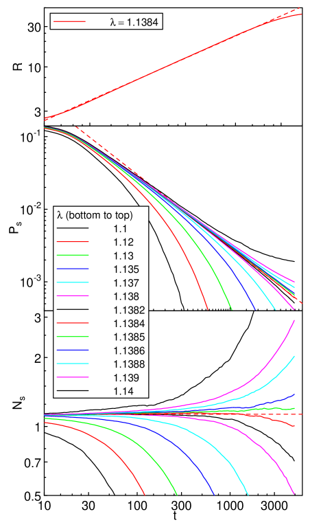
Figure 1: (Color online) Spreading simulations for the clean five-dimensional contact process: Radius $R$ of the active cloud, survival probability $P_{s}$ and number of active site $N_{s}$ vs. time $t$ for several infection rates $\lambda$ close to criticality. The system size is $70^{5}$ sites; the data are averages over $2\times 10^{5}$ to $6\times 10^{6}$ attempts, depending on $\lambda$. The dashed lines are fits of the data for $\lambda=1.1384$ to mean-field critical behavior, $R\sim t^{1/2}$, $P_{s}\sim t^{-1}$, and $N_{s}\sim t^{0}$.

From these data, we determine the clean critical infection rate to be $\lambda_{c}^{0}=1.13845(5)$ where the number in brackets is an estimate of the error of last digit. The survival probability $P_{s}$, the number of active sites $N_{s}$, and the radius of the active cloud $R$ at this infection rate can be fitted to the mean-field behavior $P_{s}\sim t^{-1}$, $N_{s}\sim t^{0}$, and $R\sim t^{1/2}$ discussed in Sec. II.2 with high precision. (In fact, unrestricted power-law fits give the exponents $\delta=0.99(2)$, $\Theta=-0.005(10)$, and $1/z=0.503(6)$, respectively.) The downward turn of $R(t)$ at the latest times is due to the fact that the diameter of the active cloud reaches the system size, limiting further growth. We have therefore restricted our fits to times before that downturn. In addition to the spreading simulations we have also performed density decay simulations on lattice with $50^{5}$ sites. They confirm the value of the critical infection rate as well as the mean-field behavior $\rho\sim t^{-1}$ of the density at criticality.

To test the predictions (6) and (19) for the decay rate $\epsilon$ (and life time $\tau$) of small systems on the active side of the nonequilibrium transition, we have performed density decay runs for systems with sizes between $4^{5}$ and $12^{5}$ sites for several $\lambda$ slightly above $\lambda_{c}^{0}$. Fits of the density $\rho(t)$ to the expected exponential long-time decay $\rho\sim\exp(-\epsilon t)$ yield the decay rates $\epsilon$. Figure 2 shows how $\epsilon$ depends on the system size.

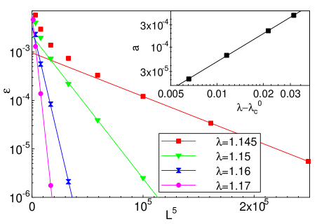
Figure 2: (Color online) Semilog. plot of the decay rate $\epsilon$ vs. system volume $L^{5}$ for several infection rates $\lambda$ slightly above the bulk critical rate $\lambda_{c}^{0}=1.13845$. The solid lines are fits to $\epsilon=\epsilon_{0}\exp(-aL_{RR}^{5})$. Inset: Decay coefficient $a$ vs. distance from bulk criticality $\lambda-\lambda_{c}^{0}$. The solid line is a power-law fit giving the exponent 1.99(3) and the prefactor $a^{\prime}=0.48(6)$.

After initial transients for very small systems , the data follow the exponential dependence $\epsilon=\epsilon_{0}\exp(-aL_{RR}^{5})$ predicted in eq. (6). The decay coefficient $a$ increases as $(\lambda-\lambda_{c}^{0})^{2}$ with increasing distance from criticality, as predicted in eq. (19).

Note that we have used periodic boundary conditions in the simulations leading to Fig. 2. In contrast, real rare regions embedded in a nearly critical bulk have complicated fluctuating boundary conditions that cannot be simulated easily without simulating the bulk system itself. However, the exponential dependence (6) of the life time on the rare region volume is a bulk effect and thus independent of the boundary conditions. Moreover the functional form of the finite-size scaling relation (19) does not change when changing the boundary conditions, only the prefactor $a^{\prime}$ does. The results in Fig. 2 thus confirm the predicted behavior but the value of $a^{\prime}$ resulting from the fit in the inset cannot be expected to be accurate; instead it provides an upper bound.

IV.3 Disordered five-dimensional contact process

We introduce quenched spatial disorder by making the infection rates $\lambda_{i}$ independent random variables drawn from the binary distribution (3). We parameterize the higher and lower of the two infection rates as $\lambda_{h}=\lambda$ and $\lambda_{l}=c\lambda$ where $c\leq 1$ is a fixed constant while $\lambda$ remains the tuning parameter of the transition. To explore the effects of weak and moderately strong disorder, we first set $c=0.1$ or 0.3 and vary the concentration $p$ of the higher rates from 0.8 to 0.2.

Figure 3 shows the results of density decay simulations (starting from a completely active lattice) for systems of $50^{5}$ sites with $p=0.2$ and $c=0.3$.

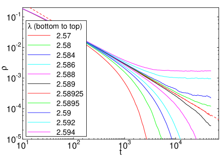
Figure 3: (Color online) Density of active sites $\rho$ vs. time $t$ for a disordered five-dimensional contact process with $p=0.2$ and $c=0.3$. The data are averages over 5 to 100 disorder configurations, depending on $\lambda$, each with $50^{5}$ lattice sites (one run per disorder configuration). The dashed line represents a power-law fit of the critical curve, $\lambda=2.58925(20)$, giving the exponent $\delta=0.99(2)$.

The time dependence of the density of active sites at the critical infection rate of $\lambda_{c}=2.58925$ follows the mean-field prediction $\rho\sim t^{-1}$ with high accuracy. We have performed analogous density decay simulations for two more parameter sets, $p=0.5,c=0.3$ and $p=0.8,c=0.1$. In both cases, we find the same mean-field decay $\rho\sim t^{-1}$ at criticality.

In addition to the density decay runs, we have also carried out spreading simulations on systems of $60^{5}$ sites for $p=0.5,c=0.3$. There resulting survival probability $P_{s}$, number of active sites $N_{s}$, and cloud radius $R$ are shown in Fig. 4.

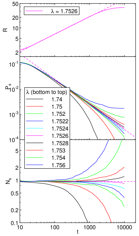
Figure 4: (Color online) Number of active sites $N_{s}$, survival probability $P_{s}$, and cloud radius $R$ vs. time $t$ for a disordered five-dimensional contact process with $p=0.5$ and $c=0.3$. The data are averages over 1000 to 10000 disorder configurations of $60^{5}$ sites (1000 trials per disorder configurations). The dashed lines are fits of the data for $\lambda=1.7526$ to mean-field critical behavior, $R\sim t^{1/2}$, $P_{s}\sim t^{-1}$, and $N_{s}\sim t^{0}$.

At criticality, $\lambda_{c}=1.7526$, the data follow the mean-field predictions $P_{s}\sim t^{-1}$ and $N_{s}\sim t^{0}$ with high accuracy. We thus conclude that the five-dimensional (weakly and moderately) disordered contact process features mean-field critical behavior, in agreement with the Harris criterion.

What about the power-law Griffiths singularities predicted in Sec. III? The simulations of the systems discussed so far [disorder parameters ($p=0.2,c=0.3$), ($p=0.5,c=0.3$), and ($p=0.8,c=0.1$)] do not show any trace of power-law behavior in the Griffiths region, i.e., for infection rates between the clean critical point $\lambda_{c}^{0}$ and the critical point $\lambda_{c}$ of the disordered system. Instead, the survival probability (for spreading simulations) and the density of active sites (for density decay runs) decay exponentially with time as would be expected in the absence of Griffiths singularities. We believe the reason why we cannot observe the Griffiths singularities is that their maximum dynamical exponent $z^{\prime}_{c}$ is too small (or, correspondingly, the Griffiths exponent $d/z^{\prime}$ is too large) in these moderately disordered systems . As a result, the Griffiths singularities dominate the bulk contribution only after very long times which are unreachable within our simulations.

To test this hypothesis, we have studied stronger disorder by setting $p=0.1$ and $c=0.1$. The concentration $p=0.1$ of strongly infecting sites (having $\lambda_{i}=\lambda_{h}=\lambda$) is below the site percolation threshold $p_{c}=0.1408$ Grassberger (2003). Establishing long-range order (activity) therefore relies on the weak sites with infection rates $\lambda_{i}=c\lambda$. As a result, the critical point $\lambda_{c}$ is much higher than the clean value $\lambda_{c}^{0}$. This, in turn, puts rare regions consisting of only strong sites ($\lambda_{i}=\lambda$) deep in the active phase, increasing their decay coefficient $a$ and with it the Griffiths dynamical exponent $z^{\prime}$ [see eq. (18)].

Figure 5 shows results of density decay simulation for systems of $51^{5}$ sites with $p=0.1$ and $c=0.1$.

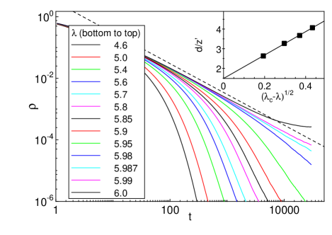
Figure 5: (Color online) Density of active sites $\rho$ vs. time $t$ for a disordered five-dimensional contact process with $p=0.1$ and $c=0.1$. The data are averages over 100 to 500 disorder configurations, depending on $\lambda$, each with $51^{5}$ lattice sites (one run per disorder configuration). The critical infection rate is $\lambda\approx 5.987$. The dashed line represents the mean field power-law with an arbitrary prefactor. The subcritical curves ($\lambda\leq 5.95$) show Griffiths singularities $\rho\sim t^{-d/z^{\prime}}$ rather than exponential decay. (The curve for $\lambda=5.98$ has not reached the asymptotic regime, yet.) Inset: Extrapolation of the Griffiths exponent $d/z^{\prime}$ for $\lambda=5.8\ldots 5.95$ to criticality (after Ref. Vojta and Hoyos (2014)).

The density decay at the critical infection rate $\lambda_{c}=5.987$ again follows mean-field behavior $\rho\sim t^{-1}$, in agreement with the Harris criterion. However, for infection rates slightly below $\lambda_{c}$, the time dependence of the density of active sites follows a non-universal power-law, in agreement with eqs. (16) and (18). The inset of this figure shows the values of the Griffiths exponent $d/z^{\prime}$ resulting from power-law fits of the subcritical $\rho(t)$. Extrapolating $d/z^{\prime}$ to criticality yields a nonzero finite value, (in agreement with the prediction of Sec. III.2.

We have observed analogous subcritical power laws in simulations of systems with parameters ($p=0.1,c=0.05$) and ($p=0.1,c=0.02$). This raises the interesting question of what happens to the transition if we further increase the disorder strength by using smaller and smaller values of $c$. As the strongly infecting sites do not percolate for $p=0.1$, the critical infection rate $\lambda_{c}$ diverges in the limit $c\to 0$. Close to criticality, rare regions consisting of only strong sites are thus deeper and deeper in the active phase, i.e., they have larger and larger decay parameters $a$. Beyond some threshold value of $a$, the rare region contribution (16) to the density will decay more slowly than the bulk mean-field decay $\rho\sim t^{-1}$. It is clear that the critical behavior of such a system must be different from mean-field behavior. We emphasize that this results does not violate the Harris criterion. The reason is that the Harris criterion only holds for sufficiently weak disorder as it based on the disorder scaling close to the clean fixed point. The strong-disorder behavior is beyond the scope of the Harris criterion. Exploring the novel critical behavior expected for sufficiently strong disorder by numerical means is very demanding because small values of $c$ lead to extremely slow dynamics. Our simulations of systems with $p=0.1$ and $c$ between 0.001 and 0.05 show indications of non-mean-field behavior. However, within the system sizes accessible to our simulations ($70^{5}$ sites), we have not been able to resolve the ultimate fate of these transitions.

V Conclusions

In summary, we have investigated the nonequilibrium phase transition of the five-dimensional contact process with quenched spatial disorder. This system is a prototypical example of a class of transitions that fulfill the Harris criterion, predicting clean critical behavior, but also feature strong power-law Griffiths singularities according to the rare region classification of Refs. Vojta (2006); Vojta and Schmalian (2005). To reconcile these predictions, we have adapted to absorbing state transitions an optimal fluctuation theory recently developed in the context of quantum phase transitions Vojta and Hoyos (2014). This optimal fluctuation theory considers the scaling of weak disorder close to the clean critical point and establishes a relation between the fate of the average disorder strength and the Griffiths singularities.

For clean critical points below the upper critical dimension $d_{c}^{+}$, both are controlled by the same inequality: If $d\nu_{\perp}<2$, weak disorder is relevant and destabilizes the clean critical behavior while the Griffiths dynamical exponent $z^{\prime}$ increases with the renormalized disorder strength upon approaching criticality. In contrast, if $d\nu_{\perp}>2$, the clean critical behavior is stable because weak disorder is irrelevant. At the same time, $z^{\prime}$ takes a nonzero finite value at the transition. It is small for weak disorder and increases with the disorder strength.

For clean critical points above the upper critical dimension $d_{c}^{+}$, the situation is more complex. Harris’ inequality $d\nu_{\perp}>2$ still governs the fate of the average disorder strength under coarse graining. However, the behavior of the Griffiths dynamical exponent $z^{\prime}$ is controlled by the value of $d_{c}^{+}$. If $d_{c}^{+}\nu_{\perp}<2$, the Griffiths dynamical exponent diverges, if $d_{c}^{+}\nu_{\perp}\geq 2$, it remains finite at the transition point.

The five-dimensional contact process falls into the latter class. Its clean critical point is above the upper critical dimension $d_{c}^{+}=4$. According to the Harris criterion $d\nu_{\perp}=5/2>2$, weak spatial disorder is irrelevant. Moreover as $d_{c}^{+}\nu=2$, our optimal fluctuation theory predicts the Griffiths dynamical exponent to remain finite at the transition. For sufficiently weak disorder, the Griffiths singularities thus provide a subleading correction to the mean-field behavior at criticality. Our Monte Carlo simulations have confirmed these predictions. We have indeed found mean-field critical behavior over a wide range of disorder strength. For the weakest disorder, we have not observed any Griffiths singularities. We attribute this to the fact that the Griffiths dynamical exponent remains very small in these cases, making the Griffiths singularities unobservable within accessible system sizes and simulation times. We have observed power-law Griffiths singularities for larger disorder. In agreement with the theoretical predictions, $z^{\prime}$ extrapolates to a finite value at criticality. For even larger disorder, our simulations show indications of a change in critical behavior because the Griffiths singularities become stronger than the mean-field critical singularities. We note that a similar coexistence of mean-field behavior and Griffiths singularities has also been observed in the contact process on networks Juhász et al. (2012).

It is instructive to relate the fate of $z^{\prime}$ at the bulk transition to the geometry of the rare regions. If $d\nu_{\perp}\geq 2$ (or, above the upper critical dimension, $d_{c}^{+}\nu_{\perp}\geq 2$), the most relevant rare regions are small compact clusters deep in the ordered phase. They effectively decouple from the bulk which explains why the Griffiths dynamical exponent $z^{\prime}$ is independent of the bulk exponent $z$. In contrast, for $d\nu_{\perp}<2$ (or $d_{c}^{+}\nu_{\perp}<2$ above the upper critical dimension), the relevant rare regions become larger and larger as the bulk transition is approached. At criticality they effectively become indistinguishable from the bulk. As the bulk $z$ is infinite, this explains why $z^{\prime}$ diverges at criticality.

Let us conclude by putting our results into the broader perspective of the rare region classification developed in in Refs. Vojta and Schmalian (2005); Vojta (2006). The optimal fluctuation theory developed in Ref. Vojta and Hoyos (2014) and generalized to absorbing state transitions in the present paper applies to class B of this classification. This class contains systems whose rare regions are right at the lower critical dimension, $d_{RR}=d_{c}^{-}$, leading to power-law Griffiths singularities. The results of the optimal fluctuation theory allow us to further subdivide class B. If $d\nu_{\perp}>2$ (below the upper critical dimension) or if both $d\nu_{\perp}>2$ and $d_{c}^{+}\nu_{\perp}\geq 2$ (above the upper critical dimension), the system is in class B1 in which clean critical behavior coexists with subleading Griffiths singularities. The five-dimensional contact process belongs to this subclass, as does the Ashkin-Teller quantum spin chain discussed in Ref. Vojta and Hoyos (2014) (for $\epsilon<-1/2$). In contrast, if at least one of the inequalities is violated, we expect the critical point to be modified by the disorder (class B2). In most explicit examples in this subclass such as the transverse-field Ising model Fisher (1992, 1995), itinerant quantum magnets Hoyos et al. (2007); Vojta et al. (2009b), or the contact process in $d<4$ Hooyberghs et al. (2003); Hoyos (2008); Vojta and Dickison (2005); de Oliveira and Ferreira (2008); Vojta et al. (2009a); Vojta (2012), the result is an infinite-randomness critical point, but other strong-disorder scenarios cannot be excluded.

A particularly interesting situation arises above the upper critical dimension if $d\nu_{\perp}>2$ but $d_{c}^{+}\nu_{\perp}<2$. The Harris criterion is fulfilled, but our theory suggests dominating Griffiths singularities because $z^{\prime}$ becomes large. This opens up the exciting possibility that non-perturbative rare region physics can modify the transition even if the Harris criterion is fulfilled. Interestingly, recent strong-disorder renormalization group calculations in $d>4$ Kovács and Iglói (2011) of the random transverse-field Ising model (for which $d_{c}^{+}\nu_{\perp}=3/2<2$) show infinite-randomness criticality even for infinite dimensions.

References

- Grinstein (1985) G. Grinstein, in Fundamental Problems in Statistical Mechanics VI, edited by E. G. D. Cohen (Elsevier, New York, 1985) p. 147.
- Vojta (2006) T. Vojta, J. Phys. A 39, R143 (2006).
- Vojta (2010) T. Vojta, J. Low Temp. Phys. 161, 299 (2010).
- Motrunich et al. (2000) O. Motrunich, S. C. Mau, D. A. Huse, and D. S. Fisher, Phys. Rev. B 61, 1160 (2000).
- Harris (1974a) A. B. Harris, J. Phys. C 7, 1671 (1974a).
- Griffiths (1969) R. B. Griffiths, Phys. Rev. Lett. 23, 17 (1969).
- McCoy (1969) B. M. McCoy, Phys. Rev. Lett. 23, 383 (1969).
- Vojta and Schmalian (2005) T. Vojta and J. Schmalian, Phys. Rev. B 72, 045438 (2005).
- Imry (1977) Y. Imry, Phys. Rev. B 15, 4448 (1977).
- Vojta (2003a) T. Vojta, Phys. Rev. Lett. 90, 107202 (2003a).
- Vojta (2003b) T. Vojta, J. Phys. A 36, 10921 (2003b).
- Thill and Huse (1995) M. Thill and D. A. Huse, Physica A 214, 321 (1995).
- Fisher (1995) D. S. Fisher, Phys. Rev. B 51, 6411 (1995).
- Young and Rieger (1996) A. P. Young and H. Rieger, Phys. Rev. B 53, 8486 (1996).
- Harris (1974b) T. E. Harris, Ann. Prob. 2, 969 (1974b).
- Hooyberghs et al. (2003) J. Hooyberghs, F. Iglói, and C. Vanderzande, Phys. Rev. Lett. 90, 100601 (2003).
- Vojta and Dickison (2005) T. Vojta and M. Dickison, Phys. Rev. E 72, 036126 (2005).
- de Oliveira and Ferreira (2008) M. M. de Oliveira and S. C. Ferreira, J. Stat. Mech. 2008, P11001 (2008).
- Vojta et al. (2009a) T. Vojta, A. Farquhar, and J. Mast, Phys. Rev. E 79, 011111 (2009a).
- Vojta (2012) T. Vojta, Phys. Rev. E 86, 051137 (2012).
- Vojta and Hoyos (2014) T. Vojta and J. A. Hoyos, Phys. Rev. Lett. 112, 075702 (2014).
- Grassberger and de la Torre (1979) P. Grassberger and A. de la Torre, Ann. Phys. (NY) 122, 373 (1979).
- Janssen (1981) H. K. Janssen, Z. Phys. B 42, 151 (1981).
- Grassberger (1982) P. Grassberger, Z. Phys. B 47, 365 (1982).
- Marro and Dickman (1999) J. Marro and R. Dickman, Nonequilibrium Phase Transitions in Lattice Models (Cambridge University Press, Cambridge, 1999).
- Lübeck (2004) S. Lübeck, Int. J. Mod. Phys. B 18, 3977 (2004).
- Hinrichsen (2000) H. Hinrichsen, Adv. Phys. 49, 815 (2000).
- Jensen (1999) I. Jensen, J. Phys. A 32, 5233 (1999).
- Voigt and Ziff (1997) C. A. Voigt and R. M. Ziff, Phys. Rev. E 56, R6241 (1997).
- Noest (1986) A. J. Noest, Phys. Rev. Lett. 57, 90 (1986).
- Noest (1988) A. J. Noest, Phys. Rev. B 38, 2715 (1988).
- Barber (1983) M. N. Barber, in Phase Transitions and Critical Phenomena, Vol. 8, edited by C. Domb and J. L. Lebowitz (Academic, New York, 1983) pp. 145–266.
- Cardy (1996) J. Cardy, Scaling and renormalization in statistical physics (Cambridge University Press, Cambridge, 1996).
- Hoyos (2008) J. A. Hoyos, Phys. Rev. E 78, 032101 (2008).
- Brezin (1982) E. Brezin, J. Phys. (France) 43, 15 (1982).
- Kenna and Lang (1991) R. Kenna and C. B. Lang, Phys. Lett. B 264, 396 (1991).
- Berche et al. (2012) B. Berche, R. Kenna, and J.-C. Walter, Nucl. Phys. B 865, 115 (2012).
- Note (1) Originally, -scaling was thought to apply to periodic boundary conditions only, and not to the open boundary conditions more relevant for our rare regions. However, recent work Berche et al. (2012) shows that -scaling also holds for open boundary conditions.
- Lübeck and Janssen (2005) S. Lübeck and H.-K. Janssen, Phys. Rev. E 72, 016119 (2005).
- Janssen et al. (2007) H.-K. Janssen, S. Lübeck, and O. Stenull, Phys. Rev. E 76, 041126 (2007).
- Dickman (1999) R. Dickman, Phys. Rev. E 60, R2441 (1999).
- Note (2) These transients are due to the crossover from the critical regime for small to the active phase for larger .
- Note (3) In principle, one can estimate the value of the Griffiths exponent from eq. (18). However this requires knowing the coefficient for rare regions of arbitrary shape and, importantly, fluctuating boundary conditions reflecting a nearly critical bulk. As explained at the end of Sec. IV.2, this value is very hard to obtain.
- Grassberger (2003) P. Grassberger, Phys. Rev. E 67, 036101 (2003).
- Juhász et al. (2012) R. Juhász, G. Ódor, C. Castellano, and M. A. Muñoz, Phys. Rev. E 85, 066125 (2012).
- Fisher (1992) D. S. Fisher, Phys. Rev. Lett. 69, 534 (1992).
- Hoyos et al. (2007) J. A. Hoyos, C. Kotabage, and T. Vojta, Phys. Rev. Lett. 99, 230601 (2007).
- Vojta et al. (2009b) T. Vojta, C. Kotabage, and J. A. Hoyos, Phys. Rev. B 79, 024401 (2009b).
- Kovács and Iglói (2011) I. A. Kovács and F. Iglói, Phys. Rev. B 83, 174207 (2011).