Accuracy and transferability of GAP models for tungsten

Abstract

We introduce interatomic potentials for tungsten in the bcc crystal phase and its defects within the Gaussian Approximation Potential (GAP) framework, fitted to a database of first principles density functional theory (DFT) calculations. We investigate the performance of a sequence of models based on databases of increasing coverage in configuration space and showcase our strategy of choosing representative small unit cells to train models that predict properties only observable using thousands of atoms. The most comprehensive model is then used to calculate properties of the screw dislocation, including its structure, the Peierls barrier and the energetics of the vacancy-dislocation interaction. All software and raw data are available at www.libatoms.org.

Tungsten is a hard, refractory metal with the highest melting point (3695 K) among metals, and its alloys are utilised in numerous technological applications. The details of the atomistic processes behind the plastic behaviour of tungsten have been investigated for a long time and many interatomic potentials exist in the literature reflecting an evolution, over the past three decades, in their level of sophistication, starting with the Finnis-Sinclair (FS) potential Finnis and Sinclair (1984), embedded atom model (EAM) Daw and Baskes (1984), various other FS/EAM parametrisations Ackland and Thetford (1987); Sutton and Chen (1990); Wang et al. (2014); Ercolessi and Adams (1994), modified embedded atom models (MEAM) Baskes (1992); Wang and Boercker (1995); Lee et al. (2001); Marinica et al. (2013) and bond order potentials (BOP) Mrovec et al. (2007); Ahlgren et al. (2010); Li et al. (2011). While some of these methods have been used to study other transition metals Moriarty (1988); Xu and Moriarty (1996); Mrovec et al. (2004), there is renewed interest in modelling tungsten due to its many high temperature applications—e.g. it is one of the candidate materials for plasma facing components in the JET and ITER fusion projects Matthews et al. (2007); Neu et al. (2007); Pitts et al. (2013).

A recurring problem with empirical potentials, due to the use of fixed functional forms with only a few adjustable parameters, is the lack of flexibility: when fitted to reproduce a given property, predictions for other properties can have large errors. Figure 1 shows the basic performance of BOP and MEAM, two of the more sophisticated potentials that reproduce the correct screw dislocation core structure, and also the simpler FS, all in comparison with density functional theory (DFT). While the figure emphasises fractional accuracy, we show the corresponding absolute numerical values in Table 1. BOP is poor in describing the vacancy but is better at surfaces, whereas MEAM is the other way around. While this compromise can sometimes be made with good judgement for specific applications, many interesting properties, particularly those that determine the material behaviour at larger length scales, arise from the competition between different atomic scale processes, which therefore all need to be described equally well. For example, dislocation pinning, depinning and climb involve both elastic properties, core structure, as well as the interaction of dislocations with defects. One way to deal with this problem is to use multiple levels of accuracy as in QM/MM Bernstein et al. (2009) or to allow the parameters of the potential to vary in time and space Vita and Car (1997).

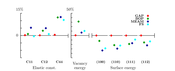
Figure 1: Fractional error in elastic constants and defect energies calculated with various interatomic potentials, as compared to the target DFT values.

	DFT	GAP	BOP	MEAM	FS
C11 [GPa]	517	518	522	544	514
C12 [GPa]	198	198	205	208	200
C44 [GPa]	142	143	160	160	157
vacancy energy [eV]	3.27	3.29	4.30	3.49	3.61
100 surface [eV/Å2]	0.251	0.252	0.221	0.167	0.179
110 surface [eV/Å2]	0.204	0.204	0.160	0.144	0.158
111 surface [eV/Å2]	0.222	0.222	0.180	0.184	0.202
112 surface [eV/Å2]	0.216	0.216	0.182	0.168	0.187

Table 1: Elastic constants and defect energies calculated with various interatomic potentials, and corresponding target DFT values.

Here we describe a milestone in a research programme aimed at creating a potential that circumvents the problem of fixed functional forms. The purpose of the present work is twofold. Firstly, we showcase the power of the non-parametric database driven approach by constructing an accurate potential and using it to compute atomic scale properties that are inaccessible to DFT due to computational expense. Secondly, while there has been vigorous activity recently in developing such models, most of the attention has been focussed on the interpolation method and the neighbourhood descriptors (e.g. neural networks Behler and Parrinello (2007); Behler et al. (2008); Artrith and Behler (2012), Shepherd interpolation Ischtwan and Collins (1994); Collins (2002), invariant polynomials Zhang et al. (2004); Huang et al. (2005); Xie et al. (2005), Gaussian processes Bartók et al. (2010, 2013, 2013); Gillan et al. (2013); Rupp et al. (2012)), rather less prominence was given to the question of how to construct suitable databases that ultimately determine the range of validity of the potential. Our second goal is therefore to study what kinds of configurations need to be in a database so that given material properties are well reproduced. A larger database costs more to create and the resulting potential is slower, but can be expected to be more widely applicable, thus providing a tuneable tradeoff between transferability, accuracy and computational cost.

In our Gaussian Approximation Potential (GAP) framework Bartók et al. (2010, 2013), the only uncontrolled approximation is the one essential to the idea of interatomic potentials: the total energy is written as a sum of atomic energies,

$$E=\sum_{i}\varepsilon(\mathbf{\hat{q}}_{i}),$$ (1)

with $\varepsilon$ a universal function of the atomic neighbourhood structure inside a finite cutoff radius as represented by the descriptor vector $\mathbf{\hat{q}}_{i}$ for atom $i$ (defined below). This function is fitted to a database of DFT calculations using Gaussian process regression MacKay (2003); Rasmussen and Williams (2006) so, in general, it is given by a linear combination of basis functions,

$$\varepsilon(\mathbf{\hat{q}}) =\sum_{j}\alpha_{j}K(\mathbf{\hat{q}}_{j},\mathbf{\hat{q}})\equiv\mathbf{k}(\mathbf{\hat{q}})^{T}\bm{\alpha},$$ (2)

where the sum over $j$ includes (some or all of) the configurations in the database, the vector of coefficients $\bm{\alpha}$ are given by linear algebra expressions (see below and in Bartók et al. (2010)), and the meaning of the covariance kernel $K$ is that of a similarity measure between different neighbour environments.

DFT code	CASTEP Clark et al. (2005) (version 6.01)
exchange-correlation functional	PBE
pseudopotential	ultrasoft (valence 5s2 5p6 5d4 6s2)
plane-wave energy cutoff	$600$ eV
maximum $k$-point spacing	$0.015$ $\text{\AA}^{-1}$
electronic smearing scheme	Gaussian
smearing width	$0.1$ eV
atomic environment kernel	SOAP
$f_{cut}(r)=\begin{cases}1&0<r\leq(r_{\text{cut}}-r_{\Delta})\\ \frac{1}{2}\cos(1+\pi\frac{r-r_{\text{cut}}+r_{\Delta}}{r_{\Delta}})&(r_{\text{cut}}-r_{\Delta})<r\leq r_{\text{cut}}\\ 0&r_{\text{cut}}<r\end{cases}$
$\begin{aligned} \phi_{n}(r)&=\exp[-(r-r_{\text{cut}}n/n_{\textrm{max}})^{2}/2\sigma^{2}_{\textrm{atom}}]\\ \\[-6.69998pt] S_{nn^{\prime}}&=\int_{0}^{r_{\textrm{cut}}}\!\!\!\!\!\!\!\!\!\!dr\,r^{2}\phi_{n}(r)\phi_{n^{\prime}}(r)\qquad\mathbf{S}=\mathbf{U}^{T}\mathbf{U}\\[-6.69998pt] \\[-6.69998pt] \\[-9.70001pt] g_{n}(r)&=\sum_{{n^{\prime}}}(\mathbf{U}^{-1})_{n{n^{\prime}}}\phi_{n^{\prime}}(r)\end{aligned}$
$r_{\text{cut}}$	$5.0$ Å
$r_{\Delta}$	$1.0$ Å
$\sigma_{\nu}^{\text{(energy)}}$	$0.0001$ eV/atom
$\sigma_{\nu}^{\text{(force)}}$	$0.01$ eV/Å
$\sigma_{\nu}^{\text{(virial)}}$	$0.01$ eV/atom
$\sigma_{w}$	$1.0$ eV
$\sigma_{\text{atom}}$	$0.5$ Å
$\xi$	$4$
$n_{\text{max}}$	$14$
$l_{\text{max}}$	$14$
GAP software version	df1c4d9

Table 2: DFT parameters used to generate training data and GAP model parameters.

The expression for the coefficients $\alpha_{j}$—normally simple in Gaussian process regression—is more complicated in our case because the quantum mechanical input data we can calculate is not a set of values of the atomic energy function that we are trying to fit. Rather, the total energy of a configuration is a sum of many atomic energy function values, and the forces and stresses, which are also available analytically through the Hellmann-Feynman theorem, are sums of partial derivatives of the atomic energy function. The detailed derivation of the formulas shown below is in Snelson and Ghahramani (2006); Bartók (2010); Szlachta (2013). Let us collect all the input data values (total energies, force and stress components) into the vector $\mathbf{y}$ with $D$ components in total and denote by $\mathbf{y}^{\prime}$ the $N$ unknown atomic energy values corresponding to all the atoms that appear in all the input configurations. We construct a linear operator $\mathbf{L}$ that describes the relationship between them through $\mathbf{y}=\mathbf{L}^{T}\mathbf{y}^{\prime}$. For data values that represent total energies, the corresponding rows of $\mathbf{L}$ have just 0s and 1s as their elements, but for forces and stresses, the entries are differential operators such as $\partial/\partial x_{i}$ corresponding to the force on atom $i$ with cartesian $x$ coordinate $x_{i}$. Writing $K_{ij}\equiv K(\mathbf{\hat{q}}_{i},\mathbf{\hat{q}}_{j})$ for the element of the covariance matrix $\mathbf{K}_{NN}$ corresponding to atoms $i$ and $j$, the covariance matrix of size $D\times D$ of the observed data is,

$$\mathbf{K}_{DD}=\mathbf{L}^{T}\mathbf{K}_{NN}\mathbf{L},$$ (3)

where the differential operators in $\mathbf{L}$ act on the covariance function $K$ that defines $\mathbf{K}_{NN}$. In our applications, $N$ can exceed a hundred thousand, and therefore working with $N\times N$ matrices would be computationally very expensive. Because many atomic environments in our dataset are highly similar to one another, it is plausible that many fewer than $N$ atoms could be chosen to efficiently represent the range of neighbour environments. We choose $M$ representative atoms from the full set of $N$ atoms that appear in all the input configurations (typically with $M\ll N$), and denote the square covariance matrix between the $M$ representative atoms by $\mathbf{K}_{MM}$ and the rectangular covariance matrix between the $M$ representative atoms and all the $N$ atoms by $\mathbf{K}_{MN}$ (with $\mathbf{K}_{NM}=\mathbf{K}_{MN}^{T}$). The expression for the vector of coefficients in equation 2 is then,

$$\bm{\alpha}=[\mathbf{K}_{MM}+\mathbf{K}_{MN}\mathbf{L}\mathbf{\Lambda}^{-1}\mathbf{L}^{T}\mathbf{K}_{NM}]^{-1}\mathbf{K}_{MN}\mathbf{L}\mathbf{\Lambda}^{-1}\mathbf{y},$$ (4)

with

$$\mathbf{\Lambda}=\sigma^{2}_{\nu}\mathbf{I},$$ (5)

where the parameter $\sigma_{\nu}$ represents the tolerance (or expected error) in fitting the input data. It could be a single constant, but in practice we found it essential to use different tolerance values corresponding to the different kinds of input data, so that the $\mathbf{\Lambda}$ matrix is still diagonal, but has different values corresponding to total energies, forces and stresses as they appear in the data vector $\mathbf{y}$. Although one might initially expect zero error in ab initio input data, this is not actually the case due to convergence parameters in the electronic structure calculation. A further source of error in the fit is the uncontrolled approximation of equation (1), i.e. writing the total energy as a sum of local atomic energies. The numerical values we use are shown in Table 2. They are based on convergence tests of the DFT calculation carried out on example configurations.

We note the following remarks about the expression in (4). The quantum mechanically not defined and therefore unknown atomic energies for the input configurations, $\mathbf{y}^{\prime}$, do not appear. The number of components in the coefficient vector ${\bm{\alpha}}$ is $M$, so the sum in equation (2) is over the $M$ representative configurations. The cost of calculating ${\bm{\alpha}}$ is dominated by operations which scale like $O(NM^{2})$, so it can be significantly reduced by choosing $M$ to be smaller and accepting a reduced accuracy of the fit. After the fit is made the coefficient vector ${\bm{\alpha}}$ stays fixed, and the evaluation of the potential is accomplished by the vector dot product in (2) with most of the work going towards computing the vector $\mathbf{k}$ for each new configuration, and thus scaling like $O(M)$. The $M$ representative atoms can be chosen randomly, but we found it beneficial to employ the k-means clustering algorithm to choose the representative configurations.

We now turn to the specification of the kernel function. We use the “smooth overlap of atomic positions” (SOAP) kernel Bartók et al. (2013),

$$K_{ij}=\sigma^{2}_{w}|\mathbf{\hat{q}}_{i}\cdot\mathbf{\hat{q}}_{j}|^{\xi}$$ (6)

where the exponent $\xi$ is a positive integer parameter whose role is to “sharpen” the selectivity of the similarity measure, and $\sigma_{w}$ is an overall scale factor. Note that for the special choice of $\xi=1$, the Gaussian process regression fit is equivalent to simple linear regression, and so potential energy expression in (2) simplifies to $\varepsilon(\mathbf{\hat{q}})=\left(\sigma_{w}^{2}\sum_{j}{\alpha}_{j}\mathbf{\hat{q}}_{j}\right)\cdot\mathbf{\hat{q}}$, in which the term in parentheses can be precomputed once and for all. Unfortunately we found that such a linear fit significantly limits the attainable accuracy of the potential.

	Database:		Computational cost [ms/atom]	Elastic constants [GPa]	Phonon spectrum [THz]	Vacancy formation [eV]	Surface energy [eV/Å2]	Dislocation structure [$\text{\r{A}}^{-1}$]	Dislocation-vacancy binding energy [eV]	Peierls barrier [eV/b]
GAP1 :	2000 $\times$ primitive unit cell with varying lattice vectors		24.70	0.623	0.583	2.855	0.1452	0.0008
GAP2 :	GAP1 +	60 $\times$ 128-atom unit cell	51.05	0.608	0.146	1.414	0.1522	0.0006
GAP3 :	GAP2 +	vacancy in: 400 $\times$ 53-atom unit cell, 20 $\times$ 127-atom unit cell	63.65	0.716	0.142	0.018	0.0941	0.0004
GAP4 :	GAP3 +	$(100)$, $(110)$, $(111)$, $(112)$ surfaces 180 $\times$ 12-atom unit cell $(110)$, $(112)$ gamma surfaces 6183 $\times$ 12-atom unit cell	86.99	0.581	0.138	0.005	0.0001	0.0002	-0.960	0.108
GAP5 :	GAP4 +	vacancy in: $(110)$, $(112)$ gamma surface 750 $\times$ 47-atom unit cell	93.86	0.865	0.126	0.011	0.0001	0.0002	-0.774	0.154
GAP6 :	GAP5 +	$\frac{1}{2}\langle 111\rangle$ dislocation quadrupole 100 $\times$ 135-atom unit cell	93.33	0.748	0.129	0.015	0.0001	0.0001	-0.794	0.112

Table 3: Summary of the databases for six GAP models, in order of increasing breadth in the types of configurations they contain, together with the performance of the corresponding potentials with respect to key properties. The colour of the cells indicates a subjective judgement of performance: unacceptable (red), usable (yellow), good (green). The first five properties can be checked against DFT directly and so we report errors, but calculation of the last two properties are in large systems, so we report the values, converged with system size. The configurations are collected using Boltzmann sampling, for more details on the databases leading to the models see the supplementary information.

		Database:
		1	2	3	4	5	6	Total $M$
GAP1		2000						2000
GAP2		814	3186					4000
GAP3		366	1378	4256				6000
GAP4		187	617	1890	6306			9000
GAP5		158	492	1604	5331	2415		10000
GAP6		140	450	1500	4874	2211	825	10000

Table 4: Number of representative atomic environments in each database of the six GAP models. The rows represent the successive GAP models and the columns represent the configuration types in the databases, grouped according to which GAP model first incorporated them. The allocations shown are based on k-means clustering. The rightmost column shows the total number of representative atoms in each GAP model ($M$).

The elements of the descriptor vector $\mathbf{\hat{q}}$ are constructed as follows. The environment of the $i$th atom is characterised by the atomic neighbourhood density, which we define as

$$\rho_{i}(\mathbf{r}) =\sum_{j}e^{-|\mathbf{r}-\mathbf{r}_{ij}|^{2}/2\sigma^{2}_{\textrm{atom}}}f_{\mathrm{cut}}(|\mathbf{r}_{ij}|)$$ (7)

$$=\sum_{n<n_{\textrm{max}}\atop{l<l_{\textrm{max}}\atop|m|\leq l}}c^{i}_{nlm}g_{n}(|\mathbf{r}|)Y_{lm}(\mathbf{\hat{r}})$$

where $\mathbf{r}_{ij}$ are the vectors pointing to the neighbouring atoms, $\sigma_{\textrm{atom}}$ is a parameter corresponding to the “size” of atoms, $f_{\textrm{cut}}$ is a smooth cutoff function with compact support, and the expansion on the second line uses spherical harmonics and a set of orthonormal radial basis functions, $g_{n}$, with $n$, $l$ and $m$ the usual integer indices. The elements of the descriptor vector $\mathbf{\hat{q}}$ are then,

$$\mathbf{q}_{i}=\left\{\sum_{m}(c^{i}_{nlm})^{*}c^{i}_{n^{\prime}lm}\right\}_{nn^{\prime}l},\quad\mathbf{\hat{q}}_{i} =\mathbf{q}_{i}/|\mathbf{q}_{i}|$$ (8)

Values for the all the parameters and other necessary formulas are given in Table 2. The orthonormal radial basis is obtained from a set of equispaced Gaussians by Cholesky factorisation of their overlap matrix.

The SOAP kernel is special because it is not only invariant with respect to relabelling of atoms and rotation of either neighbour environment, but it is also faithful in the sense that $K$ only takes the value of unity when the two neighbourhoods are identical. This is because it is directly proportional to the overlap of the atomic neighbourhood densities, integrated over all three dimensional rotations $\hat{R}$,

$$K_{ij}\propto\left|\int\!\!d\hat{R}\left|\int\!\!d\mathbf{r}\rho_{i}(\mathbf{r})\rho_{j}(\hat{R}\mathbf{r})\right|^{2}\right|^{\xi}.$$ (9)

The SOAP kernel is therefore also manifestly smooth and slowly varying in Cartesian space, just as we know the true Born-Oppenheimer potential energy surface to be, away from electronic energy level crossings and quantum phase transitions. The entire GAP framework, including the choice of descriptor and the kernel, is designed so that its parameters are easy to set and the final potential is not very sensitive to the exact values. Some are physically motivated and stem from either the properties of the quantum mechanical potential energy surface ($r_{\textrm{cut}}$, $\sigma_{w}$, $\sigma_{\textrm{atom}}$) or the input data (e.g. $\sigma_{\nu}$), while others are convergence parameters and are set by a tradeoff between accuracy and computational cost ($n_{\textrm{max}}$, $l_{\textrm{max}}$, $M$). We include in the supplementary information a table demonstrating convergence of the fitted potential as a function of $n_{\textrm{max}}$, $l_{\textrm{max}}$, and $r_{\textrm{cut}}$. By far the most “arbitrary” part of the potential is thus the set of configurations chosen to comprise the training database.

Since the potential interpolates the atomic energy in the space of neighbour environments, we need good coverage of relevant environments in the database. We therefore need to start by deciding what material properties we wish to study and what are the corresponding neighbour environments. Our strategy is to define, for each material property, a set of representative small unit cell configurations that are amenable to accurate first principles calculation. In Table 3 we show the performance with respect to key material properties of six models, each fitted to a database that contains the configurations indicated on the left, in addition to all the configurations of the preceding one. In particular, as proposed by Vitek Vitek and Kroupa (1969); Vitek et al. (1970); Vitek (2004), the structure of $\frac{1}{2}\langle 111\rangle$ screw dislocations in bcc transition metals can be rationalised in terms of the strictly planar gamma surface concept, and therefore we use gamma surfaces in the database to ensure the coverage of neighbour environments found near the dislocation core. Where the dislocation structure is very far from correct, the numerical performance metric on it has been omitted. The table shows that, broadly speaking, the small representative unit cells are necessary and also sufficient to obtain each property accurately, so the GAP model interpolates well but does not extrapolate to completely new kinds of configurations. Adding new configurations never compromises the accuracy of previously incorporated properties. For information, Table 4 shows the results of the automatic allocation of the representative atoms in each GAP model to the various types of configurations.

We also show the performance of the final GAP₆ model on Figure 1 and omit the subscript from now. The phonon spectrum of the GAP model is shown in Figure 2 along with that of the DFT and FS. There is clear improvement with respect to the analytical model, but remaining deficiencies are also apparent. Strategies to enhance the training database in order to improve the description of phonons is an important future direction of study.

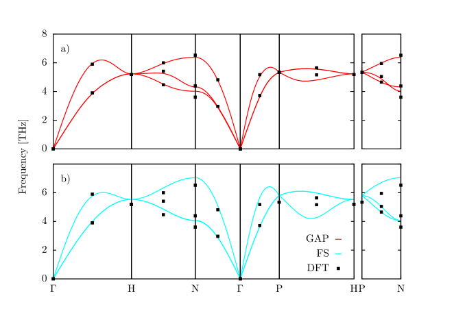
Figure 2: Phonon spectrum of bcc tungsten calculated using GAP and FS potentials, and some reference DFT values.

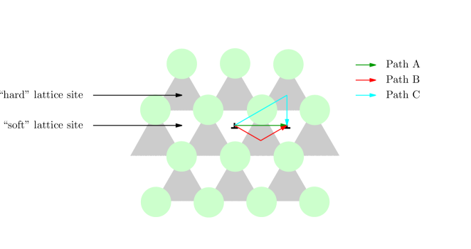
Figure 3: Representation of the three different initial transition paths for the Peierls barrier calculation. Path A corresponds to the linear interpolation directly from the initial to the final state, whereas paths B and C are the two distinct linear interpolations that include a potential meta-stable state (corresponding to the “hard” structure of the dislocation core) at reaction coordinate $r=0.5$.

We now investigate the properties of the $\frac{1}{2}\langle 111\rangle$ screw dislocation further by calculating the Peierls barrier using a transition state searching implementation of the string method E et al. (2002, 2007). Three different initial transition paths, shown in Figure 3, are used to explore the existence of the metastable state corresponding to a “hard” core structure Xu and Moriarty (1996); Ismail-Beigi and Arias (2000); Segall et al. (2003); Cereceda et al. (2013). We find that the “hard” core is not even locally stable in tungsten—starting geometry optimisation from there results in the dislocation line migrating to a neighbouring lattice site, corresponding to the “soft” core configuration. All three initial transition paths converge to the same minimum energy pathway (MEP), shown in Figure 4, with no “hard” core transition state. For large enough systems, the MEP is independent of the boundary conditions: the “quadrupole” calculations contained two oppositely directed dislocations in periodic boundary conditions, while the “cylinder” configurations had a single dislocation with fixed far field boundary conditions. For comparison we also plot the MEP of the Finnis-Sinclair model, and show the corresponding core structures using Nye tensor maps Hartley and Mishin (2005); Mendis et al. (2006). For the smallest periodic 135 atom model, we computed the energies at five points along the MEP using DFT to verify that the GAP model is indeed accurate for these configurations.

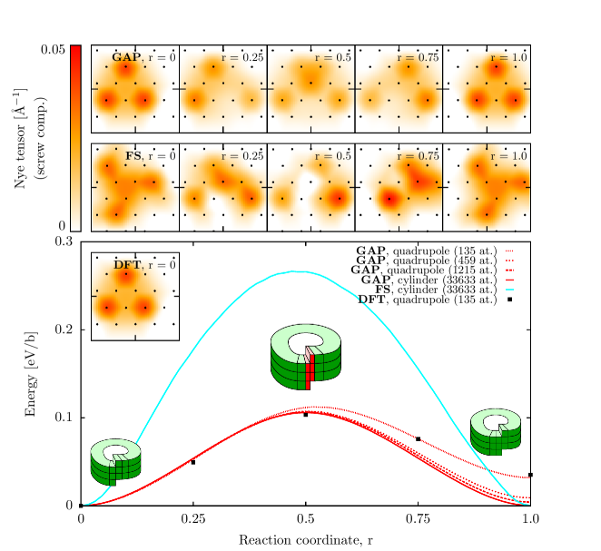
Figure 4: Top: the structure of the screw dislocation along the minimum energy path as it glides; bottom: Peierls barrier evaluated using GAP and FS potentials, along with single point checks with DFT in the 135 atom quadrupole arrangement.

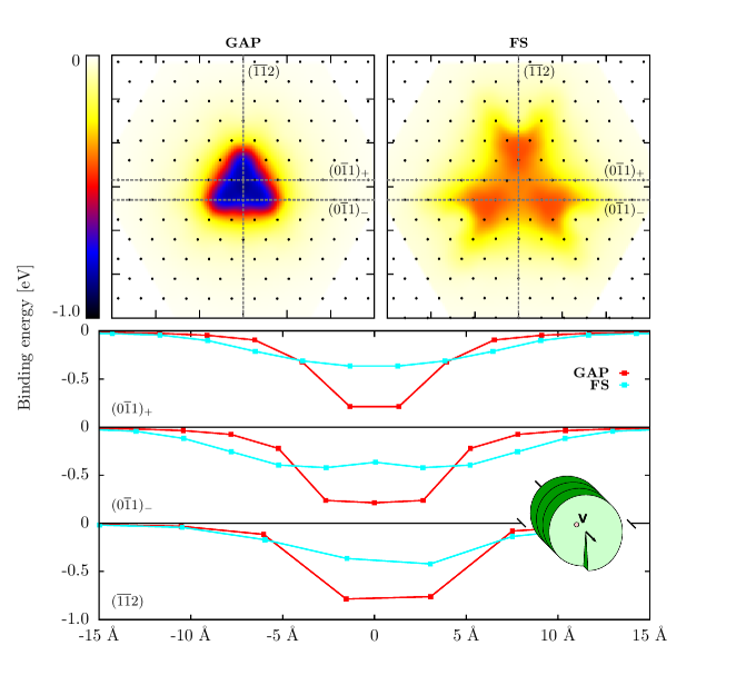
Figure 5: Dislocation-vacancy binding energy evaluated using GAP and FS potentials. The top panels show the interpolated binding energy using a heat map, the graphs below are slices of the same along the dotted lines shown in the top panels.

Due to the intrinsic smoothness of the potential, it can be expected to perform well for configurations which contain multiple defect structures as long as the local deformation around each defect with respect to the corresponding configurations in the database is small. So we finally turn to an example of the kinds of atomistic properties that are needed to make the connection to materials modelling on higher length scales, but are inaccessible to direct DFT calculations due to system size limitations imposed by the associated computational cost. Figure 5 shows the energy of a vacancy in the vicinity of a screw dislocation calculated in a system of over 100,000 atoms using cylindrical fixed boundary conditions 230 Å away from the core and with periodic boundary conditions applied along the dislocation line with a periodicity corresponding to three Burgers vectors. The Finnis-Sinclair potential underestimates this interaction by a factor of two.

Although the potential developed in this work does not yet constitute a comprehensive description of tungsten under all conditions, we have shown that the strategy of building a database of representative small unit cell configurations is viable, and will be continued with the incorporation of other crystal phases, edge dislocations, interstitials, etc. In addition to developing ever-more comprehensive databases and computing specific atomic scale properties with first principles accuracy on which higher length scale models can be built, our long term goal is to discover whether, in the context of a given material, an all-encompassing database could be assembled that contains a sufficient variety of neighbour environments to be valid for any configuration encountered under conditions of physically realistic temperatures and pressures. If that turns out to be possible, it would herald a truly new era of precision for atomistic simulations in materials science.