Area Coverage Under Low Sensor Density

Abstract

This paper presents a solution to the problem of monitoring a region of interest (RoI) using a set of nodes that is not sufficient to achieve the required degree of monitoring coverage. In particular, sensing coverage of wireless sensor networks (WSNs) is a crucial issue in projects due to failure of sensors. The lack of sensor equipment resources hinders the traditional method of using mobile robots to move around the RoI to collect readings. Instead, our solution employs supervised neural networks to produce the values of the uncovered locations by extracting the non-linear relation among randomly deployed sensor nodes throughout the area. Moreover, we apply a hybrid backpropagation method to accelerate the learning convergence speed to a local minimum solution. We use a real-world data set from meteorological deployment for experimental validation and analysis.

I Introduction

We are interested in the problem of monitoring a region of interest (RoI) with a limited set of nodes. In particular, this mainly occurs when the available sensors are not enough to achieve the required level of deployment density, e.g., coverage holes result due to temporary node failure. Traditionally, this problem is tackled using mobile robots that move through the uncovered points of the RoI, e.g., [1, 2, 3, 4]. However, such mobile solutions are not practical in many scenarios and suffer from many constraints. Firstly, the mobile node may not be able to move through the area, e.g., difficulty of the terrain’s obstacles or due to human activities. Secondly, as mobile nodes move among the designed locations, the system cannot provide the readings for all locations at all time instances. Thirdly, the mobile node suffers from the energy limitation. Fourthly, the development and deployment of a mobile node can be too costly.

Related solutions exploit the spatio-temporal correlation among sensor nodes to enhance area coverage and monitoring, e.g., [5, 6, 7]. These solutions are utilized to allocate the best locations to monitor the RoI using the available nodes. In particular, the RoI is divided into sensing zones and each zone is covered by one or more sensor nodes while maintaining the connectivity with other nodes, i.e., they exploit the joint coverage and connectivity problem. In contrast, we study the case in which the system suffers from severe scarcity of deployed nodes such that the sensing zone are not fully covered, i.e., some zones are not covered by any node. As a result, the solution extracts non-linear relations among zones to predict the value of the uncovered zones.

Neural networks mimic the human brain to find non-linear patterns in data. A supervised neural network consists of an input layer, one or more hidden layers, and an output layer. Layers are connected to each other using synapse weights. The backpropagation algorithm [8] provides a mechanism to fit the weights of the neural networks. In other words, the algorithm updates network weights to determine the connection between the input and the output data. This includes two main phases: propagation and weight tuning phase. Initially, the propagation phase spreads the input data forward through the network to generate the estimated output. Then, the estimated and the actual outputs are used to calculate the error value that is moved back through the network, i.e., from the output layer through the hidden layers to the input layer. Therefore, the neural network regulates itself to minimize the difference between the actual and the predicted vectors. Resilient propagation (Rprop) [9] is a backpropagation variant that tunes the supervised neural network’s weights by considering only the sign change of the neural network’s cost function. Another method adapts the use of the Broyden–Fletcher–Goldfarb–Shanno (BFGS) algorithm to train the neural network [10].

Our proposed algorithm is designed to predict readings from uncovered zones. Therefore, the algorithm increases the system coverage and support any random deployment while minimizing the operational costs. The system will be run in a centralized processing unit. Moreover, we show that the learning process (both execution time and performance) can be significantly enhanced by using Rprop for a few iterations and then BFGS for final tuning. In particular, Rprop converges faster than BFGS at initial iterations and with a lower computational complexity. However, BFGS outperforms Rprop in finding more accurate local minimum.

II Proposed algorithm

Suppose the scenario shown in Fig. 1. The points A to H represent the locations that the system must sense. However, the system designer has only a few sensor nodes, e.g., due to the limited funding, that are not sufficient to cover all monitored points. This shortage of nodes prevents achieving the required quality of service and results in coverage holes. The proposed solution works in the following procedure: The available sensor nodes are deployed at initial locations to cover part of the RoI, and the collected data is kept at the base station (throughout this paper, this data is called historical data). After some time (depending on the monitored phenomenon’s periodic behavior), some of the sensor nodes are moved to other points that are not already covered in the initial deployment (we call this as the moved subset). At the same time, a subset of the nodes are kept in their original locations (we call this as the fixed subset). This fixed subset is chosen by considering the area spatial correlation characteristic and the required monitoring accuracy, i.e., higher accuracy requires larger subset to be kept. Thereupon, the historical data is used to train a supervised neural network such that the input layer represents the fixed subset and the output layer is for the moved subset. Therefore, at any time instance and by using the fixed subset data, the uncovered locations (old locations of the moved subset) can be reproduced.

Suppose that the collected historical data $T$ consists of $n$ samples in the form $\mathbf{T}=\left\{\left(\mathbf{\vec{x}}^{(1)},\mathbf{\vec{y}}^{(1)}\right),...,\left(\mathbf{\vec{x}}^{(n)},\mathbf{\vec{y}}^{(n)}\right)\right\}$, where $\mathbf{\vec{x}}^{(i)}$ is the fixed subset data at time instance $i$ and $\mathbf{\vec{y}}^{(i)}$ is the moved subset data at the same instance. The predicted sensors’ output $\mathbf{\vec{p}}^{(i)}$ is generated when the input vector $\mathbf{\vec{x}}^{(i)}$ is placed at the neural network’s input neurons. The historical samples are used to train the neural network such as to minimize the sum of squares of the error (SSE) between the original output and the network predicted output as follows:

$$\text{SSE}=\sum_{j=1}^{n}\left\|\vec{\mathbf{y}}^{(j)}-\mathbf{\vec{p}}^{(j)}\right\|^{2}.$$

Choosing the number of neurons in the input and the output layer is a simple process. The input layer is formulated by a number of neurons that is identical to number of fixed nodes. Similarly, the output layer includes one neuron for each moved node. On the other hand, choosing the size of the hidden layer of a neural network is a key ingredient to achieve better estimation results. A widely accepted design method is to choose the size of the hidden layer to be between the sizes of the input and the output layers, i.e., to maintain the pyramid shape of the neural network. Moreover, using more than one hidden layer can efficiently enhance the neural network’s estimation ability. However, this increases the computation requirement of the learning process, i.e., algorithm’s execution time before convergence to local minimum.

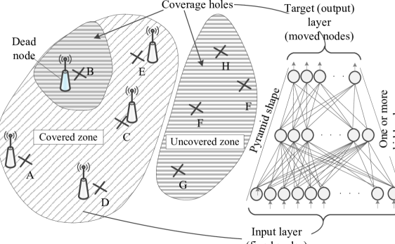
Figure 1: The problem of monitoring the RoI with a few sensor nodes along with a coverage hole due to a dead node.

Moreover, we propose a hybrid mechanism to accelerate the convergence of the backpropagation algorithm. Specifically, we noticed that the Rprop method outperforms the BFGS algorithm with fewer iterations. However, BFGS is more effective for minimizing the cost function over long runs. Then, it is important to realize that each iteration of BFGS requires the calculation of Hessian matrix. As a result, the BFGS method is more complex than Rprop in terms of computational requirement. A hybrid mechanism by starting the learning process using Rprop for a few iterations, e.g., one-tenth the total learning iterations, and then using BFGS for final tuning can significantly enhance the overall process in terms of average error and learning time.

III Results and evaluation

In this paper, we use a real data set from the Sensorscope project [11]. The data includes temperature readings from a meteorological application. The sensors (23 sensors) sense data in the range of -20 to 60 Celsius. To evaluate the proposed solution, we consider the test case that only 14 sensors are available and mark the rest as uncovered locations. Therefore, the 14 sensors are utilized to reproduce the data of the 23 sensors. Moreover, all the experiments in this paper use the cross-validation method [12] to test the solution efficiency. Accordingly, the historical data set is divided into five groups. The training is performed over four of them, while the remaining one is kept out for testing purposes. In this way, the testing is performed using data samples that are never seen by the generated model of the solution.

Figure 2 contains data series of a sensor node over time. Moreover, it includes estimated values assuming that the sensor was moved from its location. Even though the monitored area produces fluctuation pattern, the proposed method predicts reasonable estimations when that location was uncovered by physical sensors.

The performance of Rprop, BFGS, and the hybrid method is presented in Fig. 3. We use the sum of squares of error (SSE) to quantize the difference between the original and the estimated values. During an iteration of the learning process, the algorithm iterates over all learning samples to tune the neural network parameters. In Rprop, the weights are updated by multiplying the old value by a factor $\alpha$. In particular, if there is no sign change between successive iterations, the factor is set to be less than one, e.g., $\alpha=0.6$. Otherwise, it is set to be greater than one, e.g., $\alpha=1.2$. BFGS is a method that uses the Hessian matrix, i.e., a second order method, to find the optimization direction of unconstrained and nonlinear problems. BFGS converges to local minimum more accurately than the Rprop method. On the negative side, BFGS takes more time to converge than Rprop and requires more computational resources. Our hybrid method benefits from both algorithm capabilities by starting the learning process using Rprop, followed by BFGS at the second stage. This hybrid technique significantly facilitates the convergence process to the local minimum with a lower number of iterations.

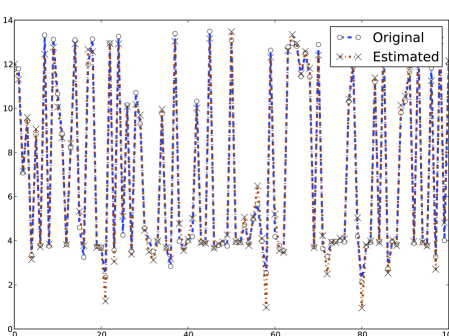
Figure 2: Performance analysis: Original readings and the algorithm estimation of them.

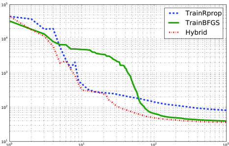
Figure 3: Comparison between the backpropagation methods: Rprop, BFGS, and the hybrid method.

For comparison purpose, the absolute error between the original and the predicted outputs is defined as follows:

$$\varepsilon_{abs}=\frac{1}{n}\sum_{j=1}^{n}\left|\mathbf{\vec{y}}^{(j)}-\mathbf{\vec{p}}^{(j)}\right|.$$

Accordingly, we compare the estimation capabilities of the algorithms with different number of hidden layers as summarized in Table I. Here, it is important to consider the tradeoff between the algorithm’s performance and the time required to learn the correlation among sensors (the more layers, the lower the average error, and the more time required to train the neural networks). However, if the network is not trained over sufficient iterations, the algorithm performance will degrade when using more layers, e.g., as in the case of using 5 layers instead of 4 layers with BFGS (Table I).

TABLE I: Comparison between the used neural network’s layers and methods over 1000 iterations. This includes the absolute error $(\varepsilon_{abs})$ in Celsius and the required learning time $\left(t_{learn}\right)$ in hours for each method. The learning time is just used to compare between the three algorithms.

# of layers and neurons at each layer	Rprop $(\varepsilon_{abs},t_{learn})$	BFGS $(\varepsilon_{abs},t_{learn})$	Hybrid $(\varepsilon_{abs},t_{learn})$
3 layers (14:11:9)	$(0.845,3.29)$	$(0.639,4.99)$	$(0.622,4.73)$
4 layers (14:13:12:9)	$(0.820,5.01)$	$(0.566,8.05)$	$(0.554,7.40)$
5 layers (14:13:12:11:9)	$(0.812,6.57)$	$(0.586,13.96)$	$(0.536,12.66)$

IV Summary and ongoing work

In this paper, we have proposed a solution to the problem of monitoring an area with a few number of sensor nodes. In particular, the method explores the spatial correlation among sensor nodes using supervised neural networks. Therefore, the proposed method predicts measurements at uncovered zones. Moreover, we have shown that a hybrid method of Rprop and BFGS can significantly enhance the learning stage in terms of performance and execution time.

In ongoing research, we aim to develop a model to select the number of Rprop and BFGS iterations in the hybrid method. Moreover, we will analyze the statistical models of the area which helps in selecting the moved and the static subsets of nodes, and we will connect this with the error control and bounding.

References

- [1] M. A. Batalin and G. S. Sukhatme, “Sensor coverage using mobile robots and stationary nodes,” in ITCom 2002: The Convergence of Information Technologies and Communications. International Society for Optics and Photonics, 2002, pp. 269–276.
- [2] C. Costanzo, V. Loscrí, E. Natalizio, and T. Razafindralambo, “Nodes self-deployment for coverage maximization in mobile robot networks using an evolving neural network,” Computer Communications, vol. 35, no. 9, pp. 1047–1055, 2012.
- [3] B. Liu, O. Dousse, P. Nain, and D. Towsley, “Dynamic coverage of mobile sensor networks,” IEEE Transactions on Parallel and Distributed Systems, vol. 24, no. 2, pp. 301–311, 2013.
- [4] M. Erdelj, V. Loscri, E. Natalizio, and T. Razafindralambo, “Multiple point of interest discovery and coverage with mobile wireless sensors,” Ad Hoc Networks, vol. 11, no. 8, pp. 2288–2300, 2013.
- [5] H. Gupta, V. Navda, S. Das, and V. Chowdhary, “Efficient gathering of correlated data in sensor networks,” ACM Transactions on Sensor Networks (TOSN), vol. 4, no. 1, p. 4, 2008.
- [6] M. Michaelides and C. G. Panayiotou, “Improved coverage in wsns by exploiting spatial correlation: the two sensor case,” EURASIP Journal on Advances in Signal Processing, vol. 2011, no. 1, pp. 1–11, 2011.
- [7] S. He, J. Chen, X. Li, X. Shen, and Y. Sun, “Leveraging prediction to improve the coverage of wireless sensor networks,” IEEE Transactions on Parallel and Distributed Systems, vol. 23, no. 4, pp. 701–712, 2012.
- [8] D. E. Rumelhart, G. E. Hinton, and R. J. Williams, Learning representations by back-propagating errors. MIT Press, Cambridge, MA, USA, 1988.
- [9] M. Riedmiller and H. Braun, “Rprop-a fast adaptive learning algorithm,” in Proceedings of the International Symposium on Computer and Information Science. Citeseer, 1992.
- [10] J. Ngiam, A. Coates, A. Lahiri, B. Prochnow, Q. V. Le, and A. Y. Ng, “On optimization methods for deep learning,” in Proceedings of the 28th International Conference on Machine Learning, 2011, pp. 265–272.
- [11] G. Barrenetxea, F. Ingelrest, G. Schaefer, and M. Vetterli, “Wireless sensor networks for environmental monitoring: the sensorscope experience,” in IEEE International Zurich Seminar on Communications. IEEE, 2008, pp. 98–101.
- [12] R. Kohavi, “A study of cross-validation and bootstrap for accuracy estimation and model selection,” in International Joint Conference on Artificial Intelligence, vol. 14, no. 2, 1995, pp. 1137–1145.