Anisotropic Landau-Lifshitz sigma models from $q$-deformed AdS${}_{5}\times$S⁵ superstrings

Abstract

We consider bosonic subsectors of the $q$-deformed AdS${}_{5}\times$S⁵ superstring action and study the classical integrable structure of anisotropic Landau-Lifshitz sigma models (LLSMs) derived by taking fast-moving string limits. The subsectors are 1) deformed AdS${}_{3}\,\times\,$S¹ and 2) R $\times$ deformed S³ . The cases 1) and 2) lead to a time-like warped $SL(2)$ LLSM and a squashed S³ LLSM, respectively. For each of them, we construct an infinite number of non-local conserved charges and show a quantum affine algebra at the classical level. Furthermore, a pp-wave like limit is applied for the case 1). The resulting system is a null-like warped $SL(2)$ LLSM and exhibits a couple of Yangians through non-local gauge transformations associated with Jordanian twists.

1 Introduction

The AdS/CFT correspondence M is a particular class of dualities between string (gravity) theories and gauge theories. It is firmly supported by an enormous amount of works to date and its various aspects have been elucidated. In particular, the discovery of an integrable structure behind it review is a triumph of modern theoretical and mathematical physics.

A significant feature of AdS/CFT is that the AdS${}_{5}\times$S⁵ background is represented by a supercoset

$$\mbox{AdS}_{5}\times\mbox{S}^{5}=\frac{PSU(2,2|4)}{SO(1,4)\times SO(5)}\,.$$ (1)

It enables us to construct the Green-Schwarz string action MT in terms of group elements and the string sigma model is classically integrable BPR . The supercoset (1) enjoys the $\mathbb{Z}_{4}$-grading that ensures the existence of an infinite number of conserved charges Luscher1 ; BIZZ ; Bernard-Yangian ; MacKay . Other possible cosets are classified from the consistency conditions for string backgrounds Zarembo-symmetric .

The next is to consider integrable deformations of AdS/CFT. There are two approaches to tackle this issue. The one is an algebraic approach based on $q$-deformations of the world-sheet S-matrix BK ; BGM ; HHM ; dLRT ; Arutyunov . The deformed S-matrices are constructed in a mathematically consistent way. The other is a geometric approach to argue deformations of target spaces of string sigma models. Integrable deformations of two-dimensional non-linear sigma models have a long history (For classic papers, see Cherednik ; FR ; BFP ). In the present, there is a renewed interest in this subject in relation to the study of AdS/CFT.

We will focus upon the latter approach here. Deformed target spaces are not represented by symmetric cosets, but typically by non-symmetric cosets (For arguments on some examples, see SYY ). A particularly simple and tractable example is squashed S³ and its integrable structure has been studied intensively KY ; KOY ; KYhybrid ; KY-Sch ; KMY-QAA ; exotic ; Jordanian-KMY ; ORU ; BR ; OU . In the recent, a generalization to higher dimensions has succeeded for arbitrary compact Lie groups and symmetric cosets DMV , by following the Yang-Baxter sigma model description Klimcik .

Just after that, a standard $q$-deformed AdS${}_{5}\times$S⁵ superstring action has been constructed with a linear R-operator of Drinfeld-Jimbo type Drinfeld1 ; Drinfeld2 ; Jimbo satisfying the modified classical Yang-Baxter equation DMV-string . Then the metric (in the string frame) and NS-NS two-form have been determined ABF . Some special cases of the background are examined in HRT and a mirror TBA is proposed in mirror .

On the other hand, there is another kind of $q$-deformations called Jordanian deformations R ; Jordanian ; KLM . Jordanian deformed AdS${}_{5}\times$S⁵ superstring actions have been constructed with linear R-operators satisfying classical Yang-Baxter equation KMY-JordanianAdSxS . A remarkable point is that partial deformations are possible in comparison to the standard $q$-deformation. In fact, as an example of deformation of AdS₅ , a complete type IIB supergravity solution has been found in KMY-JordanianIIB and it contains a three-dimensional Schrödinger spacetime (Sch₃) as a subspace. Furthermore, $\gamma$-deformed backgrounds LM ; Frolov and the gravity duals for non-commutative gauge theories HI ; MR ; DHH have been reproduced in MY1 and MY2 , respectively, in the context of the Yang-Baxter sigma model.

In this paper, we will concentrate on the standard $q$-deformation of the AdS${}_{5}\times$S⁵ superstring constructed in DMV-string . A serious problem is that the metric introduced in ABF is singular. In order to resolve the singularity, it would be a nice way to consider a non-relativistic limit of the string world-sheet. It is performed by considering fast-moving strings Kruczenski ; Rafael1 ; ST ; SL2 . For simplicity, we consider two subsectors, 1) deformed AdS${}_{3}\times$S¹ and 2) R$\times$ deformed S³ . The deformed AdS₃ is still singular and hence it is enough to take this subspace so as to argue how to avoid the singularity.

There is another advantage of taking a non-relativistic limit from the viewpoint of the classical integrable structure. While non-ultra local terms appear in the current algebra in the relativistic case, those do not appear in the non-relativistic case. Hence infinite-dimensional symmetries generated by conserved non-local charges can be studied in a definite manner without ambiguities.

This paper is organized as follows. Section 2 considers fast-moving string limits of the deformed AdS${}_{3}\times$S¹ and R$\times$deformed S³ subsectors of the standard $q$-deformed AdS${}_{5}\times$S⁵ . The resulting systems are a time-like warped $SL(2)$ LLSM and a squashed S³ LLSM, respectively. Section 3 reveals the classical integrable structure of the time-like warped $SL(2)$ LLSM. The Lax pair is constructed and a (classical analogue of) quantum affine algebra $U_{q}(\widehat{sl(2)})$ is presented. The classical $r$-matrix is of trigonometric type. In section 4 we study a pp-wave like limit of the time-like warped $SL(2)$ LLSM. Then the resulting system is a null-like warped $SL(2)$ LLSM. A direct computation leads to an exotic symmetry as in exotic and the classical $r$-matrix contains a deformation term. However, non-local gauge transformations can be performed by following Jordanian-KMY so as to undo Jordanian twists. As a result, a couple of Yangians ${\mathcal{Y}}(sl(2))$ are derived and the resulting $r$-matrix is of rational. Section 5 is devoted to conclusion and discussion.

In Appendix A, our convention of the $sl(2)$ and $su(2)$ generators are summarized. Appendix B explains the classical integrable structure of the squashed S³ LLSM. Also in this case, a quantum affine algebra $U_{q}(\widehat{su(2)})$ is exhibited. The classical $r$-matrix is of trigonometric type again. In Appendix C, we argue the relation between boundary conditions and conserved non-local charges. In Appendix D, a null-like warped LLSM is derived from a time-like LLSM via a pp-wave like limit. In Appendix E, we give the detailed computation of non-local gauge transformations in undoing Jordanian twists.

2 Fast-moving string limits of $q$-deformed AdS${}_{5}\times$S⁵

In this section, we first introduce the bosonic part of the $q$-deformed AdS${}_{5}\times$S⁵ superstring action constructed in DMV-string ; ABF . Then it is truncated to the following subsectors : 1) deformed AdS${}_{3}\times$S¹ and 2) R$\times$deformed S³ . By taking a fast-moving string limit, each of them leads to an anisotropic LLSM.

2.1 The $q$-deformed AdS${}_{5}\times$S⁵ background

The standard $q$-deformation of the AdS${}_{5}\times$S⁵ superstring has been constructed in DMV-string . Here we are interested in the bosonic part of the deformed action, where the metric (in the string frame) and NS-NS two-form have been determined in ABF .

The bosonic action is composed of the metric part $S_{G}$ and the Wess-Zumino (WZ) term $S_{\rm WZ}$ that describes the coupling to an NS-NS two-form as follows:

$$S = S_{G}+S_{\rm WZ}\,,$$ (2)

$$S_{G} = \int\!d\tau d\sigma\,\left[\,\mathcal{L}^{G}_{\rm AdS}+\mathcal{L}^{G}_{\rm S}\,\right]\,,\qquad S_{\rm WZ}=\int\!d\tau d\sigma\,\left[\,\mathcal{L}_{\textrm{AdS}}^{\rm WZ}+\mathcal{L}_{\textrm{S}}^{\rm WZ}\,\right]\,.$$

Here $S_{G}$ and $S_{\rm WZ}$ are divided into the AdS part and the internal sphere part.

The metric parts $\mathcal{L}_{\textrm{AdS}}^{G}$ and $\mathcal{L}_{\textrm{S}}^{G}$ are given by, respectively,

$$\mathcal{L}_{\textrm{AdS}}^{G} = -\frac{T_{(\varkappa)}}{2}\,\eta^{\mu\nu}\Bigl{[}-\dfrac{(1+\rho^{2})\,\partial_{\mu}t\partial_{\nu}t}{1-\varkappa^{2}\rho^{2}}+\dfrac{\partial_{\mu}\rho\partial_{\nu}\rho}{(1+\rho^{2})(1-\varkappa^{2}\rho^{2})}+\dfrac{\rho^{2}\,\partial_{\mu}\zeta\partial_{\nu}\zeta}{1+\varkappa^{2}\rho^{4}\sin^{2}\zeta}$$ (3)

$$\hskip 56.9055pt+\dfrac{\rho^{2}\cos^{2}\zeta\,\partial_{\mu}\psi_{1}\partial_{\nu}\psi_{1}}{1+\varkappa^{2}\rho^{4}\sin^{2}\zeta}+\rho^{2}\sin^{2}\zeta\,\partial_{\mu}\psi_{2}\partial_{\mu}\psi_{2}\Bigr{]}\,,$$

$$\!\!\mathcal{L}_{\textrm{S}}^{G} = -\frac{T_{(\varkappa)}}{2}\,\eta^{\mu\nu}\Bigl{[}\dfrac{(1-r^{2})\,\partial_{\mu}\phi\partial_{\nu}\phi}{1+\varkappa^{2}r^{2}}+\dfrac{\partial_{\mu}r\partial_{\mu}r}{(1-r^{2})(1+\varkappa^{2}r^{2})}+\dfrac{r^{2}\,\partial_{\mu}\xi\partial_{\nu}\xi}{1+\varkappa^{2}r^{4}\sin^{2}\xi}$$ (4)

$$\hskip 56.9055pt+\dfrac{r^{2}\cos^{2}\xi\,\partial_{\mu}\phi_{1}\partial_{\nu}\phi_{1}}{1+\varkappa^{2}r^{4}\sin^{2}\xi}+r^{2}\sin^{2}\xi\,\partial_{\mu}\phi_{2}\partial_{\nu}\phi_{2}\Bigr{]}\,.$$

Here the deformed AdS₅ part is parameterized by the coordinates $t\,,\psi_{1}\,,\psi_{2}\,,\zeta\,,\rho$ . The deformed S⁵ part is described by $\phi\,,\phi_{1}\,,\phi_{2}\,,\xi\,,r$ . The world-sheet metric $\eta_{\mu\nu}$ is taken as the flat metric $\eta_{\mu\nu}=(-1,+1)$ with the world-sheet coordinates $\sigma^{\mu}=(\sigma^{0},\sigma^{1})=(\tau,\sigma)$ . The periodic boundary condition is imposed for the $\sigma$-direction and the range is taken as $\sigma\in[0,2\pi]$ .

Then the deformation is measured by a real parameter $\varkappa\in[0,\infty)$ . This parameter can also be expressed in terms of another real parameter $\eta\in[0\,,1)$ like

$$\varkappa=\frac{2\eta}{1-\eta^{2}}\,.$$ (5)

When $\varkappa=0$ , the above action is reduced to the undeformed AdS${}_{5}\times$S⁵ one. The range of the coordinates is the same as that of the ones with $\varkappa=0$ . A $\varkappa$-dependent string tension $T_{(\varkappa)}$ is defined as

$$T_{(\varkappa)}\equiv T(1+\varkappa^{2})^{1/2}\,,\qquad T\equiv\dfrac{R^{2}}{2\pi\alpha^{\prime}}\,.$$ (6)

Here $T$ is a dimensionless string tension with $R^{2}$ , where $R$ is the AdS radius when $\varkappa=0$ .

Finally the WZ parts are given by, respectively,

$$\mathcal{L}_{\textrm{AdS}}^{WZ} = \frac{T_{(\varkappa)}}{2}\,\varkappa\,\epsilon^{\mu\nu}\dfrac{\rho^{4}\sin 2\zeta}{1+\varkappa^{2}\rho^{4}\sin^{2}\zeta}\,\partial_{\mu}\psi_{1}\partial_{\nu}\zeta\,,$$ (7)

$$\mathcal{L}_{\textrm{S}}^{WZ} = -\frac{T_{(\varkappa)}}{2}\,\varkappa\,\epsilon^{\mu\nu}\dfrac{r^{4}\sin 2\xi}{1+\varkappa^{2}r^{4}\sin^{2}\xi}\,\partial_{\mu}\phi_{1}\partial_{\nu}\xi\,,$$ (8)

where $\epsilon^{\mu\nu}$ is the totally anti-symmetric tensor on the string world-sheet and it is normalized as $\epsilon^{01}=+1$ . The WZ parts are proportional to $\kappa$ , and hence vanish when $\varkappa=0$ .

A deformed AdS${}_{3}\times$S³ subspace

For later purpose, we consider a deformed AdS${}_{3}\times$S³ subspace of the $q$-deformed AdS${}_{5}\times$S⁵ . By imposing the following conditions,

$$\zeta=0\,,\qquad\xi=0\,,$$ (9)

$S^{G}$ is restricted to a deformed AdS${}_{3}\times$S³ . The metric parts are given by

$$\mathcal{L}_{\textrm{AdS}_{3}}^{G} = -\frac{T_{(\varkappa)}}{2}\,\eta^{\mu\nu}\Bigl{[}-\dfrac{(1+\rho^{2})\,\partial_{\mu}t\partial_{\nu}t}{1-\varkappa^{2}\rho^{2}}+\dfrac{\partial_{\mu}\rho\partial_{\nu}\rho}{(1+\rho^{2})(1-\varkappa^{2}\rho^{2})}+\rho^{2}\,\partial_{\mu}\psi_{1}\partial_{\nu}\psi_{1}\Bigr{]}\,,$$ (10)

$$\mathcal{L}_{\textrm{S}^{3}}^{G} = -\frac{T_{(\varkappa)}}{2}\,\eta^{\mu\nu}\Bigl{[}\dfrac{(1-r^{2})\,\partial_{\mu}\phi\partial_{\nu}\phi}{1+\varkappa^{2}r^{2}}+\dfrac{\partial_{\mu}r\partial_{\mu}r}{(1-r^{2})(1+\varkappa^{2}r^{2})}+r^{2}\,\partial_{\mu}\phi_{1}\partial_{\nu}\phi_{1}\Bigr{]}\,.$$ (11)

Note that the $S_{\rm WZ}$ part vanishes under the condition (9).

To take fast-moving string limits, it is helpful to perform coordinate transformations,

$$\rho\rightarrow\sinh\rho\,,\qquad r\rightarrow\sin\theta\,.$$ (12)

Then the metric parts (10) and (11) are rewritten as

$$\mathcal{L}_{\textrm{AdS}_{3}}^{G} = -\frac{T_{(\varkappa)}}{2}\,\eta^{\mu\nu}\Bigl{[}-\dfrac{\cosh^{2}\rho\,\partial_{\mu}t\partial_{\nu}t}{1-\varkappa^{2}\sinh^{2}\rho}+\dfrac{\partial_{\mu}\rho\partial_{\nu}\rho}{1-\varkappa^{2}\sinh^{2}\rho}+\sinh^{2}\rho\,\partial_{\mu}\psi_{1}\partial_{\nu}\psi_{1}\Bigr{]}\,,$$ (13)

$$\mathcal{L}_{\textrm{S}^{3}}^{G} = -\frac{T_{(\varkappa)}}{2}\,\eta^{\mu\nu}\Bigl{[}\dfrac{\cos^{2}\theta\,\partial_{\mu}\phi\partial_{\nu}\phi}{1+\varkappa^{2}\sin^{2}\theta}+\dfrac{\partial_{\mu}\theta\partial_{\mu}\theta}{1+\varkappa^{2}\sin^{2}\theta}+\sin^{2}\theta\,\partial_{\mu}\phi_{1}\partial_{\nu}\phi_{1}\Bigr{]}\,.$$ (14)

This truncated action will be the starting point of our later arguments.

2.2 A fast-moving string limit of deformed AdS${}_{3}\times$S¹

Let us consider the string action on a deformed AdS${}_{3}\times$S¹ subsector of the truncated action. By setting that $\theta=0$ , the Lagrangian is given by

$$\mathcal{L}_{\textrm{AdS}_{3}\times\textrm{S}^{1}}^{G} = -\frac{T_{(\varkappa)}}{2}\,\eta^{\mu\nu}\Bigl{[}-\dfrac{\cosh^{2}\rho\,\partial_{\mu}t\partial_{\nu}t}{1-\varkappa^{2}\sinh^{2}\rho}+\dfrac{\partial_{\mu}\rho\partial_{\nu}\rho}{1-\varkappa^{2}\sinh^{2}\rho}$$ (15)

$$\hskip 85.35826pt+\sinh^{2}\rho\,\partial_{\mu}\psi_{1}\partial_{\nu}\psi_{1}+\partial_{\mu}\phi\partial_{\nu}\phi\Bigr{]}\,,$$

where an S¹ circle is described by $\phi$ .

To derive an LLSM from this subsector, let us perform a coordinate transformation,

$$\psi_{1}=\tilde{\psi}+t\,,\qquad\phi=\tilde{\phi}+t\,,\qquad\rho=\frac{\tilde{\rho}}{2}\,.$$ (16)

Then the Lagrangian (15) is rewritten as

$$\mathcal{L}_{\textrm{AdS}_{3}\times\textrm{S}^{1}}^{G} = -\frac{T_{(\varkappa)}}{2}\,\eta^{\mu\nu}\biggl{[}-\frac{\varkappa^{2}\sinh^{2}\frac{\tilde{\rho}}{2}\cosh^{2}\frac{\tilde{\rho}}{2}}{1-\varkappa^{2}\sinh^{2}\frac{\tilde{\rho}}{2}}\,\partial_{\mu}t\partial_{\nu}t+2\Bigl{(}\sinh^{2}\frac{\tilde{\rho}}{2}\partial_{\mu}\tilde{\psi}+\partial_{\mu}\tilde{\phi}\Bigr{)}\partial_{\nu}t$$ (17)

$$\hskip 56.9055pt+\frac{1}{4}\frac{\partial_{\mu}\tilde{\rho}\partial_{\nu}\tilde{\rho}}{1-\varkappa^{2}\sinh^{2}\frac{\tilde{\rho}}{2}}+\sinh^{2}\frac{\tilde{\rho}}{2}\partial_{\mu}\tilde{\psi}\partial_{\nu}\tilde{\psi}+\partial_{\mu}\tilde{\phi}\partial_{\nu}\tilde{\phi}\biggr{]}\,.$$

With the static gauge

$$t=\kappa\tau\,,$$

the following fast-moving string limit is taken,

$$\varkappa\rightarrow 0\,,\quad\dot{X}^{\mu}\rightarrow 0\,,\quad\kappa\rightarrow\infty\quad\textrm{with}\quad\kappa\varkappa,\quad\kappa\dot{X}^{\mu}:~{}~{}\textrm{fixed}\,.$$ (18)

Note that the above limit (18) contains a further condition on $\kappa\varkappa$ as well as the standard one discussed in Kruczenski ; ST ; SL2 .

After all, the resulting action is given by

$$S = \frac{T}{2}\int\!\!d\tau d\sigma\,\Bigl{[}-\frac{1}{4}\kappa^{2}\varkappa^{2}\sinh^{2}\tilde{\rho}+\kappa\bigl{[}(\cosh\tilde{\rho}-1)\dot{\tilde{\psi}}+2\dot{\tilde{\phi}}\bigr{]}$$ (19)

$$\hskip 56.9055pt-\frac{\acute{\tilde{\rho}}^{2}}{4}-\sinh^{2}\frac{\tilde{\rho}}{2}\,\acute{\tilde{\psi}}^{2}-\acute{\tilde{\phi}}^{2}\Bigr{]}\,.$$

Here $T_{(\varkappa)}$ has been reduced to the dimensionless tension $T$ after performing the limit (18) . A remarkable point is that the system (19) has no singular term in comparison to the original metric.

The Virasoro constraints are also rewritten under the limit (18). To the leading order in $\kappa$, the one of the Virasoro constraints becomes

$$0=\kappa\bigl{[}(\cosh\tilde{\rho}-1)\acute{\tilde{\psi}}+2\acute{\tilde{\phi}}\,\bigr{]}\,.$$ (20)

By eliminating $\acute{\tilde{\phi}}$ from (19) with (20), the leading-order action is given by

$$S = \frac{T}{2}\int\!\!d\tau d\sigma\,\Bigl{[}-\frac{1}{4}\kappa^{2}\varkappa^{2}\sinh^{2}\tilde{\rho}+\kappa\bigl{[}(\cosh\tilde{\rho}-1)\dot{\tilde{\psi}}+2\dot{\tilde{\phi}}\bigr{]}$$ (21)

$$\hskip 56.9055pt-\frac{1}{4}\bigl{(}\acute{\tilde{\rho}}^{2}+\sinh^{2}\tilde{\rho}\,\acute{\tilde{\psi}}^{2}\bigr{)}\Bigr{]}\,.$$

The above action is simple and contains just a single deformation term (only the first term).

A comparison to the time-like warped AdS₃ case

It is valuable to rewrite the action (21) by introducing new parameters,

$$C\equiv\frac{\varkappa^{2}}{4}\geq 0\,,\qquad L\equiv\dfrac{R^{2}\kappa}{2\pi\alpha^{\prime}}\,,\qquad\lambda\equiv\dfrac{R^{4}}{\alpha^{\prime 2}}\,.$$ (22)

Then the action (21) is rewritten as

$$S = \dfrac{L}{2}\!\int\!\!dtd\sigma\biggl{[}-C\cosh^{2}{\tilde{\rho}}+\bigl{[}(\cosh{\tilde{\rho}}-1)\partial_{t}\tilde{\psi}+2\partial_{t}\tilde{\phi}\bigr{]}$$ (23)

$$\hskip 56.9055pt-\dfrac{\lambda}{16\pi^{2}L^{2}}\bigl{[}(\partial_{\sigma}\tilde{\rho})^{2}+\sinh^{2}{\tilde{\rho}}\,(\partial_{\sigma}\tilde{\psi})^{2}\bigr{]}\biggr{]}\,.$$

Here $\tau$ is replaced by $t$ through $t=\kappa\tau$ . The deformation term has also been rewritten like $-C\sinh^{2}\tilde{\rho}\rightarrow-C\cosh^{2}\tilde{\rho}+C$ and then the constant term $C$ has been dropped off.

As a result, the derived action (23) agrees precisely with a fast-moving string limit of time-like warped AdS₃$\times$S¹ string sigma modelKameYoshi . Hence we call it time-like warped $SL(2)$ LLSM.

2.3 A fast-moving string limit of R$\times$deformed S³

We next consider the string action on an R$\times$deformed S³ subsector of the truncated action. By setting that $\rho=0$ , the Lagrangian is given by

$$\mathcal{L}_{\textrm{R}\times\textrm{S}^{3}}^{G}\!\!=-\frac{T_{(\varkappa)}}{2}\,\eta^{\mu\nu}\!\Bigl{[}-\partial_{\mu}t\partial_{\nu}t+\dfrac{\cos^{2}\theta\,\partial_{\mu}\phi\partial_{\nu}\phi}{1+\varkappa^{2}\sin^{2}\theta}+\dfrac{\partial_{\mu}\theta\partial_{\mu}\theta}{1+\varkappa^{2}\sin^{2}\theta}+\sin^{2}\theta\,\partial_{\mu}\phi_{1}\partial_{\nu}\phi_{1}\Bigr{]}\,.$$ (24)

Here the time coordinate in the AdS part is included as R. It should be remarked that the reduced system (24) is not singular due to the condition $\rho=0$ , even though the time direction has been included.

As in the previous subsection, let us first perform the coordinate transformation,

$$\phi=\varphi_{1}+\varphi_{2}\,,\qquad\phi_{1}=\varphi_{1}-\varphi_{2}\,,\qquad\varphi_{1}=t+\tilde{\varphi_{1}}\,.$$ (25)

Then the Lagrangian (24) is rewritten as

$$\mathcal{L}_{\textrm{R}\times\textrm{S}^{3}}^{G} = -\frac{T_{(\varkappa)}}{2}\,\eta^{\mu\nu}\biggl{[}-\frac{\varkappa^{2}\sin^{2}\theta\cos^{2}\theta}{1+\varkappa^{2}\sin^{2}\theta}\,\partial_{\mu}t\partial_{\nu}t+\Bigl{(}1-\frac{\varkappa^{2}\sin^{2}\theta}{1+\varkappa^{2}\sin^{2}\theta}\Bigr{)}\partial_{\mu}\theta\partial_{\nu}\theta$$ (26)

$$\hskip 14.22636pt+2\biggl{\{}\Bigl{(}1-\frac{\varkappa^{2}\sin^{2}\theta\cos^{2}\theta}{1+\varkappa^{2}\sin^{2}\theta}\Bigr{)}\,\partial_{\mu}\tilde{\varphi}_{1}+\Bigl{(}\cos 2\theta-\frac{\varkappa^{2}\sin^{2}\theta\cos^{2}\theta}{1+\varkappa^{2}\sin^{2}\theta}\Bigr{)}\,\partial_{\mu}\varphi_{2}\biggr{\}}\partial_{\nu}t$$

$$\hskip 42.67912pt+\Bigl{(}1-\frac{\varkappa^{2}\sin^{2}\theta\cos^{2}\theta}{1+\varkappa^{2}\sin^{2}\theta}\Bigr{)}(\partial_{\mu}\tilde{\varphi}_{1}\partial_{\nu}\tilde{\varphi}_{1}+\partial_{\mu}\varphi_{2}\partial_{\nu}\varphi_{2})$$

$$\hskip 71.13188pt+2\Bigl{(}\cos 2\theta-\frac{\varkappa^{2}\sin^{2}\theta\cos^{2}\theta}{1+\varkappa^{2}\sin^{2}\theta}\Bigr{)}\partial_{\mu}\tilde{\varphi}_{1}\partial_{\nu}\varphi_{2}\biggr{]}\,.$$

This Lagrangian is drastically simplified with the static gauge

$$t=\kappa\tau$$

and by taking the fast-moving string limit (18). The resulting action is

$$S = \frac{T}{2}\int\!\!d\tau d\sigma\,\Bigl{[}-\frac{1}{4}\kappa^{2}\varkappa^{2}\sin^{2}2\theta+2\kappa\bigl{[}\dot{\tilde{\varphi}}_{1}+\cos 2\theta\dot{\varphi}_{2}\bigr{]}$$ (27)

$$\hskip 65.44142pt-\acute{\theta}^{2}-\acute{\tilde{\varphi}}_{1}^{2}-\acute{\varphi}_{2}^{2}-2\cos 2\theta\,\acute{\tilde{\varphi}}_{1}\acute{\varphi}_{2}\Bigr{]}\,.$$

Here $T_{(\varkappa)}$ is replaced by $T$ after taking the limit (18) , again.

The Virasoro constraints are also changed under the limit (18). To the leading order in $\kappa$, the one of the Virasoro constraints is rewritten as

$$0=2\kappa[\acute{\tilde{\varphi}}_{1}+\cos 2\theta\acute{\varphi}_{2}]\,.$$ (28)

By eliminating $\acute{\tilde{\varphi}}_{1}$ from (27) with (28), the leading-order action is given by

$$S=\frac{T}{2}\int\!\!d\tau d\sigma\,\Bigl{[}-\frac{1}{4}\kappa^{2}\varkappa^{2}\sin^{2}2\theta+2\kappa\bigl{[}\dot{\tilde{\varphi}}_{1}+\cos 2\theta\dot{\varphi}_{2}\bigr{]}-\acute{\theta}^{2}-\sin^{2}2\theta\acute{\varphi}_{2}^{2}\Bigr{]}\,.$$ (29)

The resulting action is very simplified again.

A comparison to the squashed S³ case

It is worth rewriting the action (29) by introducing new variables,

$$\varphi_{2}=-\frac{1}{2}\tilde{\phi}\,,\qquad\theta=\frac{1}{2}\tilde{\theta}\,,$$ (30)

and new parameters

$$C\equiv\frac{\varkappa^{2}}{4}\geq 0\,,\qquad L\equiv\dfrac{R^{2}\kappa}{2\pi\alpha^{\prime}}\,,\qquad\lambda\equiv\dfrac{R^{4}}{\alpha^{\prime 2}}\,.$$ (31)

Then the action is rewritten as

$$S = \dfrac{L}{2}\int\!\!dtd\sigma\,\biggl{[}C\cos^{2}{\tilde{\theta}}-\bigl{[}\cos{\tilde{\theta}}\partial_{t}\tilde{\phi}-2\partial_{t}\tilde{\varphi}_{1}\bigr{]}$$ (32)

$$\hskip 71.13188pt-\dfrac{\lambda}{16\pi^{2}L^{2}}\bigl{[}(\partial_{\sigma}\tilde{\theta})^{2}+\sin^{2}{\tilde{\theta}}(\partial_{\sigma}\tilde{\phi})^{2}\bigr{]}\biggr{]}\,.$$

Here $\tau$ is replaced by $t$ through $t=\kappa\tau$ . The deformation term has been rewritten as $-C\sin^{2}\tilde{\theta}\rightarrow C\cos^{2}\tilde{\theta}-C$ and then the constant term $-C$ has been dropped off.

Finally, the resulting action (32) agrees exactly with a fast-moving string limit of R$\times$squashed S³ string sigma model Wen . Hence we refer to it as the squashed S³ LLSM.

3 Integrability of time-like warped $SL(2)$ LLSM

Let us argue the classical integrability of the time-like warped $SL(2)$ LLSM. The related infinite-dimensional symmetry is also discussed by explicitly constructing an infinite number of conserved non-local charges. In section 2 the periodic boundary condition has been imposed for the spatial direction of the string world-sheet. In the following sections, however, the string world-sheet is supposed to be spatially infinite in order to argue an infinite-dimensional symmetry based on non-local charges. In fact, the fast-moving string limit implies a decompactification limit of the $\sigma$-direction (For example, see the argument in 2.2 of AF ) . For the case of the squashed S³ LLSM, see Appendix B.

3.1 The classical action and Lax pair

The classical action of the time-like warped $SL(2)$ LLSM is given by

$$S = \frac{L}{2}\int^{\infty}_{-\infty}\!\!\!dtdx\,\biggl{[}-C\cosh^{2}\rho+\left(\cosh\rho-1\right)\partial_{t}\psi$$ (33)

$$\hskip 85.35826pt-\frac{\lambda}{16\pi^{2}L^{2}}\left[\left(\partial_{x}\rho\right)^{2}+\sinh^{2}\rho\left(\partial_{x}\psi\right)^{2}\right]\biggr{]}\,.$$

The world-sheet is a (1+1)-dimensional spacetime spanned by $t$ and $x$ and the spatial direction is infinite. The system is non-relativistic because the action contains the first order in time derivative and the second order in spatial derivative. The deformation parameter $C$ is restricted to $C\geq 0$ . When $C=0$ , an isotropic $SL(2)$ LLSM is reproduced.

It is convenient to introduce a vector representation $n^{a}$ ,

$$n^{0}=-\cosh\rho\,,\qquad n^{1}=\sinh\rho\sin\psi\,,\qquad n^{2}=\sinh\rho\cos\psi\,,$$ (34)

satisfying the following relation,

$$\left(n^{0}\right)^{2}-\left(n^{1}\right)^{2}-\left(n^{2}\right)^{2}=1\,.$$ (35)

Then the classical equations of motion are rewritten as

$$\partial_{t}n^{0}=\frac{\lambda}{8\pi^{2}L^{2}}\left(n^{1}\partial_{x}^{2}n^{2}-n^{2}\partial_{x}^{2}n^{1}\right)\,,$$

$$\partial_{t}n^{1}=\frac{\lambda}{8\pi^{2}L^{2}}\left(n^{0}\partial_{x}^{2}n^{2}-n^{2}\partial_{x}^{2}n^{0}\right)-2Cn^{0}n^{2}\,,$$

$$\partial_{t}n^{2}=\frac{\lambda}{8\pi^{2}L^{2}}\left(n^{1}\partial_{x}^{2}n^{0}-n^{0}\partial_{x}^{2}n^{1}\right)+2Cn^{0}n^{1}\,.$$ (36)

These are identical to the Landau-Lifshitz equations

$$\partial_{t}n_{a}=\varepsilon_{abc}n^{b}\left(\dfrac{\lambda}{8\pi^{2}L^{2}}\partial_{x}^{2}n^{c}+\mathcal{J}^{c}_{~{}d}n^{d}\right)\qquad(a=0,1,2)\,,$$ (37)

with an anisotropic matrix $\mathcal{J}$

$$\mathcal{J}^{a}_{~{}b}=\textrm{diag}(j+2C,j,j)\qquad(j:~{}\textrm{an~{}arbitrary~{}const.})\,.$$ (38)

Here we have introduced the totally anti-symmetric tensor $\varepsilon_{abc}$ with $\varepsilon_{012}=-1$. The $sl(2)$ indices are raised and lowered with $\gamma^{ab}=\textrm{diag}(-1\,,+1\,,+1)$ and its inverse, respectively.

Lax pair.

The Lax pair of the time-like warped $SL(2)$ LLSM is represented by FT

$$U(t,x;z) = \dfrac{i\alpha}{\sinh z}\left[-\cosh z\,n^{0}T^{0}+n^{1}T^{1}+n^{2}T^{2}\right]\,,$$ (39)

$$V(t,x;z) = \dfrac{i\beta}{\sinh z}\left[-\cosh z\left(n^{1}\partial_{x}n^{2}-n^{2}\partial_{x}n^{1}\right)T^{0}+\left(n^{0}\partial_{x}n^{2}-n^{2}\partial_{x}n^{0}\right)T^{1}\right.$$

$$\hskip 42.67912pt\left.+\left(n^{1}\partial_{x}n^{0}-n^{0}\partial_{x}n^{1}\right)T^{2}\right]$$

$$+\dfrac{\alpha\beta}{\sinh^{2}z}\left[-n^{0}T^{0}+\cosh z\,n^{1}T^{1}+\cosh z\,n^{2}T^{2}\right]\,,$$

with a spectral parameter $z\in\mathbb{C}$ and new parameters,

$$\alpha\equiv\dfrac{4\pi L}{\sqrt{\lambda}}\sqrt{C}\,,\qquad\beta\equiv\dfrac{\sqrt{\lambda}}{2\pi L}\sqrt{C}\,.$$ (40)

The equations of motion (36) are reproduced from the commutation relation,

$$\Bigl{[}\partial_{t}-V(t,x;z),\partial_{x}-U(t,x;z)\Bigr{]}=0\,.$$ (41)

Monodromy matrix.

The monodromy matrix is defined as

$$M(z)\equiv{\rm P}\exp\left[\int^{\infty}_{-\infty}\!\!\!dx~{}U(t,x;z)\right]\,,$$ (42)

where P denotes the path ordering. Due to the condition (41) , $M(z)$ is a conserved quantity,

$$\frac{d}{dt}M(z)=0\,.$$ (43)

Thus the expansion of $M(z)$ in terms of $z$ leads to an infinite number of conserved charges. The resulting algebra of the charges depends on the expansion point. For example, the expansions around $z=\pm\infty$ leads to a quantum affine algebra $U_{q}(\widehat{sl(2)})$ . We will elaborate a classical realization of it in the next subsection.

3.2 The standard $q$-deformation of $sl(2)$

We will show that a $q$-deformed $sl(2)$ is realized in the time-like warped $SL(2)$ LLSM.

While the $SL(2)$ symmetry is realized in an isotropic $SL(2)$ LLSM, it is broken to $U(1)$ due to the non-vanishing $C$ . The remaining $U(1)$ charge is given by

$$Q^{0}=-\dfrac{L}{2}\int^{\infty}_{-\infty}\!\!\!dx~{}n^{0}(x)\,.$$ (44)

Here it is worth noting that the broken components of $SL(2)$ , $1$ and $2$ are still realized as non-local symmetries even when $C\neq 0$ , as in the original system before taking the fast-moving string limit.

In order to show this fact, it is convenient to introduce $n^{\widehat{\pm}}$ defined as

$$n^{\widehat{\pm}}\equiv\frac{n^{1}\pm in^{2}}{\sqrt{2}}\,.$$ (45)

For the conservation of non-local charges, boundary conditions are sensitive. We take a rapidly damping condition so that $n^{\widehat{\pm}}$ vanish at the spatial infinities. This condition enables us to construct conserved non-local charges, as shown in Appendix C.

The conserved non-local charges are given by

$$Q^{\widehat{\pm}}=-\dfrac{L}{2}\int^{\infty}_{-\infty}\!\!\!dx~{}{\rm e}^{\alpha\chi(x)}n^{\widehat{\pm}}(x)\,,$$ (46)

where $\chi(x)$ is a non-local field defined as

$$\chi(x)\equiv\frac{1}{2}\int^{\infty}_{-\infty}\!\!\!dy~{}\epsilon(x-y)n^{0}(y)\,,$$ (47)

and $\epsilon(x)$ is the signature function defined as

$$\epsilon(x)\equiv\theta(x)-\theta(-x)$$ (48)

with the step function $\theta(x)$ . It is helpful to introduce the following relations:

$$\partial_{x}\chi=n^{0}\,,\qquad\partial_{t}\chi=i\frac{\lambda}{8\pi^{2}L^{2}}\left(n^{\widehat{+}}\partial_{x}n^{\widehat{-}}-n^{\widehat{-}}\partial_{x}n^{\widehat{+}}\right)\,.$$ (49)

Then the next is to compute the Poisson brackets of $Q^{0}$ and $Q^{\widehat{\pm}}$ . The Poisson brackets for $n^{a}\,(a=0,\widehat{\pm})$ are given by

$$\Big{\{}n^{a}(x),n^{b}(y)\Bigr{\}}_{\rm P}=-i\frac{2}{L}\,\varepsilon^{ab}_{~{}~{}c}n^{c}(x)\delta(x-y)\,.$$ (50)

Note that non-ultra local terms are not contained in comparison to the current algebra of principal chiral models.

With the brackets (50) , the brackets of $Q^{0}$ and $Q^{\widehat{\pm}}$ can be evaluated as

$$\Bigl{\{}Q^{\widehat{\pm}},Q^{0}\Bigr{\}}_{\rm P}=\pm iQ^{\widehat{\pm}}\,,$$ (51)

$$\Bigl{\{}Q^{\widehat{+}},Q^{\widehat{-}}\Bigr{\}}_{\rm P}=i\dfrac{L}{2\alpha}\sinh\Bigl{(}\dfrac{2\alpha}{L}Q^{0}\Bigr{)}\,.$$

This is a classical analogue of the standard $q$-deformation of $sl(2)$ Drinfeld2 ; Jimbo .

In addition, there exists another set of non-local conserved charges,

$$\widetilde{Q}^{\widehat{\pm}}=-\dfrac{L}{2}\int^{\infty}_{-\infty}\!\!\!dx~{}{\rm e}^{-\alpha\chi(x)}n^{\widehat{\pm}}(x)\,.$$ (52)

These can be obtained by changing the sign of $\alpha$ in $Q^{\widehat{\pm}}$ and hence $Q^{0}$ and $\widetilde{Q}^{\widehat{\pm}}$ also generate another $q$-deformed $sl(2)$ algebra,

$$\Bigl{\{}\widetilde{Q}^{\widehat{\pm}},{Q}^{0}\Bigr{\}}_{\rm P}=\pm i\widetilde{Q}^{\widehat{\pm}}\,,$$ (53)

$$\Bigl{\{}\widetilde{Q}^{\widehat{+}},\widetilde{Q}^{\widehat{-}}\Bigr{\}}_{\rm P}=i\dfrac{L}{2\alpha}\sinh\Bigl{(}\dfrac{2\alpha}{L}Q^{0}\Bigr{)}\,.$$

In subsection 3.4, we will show that a (classical analogue of) quantum affine algebra is generated by $Q^{0}$ , $Q^{\widehat{\pm}}$ and $\widetilde{Q}^{\widehat{\pm}}$ in the sense of Drinfeld’s first realization Drinfeld1 .

3.3 Monodromy expansions and higher non-local charges

An infinite number of conserved charges are obtained by expanding the monodromy matrix $M(z)$ with respect to a complex parameter $u=\textrm{e}^{-z}$ . Here we derive the conserved charges discussed in the previous subsection by expanding $M(z)$ . According to the expansion, other higher non-local charges are also obtained.

Depending on the values of $u$ , the following two expansions are possible:

$$\textrm{i})\qquad M(z)=\textrm{e}^{\bar{q}_{0}}\exp\left[\,\sum_{n=1}^{\infty}u^{n}\bar{q}_{n}\,\right]\qquad\textrm{for}\quad|u|\ll 1\,,$$

$$\textrm{ii})\qquad M(z)=\textrm{e}^{q_{0}}\exp\left[\,\sum_{n=1}^{\infty}u^{-n}q_{n}\,\right]\qquad\textrm{for}\quad|u|\gg 1\,.$$

Let us consider each of the two expansions below.

Expansion i)

The monodromy matrix is expanded like

$$M(z)={\rm P}\exp\Bigl{[}\int^{\infty}_{-\infty}\!\!\!dx~{}U(t,x;z)\Bigr{]}$$

$$=\textrm{e}^{i\frac{2\alpha}{L}Q_{(0)}^{0}T^{0}}\textrm{P}\exp\biggl{[}2i\alpha\int^{\infty}_{-\infty}\!\!\!dx~{}\Bigl{\{}(u+u^{3})\Bigl{(}T^{\widehat{+}}\textrm{e}^{-\frac{\alpha}{L}Q_{(0)}^{0}}\textrm{e}^{\alpha\chi}n^{\widehat{-}}(x)+\,T^{\widehat{-}}\textrm{e}^{\frac{\alpha}{L}Q_{(0)}^{0}}\textrm{e}^{-\alpha\chi}n^{\widehat{+}}(x)\Bigr{)}$$

$$\qquad\qquad\qquad\qquad\qquad\qquad-u^{2}T^{0}n^{0}(x)+\mathcal{O}(u^{4})\Bigr{\}}\biggr{]}$$

$$=\textrm{e}^{\bar{q}_{0}}\biggl{[}1+u\bar{q}_{1}+u^{2}\Bigl{(}\bar{q}_{2}+\dfrac{1}{2}(\bar{q}_{1})^{2}\Bigr{)}+u^{3}\Bigl{(}\bar{q}_{3}+\dfrac{1}{2}(\bar{q}_{2}\bar{q}_{1}+\bar{q}_{1}\bar{q}_{2})+\dfrac{1}{6}(\bar{q}_{1})^{3}\Bigr{)}+\mathcal{O}(u^{4})\biggr{]}\,.$$

where $\bar{q}_{i}~{}(i=0,1,2,3,...)$ are defined as

$$\bar{q}_{0}\equiv i\dfrac{2\alpha}{L}T^{0}Q_{(0)}^{0}\,,\qquad\bar{q}_{1}\equiv-2i\dfrac{2\alpha}{L}\Bigl{(}T^{\widehat{+}}\textrm{e}^{-\frac{\alpha}{L}Q_{(0)}^{0}}Q_{(1)}^{\widehat{-}}+T^{\widehat{-}}\textrm{e}^{\frac{\alpha}{L}Q_{(0)}^{0}}\widetilde{Q}_{(1)}^{\widehat{+}}\Bigr{)}\,,$$

$$\bar{q}_{2}\equiv-2i\Bigl{(}\dfrac{2\alpha}{L}\Bigr{)}^{2}T^{0}\bar{Q}_{(2)}^{0}\,,\qquad\bar{q}_{3}\equiv 2i\Bigl{(}\dfrac{2\alpha}{L}\Bigr{)}^{3}\Bigl{(}T^{\widehat{+}}\textrm{e}^{-\frac{\alpha}{L}Q_{(0)}^{0}}Q_{(3)}^{\widehat{-}}+T^{\widehat{-}}\textrm{e}^{\frac{\alpha}{L}Q_{(0)}^{0}}\widetilde{Q}_{(3)}^{\widehat{+}}\Bigr{)}\,,$$

$$\hskip 85.35826pt\vdots$$ (54)

Then the conserved charges are given by

$$Q_{(0)}^{0}=-\dfrac{L}{2}\int^{\infty}_{-\infty}\!\!\!dx~{}n^{0}(x)\,,$$

$$Q_{(1)}^{\widehat{-}}=-\dfrac{L}{2}\int^{\infty}_{-\infty}\!\!\!dx~{}{\rm e}^{\alpha\chi}n^{\widehat{-}}(x)\,,\quad\widetilde{Q}_{(1)}^{\widehat{+}}=-\dfrac{L}{2}\int^{\infty}_{-\infty}\!\!\!dx~{}{\rm e}^{-\alpha\chi}n^{\widehat{+}}(x)\,,$$

$$\bar{Q}_{(2)}^{0}=\Bigl{(}-\dfrac{L}{2}\Bigr{)}^{2}\int^{\infty}_{-\infty}\!\!\!dx\int^{\infty}_{-\infty}\!\!\!dy~{}\epsilon(x-y){\rm e}^{\alpha\chi}n^{\widehat{-}}(x){\rm e}^{-\alpha\chi}n^{\widehat{+}}(y)-\dfrac{L}{2\alpha}Q_{(0)}^{0}\,,$$

$$Q_{(3)}^{\widehat{-}}=\Bigl{(}-\dfrac{L}{2}\Bigr{)}^{3}\int^{\infty}_{-\infty}\!\!\!dx\int^{\infty}_{-\infty}\!\!\!dy\int^{\infty}_{-\infty}\!\!\!dz~{}\dfrac{1}{2}\epsilon(x-y)\epsilon(x-z){\rm e}^{-\alpha\chi}n^{\widehat{+}}(x){\rm e}^{\alpha\chi}n^{\widehat{-}}(y){\rm e}^{\alpha\chi}n^{\widehat{-}}(z)$$

$$\quad\quad\quad-\Bigl{(}-\dfrac{L}{2}\Bigr{)}^{2}\int^{\infty}_{-\infty}\!\!\!dx\int^{\infty}_{-\infty}\!\!\!dy~{}\dfrac{L}{2\alpha}\epsilon(x-y){\rm e}^{\alpha\chi}n^{\widehat{-}}(x)n^{0}(y)-\dfrac{1}{6}\widetilde{Q}_{(1)}^{\widehat{+}}(Q_{(1)}^{\widehat{-}})^{2}+\Bigl{(}\dfrac{L}{2\alpha}\Bigr{)}^{2}Q_{(1)}^{\widehat{-}}\,,$$

$$\widetilde{Q}_{(3)}^{\widehat{+}}=\Bigl{(}-\dfrac{L}{2}\Bigr{)}^{3}\int^{\infty}_{-\infty}\!\!\!dx\int^{\infty}_{-\infty}\!\!\!dy\int^{\infty}_{-\infty}\!\!\!dz~{}\dfrac{1}{2}\epsilon(x-y)\epsilon(x-z){\rm e}^{\alpha\chi}n^{\widehat{-}}(x){\rm e}^{-\alpha\chi}n^{\widehat{+}}(y){\rm e}^{-\alpha\chi}n^{\widehat{+}}(z)$$

$$\quad\quad\quad+\Bigl{(}-\dfrac{L}{2}\Bigr{)}^{2}\int^{\infty}_{-\infty}\!\!\!dx\int^{\infty}_{-\infty}\!\!\!dy~{}\dfrac{L}{2\alpha}\epsilon(x-y){\rm e}^{-\alpha\chi}n^{\widehat{+}}(x)n^{0}(y)-\dfrac{1}{6}Q_{(1)}^{\widehat{-}}(\widetilde{Q}_{(1)}^{\widehat{+}})^{2}+\Bigl{(}\dfrac{L}{2\alpha}\Bigr{)}^{2}\widetilde{Q}_{(1)}^{\widehat{+}}\,,$$

$$\hskip 142.26378pt\vdots$$ (55)

Expansion ii)

The next is to consider the expansion of the monodromy matrix in the region ii). For this purpose, it is convenient to introduce a new parameter $\tilde{u}=1/u$ . Then the monodromy matrix is expanded in terms of $\tilde{u}$ like

$$M(z)={\rm P}\exp\Bigl{[}\int^{\infty}_{-\infty}\!\!\!dx~{}U(t,x;z)\Bigr{]}$$

$$=\textrm{e}^{-i\frac{2\alpha}{L}Q_{(0)}^{0}T^{0}}\textrm{P}\exp\biggl{[}2i\alpha\int^{\infty}_{-\infty}\!\!\!dx~{}\Bigl{\{}-(\tilde{u}+\tilde{u}^{3})\Bigl{(}T^{\widehat{+}}\textrm{e}^{\frac{\alpha}{L}Q_{(0)}^{0}}\textrm{e}^{-\alpha\chi}n^{\widehat{-}}(x)+T^{\widehat{-}}\textrm{e}^{-\frac{\alpha}{L}Q_{(0)}^{0}}\textrm{e}^{\alpha\chi}n^{\widehat{+}}(x)\Bigr{)}$$

$$\qquad\qquad\qquad\qquad\qquad\qquad+\tilde{u}^{2}T^{0}n^{0}(x)+\mathcal{O}(\tilde{u}^{4})\Bigr{\}}\biggr{]}$$

$$=\textrm{e}^{q_{0}}\biggl{[}1+\tilde{u}q_{1}+\tilde{u}^{2}\Bigl{(}q_{2}+\dfrac{1}{2}(q_{1})^{2}\Bigr{)}+\tilde{u}^{3}\Bigl{(}q_{3}+\dfrac{1}{2}(q_{2}q_{1}+q_{1}q_{2})+\dfrac{1}{6}(q_{1})^{3}\Bigr{)}+\mathcal{O}(\tilde{u}^{4})\biggr{]}\,,$$

where $q_{i}~{}(i=0,1,2,3,...)$ are defined as

$$q_{0}\equiv-i\dfrac{2\alpha}{L}T^{0}Q_{(0)}^{0}\,,\qquad q_{1}\equiv 2i\dfrac{2\alpha}{L}\Bigl{(}T^{\widehat{+}}\textrm{e}^{\frac{\alpha}{L}Q_{(0)}^{0}}\widetilde{Q}_{(1)}^{\widehat{-}}+T^{\widehat{-}}\textrm{e}^{-\frac{\alpha}{L}Q_{(0)}^{0}}Q_{(1)}^{\widehat{+}}\Bigr{)}\,,$$

$$q_{2}\equiv 2i\Bigl{(}\dfrac{2\alpha}{L}\Bigr{)}^{2}T^{0}Q_{(2)}^{0}\,,\qquad q_{3}\equiv-2i\Bigl{(}\dfrac{2\alpha}{L}\Bigr{)}^{3}\Bigl{(}T^{\widehat{+}}\textrm{e}^{\frac{\alpha}{L}Q_{(0)}^{0}}\widetilde{Q}_{(3)}^{\widehat{-}}+T^{\widehat{-}}\textrm{e}^{-\frac{\alpha}{L}Q_{(0)}^{0}}Q_{(3)}^{\widehat{+}}\Bigr{)}\,,$$

$$\hskip 85.35826pt\vdots$$ (56)

The conserved charges are given by

$$Q_{(0)}^{0}=-\dfrac{L}{2}\int^{\infty}_{-\infty}\!\!\!dx~{}n^{0}(x)\,,$$

$$\widetilde{Q}_{(1)}^{\widehat{-}}=-\dfrac{L}{2}\int^{\infty}_{-\infty}\!\!\!dx~{}{\rm e}^{-\alpha\chi}n^{\widehat{-}}(x)\,,\quad Q_{(1)}^{\widehat{+}}=-\dfrac{L}{2}\int^{\infty}_{-\infty}\!\!\!dx~{}{\rm e}^{\alpha\chi}n^{\widehat{+}}(x)\,,$$

$$Q_{(2)}^{0}=\Bigl{(}-\dfrac{L}{2}\Bigr{)}^{2}\int^{\infty}_{-\infty}\!\!\!dx\int^{\infty}_{-\infty}\!\!\!dy~{}\epsilon(x-y){\rm e}^{\alpha\chi}n^{\widehat{+}}(x){\rm e}^{-\alpha\chi}n^{\widehat{-}}(y)-\dfrac{L}{2\alpha}Q_{(0)}^{0}\,,$$

$$\widetilde{Q}_{(3)}^{\widehat{-}}=\Bigl{(}-\dfrac{L}{2}\Bigr{)}^{3}\int^{\infty}_{-\infty}\!\!\!dx\int^{\infty}_{-\infty}\!\!\!dy\int^{\infty}_{-\infty}\!\!\!dz~{}\dfrac{1}{2}\epsilon(x-y)\epsilon(x-z){\rm e}^{\alpha\chi}n^{\widehat{+}}(x){\rm e}^{-\alpha\chi}n^{\widehat{-}}(y){\rm e}^{-\alpha\chi}n^{\widehat{-}}(z)$$

$$\quad\quad\quad+\Bigl{(}-\dfrac{L}{2}\Bigr{)}^{2}\int^{\infty}_{-\infty}\!\!\!dx\int^{\infty}_{-\infty}\!\!\!dy~{}\dfrac{L}{2\alpha}\epsilon(x-y){\rm e}^{-\alpha\chi}n^{\widehat{-}}(x)n^{0}(y)-\dfrac{1}{6}Q_{(1)}^{\widehat{+}}(\widetilde{Q}_{(1)}^{\widehat{-}})^{2}+\Bigl{(}\dfrac{L}{2\alpha}\Bigr{)}^{2}\widetilde{Q}_{(1)}^{\widehat{-}}\,,$$

$$Q_{(3)}^{\widehat{+}}=\Bigl{(}-\dfrac{L}{2}\Bigr{)}^{3}\int^{\infty}_{-\infty}\!\!\!dx\int^{\infty}_{-\infty}\!\!\!dy\int^{\infty}_{-\infty}\!\!\!dz~{}\dfrac{1}{2}\epsilon(x-y)\epsilon(x-z){\rm e}^{-\alpha\chi}n^{\widehat{-}}(x){\rm e}^{\alpha\chi}n^{\widehat{+}}(y){\rm e}^{\alpha\chi}n^{\widehat{+}}(z)$$

$$\quad\quad\quad-\Bigl{(}-\dfrac{L}{2}\Bigr{)}^{2}\int^{\infty}_{-\infty}\!\!\!dx\int^{\infty}_{-\infty}\!\!\!dy~{}\dfrac{L}{2\alpha}\epsilon(x-y){\rm e}^{\alpha\chi}n^{\widehat{+}}(x)n^{0}(y)-\dfrac{1}{6}\widetilde{Q}_{(1)}^{\widehat{-}}(Q_{(1)}^{\widehat{+}})^{2}+\Bigl{(}\dfrac{L}{2\alpha}\Bigr{)}^{2}Q_{(1)}^{\widehat{+}}\,,$$

$$\hskip 142.26378pt\vdots$$ (57)

In total, we have derived all of the conserved charges presented in the previous subsection, in addition to higher non-local charges.

It is a turn to clarify the algebraic structure of the conserved charges. Some examples of the Poisson brackets are listed below:

$$\Bigl{\{}Q_{(1)}^{\widehat{\pm}},Q_{(1)}^{\widehat{\mp}}\Bigr{\}}_{\rm P}=\pm i\dfrac{L}{2\alpha}\sinh\Bigl{(}\dfrac{2\alpha}{L}Q_{(0)}^{0}\Bigr{)}\,,\quad\Bigl{\{}Q_{(1)}^{\widehat{\pm}},Q_{(1)}^{\widehat{\pm}}\Bigr{\}}_{\rm P}=0\,,\quad\Bigl{\{}Q_{(1)}^{\widehat{\pm}},Q_{(0)}^{0}\Bigr{\}}_{\rm P}=\pm iQ_{(1)}^{\widehat{\pm}}\,,$$

$$\Bigl{\{}\widetilde{Q}_{(1)}^{\widehat{\pm}},\widetilde{Q}_{(1)}^{\widehat{\mp}}\Bigr{\}}_{\rm P}=\pm i\dfrac{L}{2\alpha}\sinh\Bigl{(}\dfrac{2\alpha}{L}Q_{(0)}^{0}\Bigr{)}\,,\quad\Bigl{\{}\widetilde{Q}_{(1)}^{\widehat{\pm}},\widetilde{Q}_{(1)}^{\widehat{\pm}}\Bigr{\}}_{\rm P}=0\,,\quad\Bigl{\{}\widetilde{Q}_{(1)}^{\widehat{\pm}},Q_{(0)}^{0}\Bigr{\}}_{\rm P}=\pm i\widetilde{Q}_{(1)}^{\widehat{\pm}}\,,$$

$$\Bigl{\{}Q_{(1)}^{\widehat{\pm}},\widetilde{Q}_{(1)}^{\widehat{\pm}}\Bigr{\}}_{\rm P}=0\,,\qquad\Bigl{\{}Q_{(1)}^{\widehat{+}},\widetilde{Q}_{(1)}^{\widehat{-}}\Bigr{\}}_{\rm P}=-i\dfrac{2\alpha}{L}Q_{(2)}^{0}\,,\qquad\Bigl{\{}Q_{(1)}^{\widehat{-}},\widetilde{Q}_{(1)}^{\widehat{+}}\Bigr{\}}_{\rm P}=i\dfrac{2\alpha}{L}\bar{Q}_{(2)}^{0}\,,$$

$$\Bigl{\{}Q_{(2)}^{0},Q_{(1)}^{\widehat{+}}\Bigr{\}}_{\rm P}=i\dfrac{2\alpha}{L}\Bigl{[}Q_{(3)}^{\widehat{+}}+\dfrac{2}{3}\widetilde{Q}_{(1)}^{\widehat{-}}(Q_{(1)}^{\widehat{+}})^{2}\Bigr{]}\,,$$

$$\Bigl{\{}Q_{(2)}^{0},\widetilde{Q}_{(1)}^{\widehat{-}}\Bigr{\}}_{\rm P}=-i\dfrac{2\alpha}{L}\Bigl{[}\widetilde{Q}_{(3)}^{\widehat{-}}+\dfrac{2}{3}Q_{(1)}^{\widehat{+}}(\widetilde{Q}_{(1)}^{\widehat{-}})^{2}\Bigr{]}\,,$$

$$\Bigl{\{}\bar{Q}_{(2)}^{0},Q_{(1)}^{\widehat{-}}\Bigr{\}}_{\rm P}=-i\dfrac{2\alpha}{L}\Bigl{[}Q_{(3)}^{\widehat{-}}+\dfrac{2}{3}\widetilde{Q}_{(1)}^{\widehat{+}}(Q_{(1)}^{\widehat{-}})^{2}\Bigr{]}\,,$$

$$\Bigl{\{}\bar{Q}_{(2)}^{0},\widetilde{Q}_{(1)}^{\widehat{+}}\Bigr{\}}_{\rm P}=i\dfrac{2\alpha}{L}\Bigl{[}\widetilde{Q}_{(3)}^{\widehat{+}}+\dfrac{2}{3}Q_{(1)}^{\widehat{-}}(\widetilde{Q}_{(1)}^{\widehat{+}})^{2}\Bigr{]}\,,$$

$$\Bigl{\{}Q_{(3)}^{\widehat{+}},{Q}_{(1)}^{\widehat{+}}\Bigr{\}}_{\rm P}=\dfrac{i}{3}\dfrac{2\alpha}{L}Q_{(2)}^{0}(Q_{(1)}^{\widehat{+}})^{2}\,,\quad\quad\quad\Bigl{\{}\widetilde{Q}_{(3)}^{\widehat{-}},\widetilde{Q}_{(1)}^{\widehat{-}}\Bigr{\}}_{\rm P}=-\dfrac{i}{3}\dfrac{2\alpha}{L}Q_{(2)}^{0}(\widetilde{Q}_{(1)}^{\widehat{-}})^{2}\,,$$

$$\Bigl{\{}Q_{(3)}^{\widehat{-}},{Q}_{(1)}^{\widehat{-}}\Bigr{\}}_{\rm P}=-\dfrac{i}{3}\dfrac{2\alpha}{L}\bar{Q}_{(2)}^{0}(Q_{(1)}^{\widehat{-}})^{2}\,,\qquad\Bigl{\{}\widetilde{Q}_{(3)}^{\widehat{+}},\widetilde{Q}_{(1)}^{\widehat{+}}\Bigr{\}}_{\rm P}=\dfrac{i}{3}\dfrac{2\alpha}{L}\bar{Q}_{(2)}^{0}(\widetilde{Q}_{(1)}^{\widehat{+}})^{2}\,.$$

3.4 Quantum affine algebra

Let us see the relation to a classical analogue of Drinfeld’s first realization of quantum affine algebra Drinfeld1 . It is convenient to rescale the charges $Q_{(0)}^{0}\,,Q_{(1)}^{\widehat{\pm}}$ and $\widetilde{Q}_{(1)}^{\widehat{\pm}}$ as follows:

$$H_{1}\equiv 2Q_{(0)}^{0}\,,\qquad\qquad\qquad\quad~{}H_{0}\equiv-2Q_{(0)}^{0}\,,$$

$$E_{1}\equiv\Bigl{(}\frac{-2\alpha/L}{\sinh(\alpha/L)}\Bigr{)}^{1/2}Q_{(1)}^{\widehat{+}}\,,\qquad E_{0}\equiv\Bigl{(}\frac{-2\alpha/L}{\sinh(\alpha/L)}\Bigr{)}^{1/2}\widetilde{Q}_{(1)}^{\widehat{-}}\,,$$

$$F_{1}\equiv\Bigl{(}\frac{-2\alpha/L}{\sinh(\alpha/L)}\Bigr{)}^{1/2}Q_{(1)}^{\widehat{-}}\,,\qquad~{}F_{0}\equiv\Bigl{(}\frac{-2\alpha/L}{\sinh(\alpha/L)}\Bigr{)}^{1/2}\widetilde{Q}_{(1)}^{\widehat{+}}\,.$$ (58)

Then the Poisson brackets are evaluated as

$$i\{H_{i},H_{j}\}_{\rm P}=0\qquad(i,j=1,0)\,,$$

$$i\{H_{i},E_{j}\}_{\rm P}=A_{ij}E_{j}\,,\qquad i\{H_{i},F_{j}\}_{\rm P}=-A_{ij}F_{j}\,,$$

$$i\{E_{i},F_{j}\}_{\rm P}=\delta_{ij}\frac{q^{H_{i}}-q^{-H_{i}}}{q-q^{-1}}\,,$$ (59)

where the generalized Cartan matrix $A_{ij}$ is given by

$$A_{ij}=(\alpha_{i},\alpha_{j})=\begin{pmatrix}2&-2\\ -2&2\end{pmatrix}\quad\textrm{with}\quad\alpha_{1}=\begin{pmatrix}1\\ -1\end{pmatrix}\,,\quad\alpha_{0}=\begin{pmatrix}-1\\ 1\end{pmatrix}$$ (60)

and a $q$-deformation parameter is defined as

$$q\equiv\textrm{e}^{\alpha/L}\,.$$ (61)

The remaining task is to check a classical analogue of $q$-Serre relations, which are deduced by introducing the classical $q$-Poisson bracket KMY-QAA ,

$$\{J^{A},J^{B}\}_{q\rm P}\equiv\{J^{A},J^{B}\}_{\rm P}+\frac{\alpha}{L}(\beta_{A},\beta_{B})J^{B}J^{A}\,.$$ (62)

Here $\beta_{A}$ are the associated root vectors. Now $J^{A}$ and $J^{B}$ are $c$-number and commutative, hence the ordering in the second term is irrelevant.

By a direct computations with the Poisson brackets computed in subsection 3.3, the classical $q$-Serre relations are evaluated as

$$\{E_{i},\{E_{i},\{E_{i},E_{j}\}_{q\rm P}\}_{q\rm P}\}_{q\rm P}=\{F_{i},\{F_{i},\{F_{i},F_{j}\}_{q\rm P}\}_{q\rm P}\}_{q\rm P}=0\quad\textrm{for}\quad|i-j|=1\,.$$ (63)

The $q$-Serre relations can also be rewritten in terms of $Q_{(1)}^{\widehat{\pm}}$ and $\widetilde{Q}_{(1)}^{\widehat{\pm}}$ like

$$\{Q_{(1)}^{\widehat{\pm}},\{Q_{(1)}^{\widehat{\pm}},\{Q_{(1)}^{\widehat{\pm}},\widetilde{Q}_{(1)}^{\widehat{\mp}}\}_{q\rm P}\}_{q\rm P}\}_{q\rm P}=0\,,$$ (64)

$$\{\widetilde{Q}_{(1)}^{\widehat{\mp}},\{\widetilde{Q}_{(1)}^{\widehat{\mp}},\{\widetilde{Q}_{(1)}^{\widehat{\mp}},Q_{(1)}^{\widehat{\pm}}\}_{q\rm P}\}_{q\rm P}\}_{q\rm P}=0\,.$$ (65)

Thus we have shown the classical analogue of quantum affine algebra in the sense of Drinfeld’s first realization Drinfeld1 . This algebra can be interpreted as the remnant of the relativistic case KMY-QAA after taking the fast-moving string limit, while the left Yangians are not realized any more.

3.5 The classical $r$-matrix

Finally, let us comment on the classical $r$-matrix. One can read off the classical $r$-matrix from the following Poisson bracket of $U(t,x;z)$ ,

$$\left\{U(t,x;z)\stackrel{{\scriptstyle\otimes}}{{,}}U(t,y;w)\right\}_{\rm P}=\left[r(z-w),U(t,x;z)\otimes 1+1\otimes U(t,y;w)\right]\delta(x-y)\,.$$ (66)

This bracket has been evaluated by using the Poisson brackets (50) . Note that this bracket does not contain non-ultra local terms in comparison to the relativistic case like principal chiral models. Hence there is no difficulty to read off the classical $r$-matrix. This is an advantage to consider the fast-moving string limit.

The resulting classical $r$-matrix is of trigonometric type FT ,

$$r(z-w)=\dfrac{2}{L}\dfrac{\alpha}{\sinh(z-w)}\Bigl{[}-\cosh(z-w)T^{0}\otimes T^{0}+T^{1}\otimes T^{1}+T^{2}\otimes T^{2}\Bigr{]}\,,$$ (67)

and satisfies the classical Yang-Baxter equation,

$$\left[r_{12}(z-w),r_{13}(z-u)\right]+\left[r_{12}(z-w),r_{23}(w-u)\right]+\left[r_{13}(z-u),r_{23}(w-u)\right]=0\,.$$ (68)

Thus it ensures that the system is classically integrable.

4 Integrability of null-like warped $SL(2)$ LLSM

In this section, we consider a null-like warped $SL(2)$ LLSM. This system is derived as a pp-wave like limit of the time-like warped $SL(2)$ LLSM, as shown in detail in Appendix D. The resulting system also coincides with a fast-moving string limit of Sch${}_{3}\times$S¹ subsector of the Jordanian deformed AdS${}_{5}\times$S⁵ superstring action KMY-JordanianAdSxS ; KMY-JordanianIIB . The associated infinite-dimensional symmetries are also discussed by performing non-local gauge transformations which correspond to Jordanian twists.

4.1 The classical action and Lax pair

The classical action of the null-like warped $SL(2)$ LLSM is given by KameYoshi ,

$$S = \frac{L}{2}\int^{\infty}_{-\infty}\!\!\!dtdx\left[-\frac{C}{2}\left(\cosh\rho+\sin\psi\sinh\rho\right)^{2}+\left(\cosh\rho-1\right)\partial_{t}\psi\right.$$ (69)

$$\left.\hskip 85.35826pt-\frac{\lambda}{16\pi^{2}L^{2}}\left[\left(\partial_{x}\rho\right)^{2}+\sinh^{2}\rho\left(\partial_{x}\psi\right)^{2}\right]\right]\,.$$

This system is derived as a pp-wave like limit of the time-like warped $SL(2)$ LLSM, as shown in detail in Appendix D. The resulting system also coincides with a fast-moving string limit of Sch${}_{3}\times$S¹ subsector of the Jordanian deformed AdS${}_{5}\times$S⁵ superstring action KMY-JordanianAdSxS ; KMY-JordanianIIB .

It is convenient to introduce a vector notation $n^{a}$ ,

$$n^{0}=-\cosh\rho\,,\qquad n^{1}=\sinh\rho\sin\psi\,,\qquad n^{2}=\sinh\rho\cos\psi\,.$$ (70)

Then the classical equations of motion are written as

$$\partial_{t}n^{0}=\frac{\lambda}{8\pi^{2}L^{2}}\left(n^{1}\partial_{x}^{2}n^{2}-n^{2}\partial_{x}^{2}n^{1}\right)-C\left(n^{0}-n^{1}\right)n^{2}\,,$$

$$\partial_{t}n^{1}=\frac{\lambda}{8\pi^{2}L^{2}}\left(n^{0}\partial_{x}^{2}n^{2}-n^{2}\partial_{x}^{2}n^{0}\right)-C\left(n^{0}-n^{1}\right)n^{2}\,,$$

$$\partial_{t}n^{2}=\frac{\lambda}{8\pi^{2}L^{2}}\left(-n^{0}\partial_{x}^{2}n^{1}+n^{1}\partial_{x}^{2}n^{0}\right)-C\left(n^{0}-n^{1}\right)^{2}\,.$$ (71)

These are summarized to a simpler form

$$\partial_{t}n_{a}=\varepsilon_{abc}n^{b}\Bigl{(}\dfrac{\lambda}{8\pi^{2}L^{2}}\partial_{x}^{2}n^{c}+\mathcal{J}^{c}_{~{}d}n^{d}\Bigr{)}\qquad(a=0,1,2)\,,$$ (72)

with the anisotropic matrix $\mathcal{J}$

$$\mathcal{J}^{a}_{~{}b}=\begin{pmatrix}j+C&-C&0\\ C&j-C&0\\ 0&0&j\end{pmatrix}\qquad(j~{}:\textrm{an arbitrary const.})\,.$$ (73)

The equations (72) describe null-like deformed Landau-Lifshitz equations.

Lax pair.

First of all, it is helpful to introduce the light-cone expressions as

$$n^{\pm}\equiv\frac{n^{0}\pm n^{1}}{\sqrt{2}}\,.$$ (74)

Then the Lax pair of the null-like warped $SL(2)$ LLSM is given by

$$U(t,x;z) = \dfrac{\alpha}{z}\left[-\left(n^{+}-\frac{Cz^{2}}{2}n^{-}\right)T^{-}+n^{2}T^{2}-n^{-}T^{+}\right]\,,$$ (75)

$$V(t,x;z) = \dfrac{\beta}{z}\Biggl{[}-\left(\left(n^{2}\partial_{x}n^{+}-n^{+}\partial_{x}n^{2}\right)-\frac{Cz^{2}}{2}\left(n^{-}\partial_{x}n^{2}-n^{2}\partial_{x}n^{-}\right)\right)T^{-}\Biggr{.}$$

$$\hskip 28.45274pt+\Biggl{.}\left(n^{-}\partial_{x}n^{+}-n^{+}\partial_{x}n^{-}\right)T^{2}-\left(n^{-}\partial_{x}n^{2}-n^{2}\partial_{x}n^{-}\right)T^{+}\Biggr{]}$$

$$+\dfrac{\alpha\beta}{z^{2}}\left[-\left(n^{+}+\frac{Cz^{2}}{2}n^{-}\right)T^{-}+n^{2}T^{2}-n^{-}T^{+}\right]\,,$$

where a spectral parameter $z\in\mathbb{C}$ and new parameters have been introduced as

$$\alpha\equiv\frac{4\pi L}{\sqrt{\lambda}}\,,\qquad\beta\equiv-\frac{\sqrt{\lambda}}{2\pi L}\,.$$ (76)

The Lax pair (75) can be derived from the Lax pair of the time-like warped $SL(2)$ LLSM by taking a scaling limit, as shown in Appendix D.

The classical equations of motion (71) are reproduced from the commutation relation

$$\Bigl{[}\partial_{t}-V(t,x;z),\partial_{x}-U(t,x;z)\Bigr{]}=0\,,$$ (77)

and one can check that the Lax pair (75) works well.

4.2 $q$-deformed Poincar$\acute{\textrm{e}}$ algebras

Let us consider the symmetry of the null-like warped $SL(2)$ LLSM. Due to the deformation, the original $SL(2)$ symmetry is broken to $U(1)$ . As in the previous cases, the broken components are still realized as non-local symmetries.

The boundary condition is sensitive to the argument on the non-local symmetries. In the present case, it is supposed that $n^{-}$ and $n^{2}$ vanish at the spatial infinities. The detail of the boundary condition is described in Appendix C.

The unbroken $U(1)$ charge is constructed as

$$Q^{-}=-\frac{L}{2}\int^{\infty}_{-\infty}\!\!\!dx\,n^{-}(x)\,.$$ (78)

For the broken components $+$ and $2$ , one can find non-local conserved charges

$$Q^{+}=-\frac{L}{2}\int^{\infty}_{-\infty}\!\!\!dx~{}{\rm e}^{\sqrt{C}\alpha\chi(x)}n^{+}(x)\,,\qquad Q^{2}=-\frac{L}{2}\int^{\infty}_{\infty}\!\!\!dx~{}{\rm e}^{\sqrt{C}\alpha\chi(x)}n^{2}(x)\,.$$ (79)

Here $\chi(x)$ is a non-local field defined as

$$\chi(x)\equiv\frac{1}{2}\int^{\infty}_{-\infty}\!\!\!dy\,\epsilon(x-y)\,n^{-}(y)\,.$$ (80)

The non-local field satisfies the following relations,

$$\partial_{x}\chi=n^{-}\,,\qquad\partial_{t}\chi=-\frac{\lambda}{8\pi^{2}L^{2}}\left(n^{-}\partial_{x}n^{2}-n^{2}\partial_{x}n^{-}\right)\,.$$ (81)

These are useful to show the conservation laws of $Q^{+}$ and $Q^{2}$ .

The next task is to compute the Poisson brackets of $Q^{2}$ and $Q^{\pm}$ . The Poisson brackets of the dynamical variables $n^{a}\,(a=2,\pm)$ are

$$\Big{\{}n^{a}(x),n^{b}(y)\Bigr{\}}_{\rm P}=-\frac{2}{L}\varepsilon^{ab}_{~{}~{}c}n^{c}(x)\delta(x-y)\,.$$ (82)

With (82) , the Poisson brackets of the charges are evaluated as

$$\Bigl{\{}Q^{+},Q^{-}\Bigr{\}}_{\rm P}=-Q^{2}\,,$$

$$\Bigl{\{}Q^{+},Q^{2}\Bigr{\}}_{\rm P}=-Q^{+}\cosh\biggl{(}\dfrac{\sqrt{C}\,\alpha}{L}Q^{-}\biggr{)}\,,$$ (83)

$$\Bigl{\{}Q^{-},Q^{2}\Bigr{\}}_{\rm P}=\dfrac{L}{\sqrt{C}\,\alpha}\sinh\biggl{(}\dfrac{\sqrt{C}\,\alpha}{L}Q^{-}\biggr{)}\,.$$

This is a classical analogue of a non-standard $q$-deformation of $sl(2)$ , where the deformation parameter $q$ is defined as

$$q\equiv\textrm{e}^{\frac{\sqrt{C}\,\alpha}{L}}\,.$$

The resulting Poisson algebra (83) is isomorphic to a $q$-deformed Poincar$\acute{\textrm{e}}$ algebra q-Poincare ; Ohn with an appropriate rescaling the charges.

In addition, there exists another set of non-local conserved charges,

$$\widetilde{Q}^{+}=-\frac{L}{2}\int^{\infty}_{-\infty}\!\!\!dx~{}{\rm e}^{-\sqrt{C}\alpha\chi(x)}\,n^{+}(x)\,,\quad\widetilde{Q}^{2}=-\frac{L}{2}\int^{\infty}_{-\infty}\!\!\!dx~{}{\rm e}^{-\sqrt{C}\alpha\chi(x)}\,n^{2}(x)\,.$$ (84)

These are obtained by flipping the sign of $\sqrt{C}$ in $Q^{+}$ and $Q^{2}$ . By construction, the charges $Q^{-}\,,\widetilde{Q}^{+}$ and $\widetilde{Q}^{2}$ also generate another $q$-deformed Poincar$\acute{\textrm{e}}$ algebra.

Note that the mixed Poisson brackets like $\bigl{\{}Q^{a},\widetilde{Q}^{b}\bigr{\}}_{\rm P}$ should be taken into account. Then the algebra is extended to an infinite-dimensional symmetry referred to as the exotic symmetry in exotic . It is straightforward to reproduce this infinite-dimensional algebra, but we will not do that here. Instead, we will derive Yangians by undoing Jordanian twists in the next subsection.

It would be interesting to argue the corresponding classical $r$-matrix. From the following Poisson bracket

$$\left\{U(t,x;z)\stackrel{{\scriptstyle\otimes}}{{,}}U(t,y;w)\right\}_{\rm P}=\left[r(z-w),U(t,x;z)\otimes 1+1\otimes U(t,y;w)\right]\delta(x-y)\,.$$ (85)

the classical $r$-matrix is easily obtained. There is no difficulty of non-ultra local terms again. The resulting $r$-matrix is deformed like

$$r(z-w)=\dfrac{2}{L}\Bigl{[}\dfrac{\alpha}{z-w}\gamma_{ab}T^{a}\otimes T^{b}+\frac{C\alpha}{2}(z-w)T^{-}\otimes T^{-}\Bigr{]}\,,$$ (86)

but it still satisfies the classical Yang-Baxter equation (68) . The $r$-matrix of this type is discussed in Jordanian .

4.3 Jordanian twists and $sl(2)$ Yangians

Let us consider infinite-dimensional symmetries by performing non-local gauge transformations. It has been shown in Jordanian-KMY that the null-like deformation may be interpreted as Jordanian twists in the relativistic case. In fact, this interpretation is still applicable in the present non-relativistic case. That is, the structure of Jordanian twists remains even after taking the fast-moving string limit.

First of all, by following Jordanian-KMY , let us derive isotropic Lax pairs $({\mathcal{U}}^{(\pm)}(z),{\mathcal{V}}^{(\pm)}(z))$ . These are obtained from the anisotropic Lax pair (75) by performing non-local gauge transformations. The derivation of the isotropic Lax pairs are described in Appendix E.

The resulting isotropic Lax pairs $({\mathcal{U}}^{(\pm)}(z),{\mathcal{V}}^{(\pm)}(z))$ are given by

$${\mathcal{U}}^{(+)}(z) = \dfrac{\alpha}{z}\left[-{\mathcal{N}}^{-}T^{+}+{\mathcal{N}}^{2}T^{2}-{\mathcal{N}}^{+}T^{-}\right]\,,$$ (87)

$${\mathcal{V}}^{(+)}(z) = \dfrac{\beta}{z}\Bigl{[}-\left({\mathcal{N}}^{-}\partial_{x}{\mathcal{N}}^{2}-{\mathcal{N}}^{2}\partial_{x}{\mathcal{N}}^{-}\right)T^{+}+\left({\mathcal{N}}^{-}\partial_{x}{\mathcal{N}}^{+}-{\mathcal{N}}^{+}\partial_{x}{\mathcal{N}}^{-}\right)T^{2}$$

$$\hskip 17.07182pt\Bigl{.}-\left({\mathcal{N}}^{2}\partial_{x}{\mathcal{N}}^{+}-{\mathcal{N}}^{+}\partial_{x}{\mathcal{N}}^{2}\right)T^{-}\Bigr{]}+\dfrac{\alpha\beta}{z^{2}}\Bigl{[}-{\mathcal{N}}^{-}T^{+}+{\mathcal{N}}^{2}T^{2}-{\mathcal{N}}^{+}T^{-}\Bigr{]}\,,$$

$${\mathcal{U}}^{(-)}(z) = \dfrac{\alpha}{z}\left[-\widetilde{\mathcal{N}}^{-}T^{+}+\widetilde{\mathcal{N}}^{2}T^{2}-\widetilde{\mathcal{N}}^{+}T^{-}\right]\,,$$

$${\mathcal{V}}^{(-)}(z) = \dfrac{\beta}{z}\Bigl{[}-\left(\widetilde{\mathcal{N}}^{-}\partial_{x}\widetilde{\mathcal{N}}^{2}-\widetilde{\mathcal{N}}^{2}\partial_{x}\widetilde{\mathcal{N}}^{-}\right)T^{+}+\left(\widetilde{\mathcal{N}}^{-}\partial_{x}\widetilde{\mathcal{N}}^{+}-\widetilde{\mathcal{N}}^{+}\partial_{x}\widetilde{\mathcal{N}}^{-}\right)T^{2}$$

$$\hskip 17.07182pt\Bigl{.}-\left(\widetilde{\mathcal{N}}^{2}\partial_{x}\widetilde{\mathcal{N}}^{+}-\widetilde{\mathcal{N}}^{+}\partial_{x}\widetilde{\mathcal{N}}^{2}\right)T^{-}\Bigr{]}+\dfrac{\alpha\beta}{z^{2}}\Bigl{[}-\widetilde{\mathcal{N}}^{-}T^{+}+\widetilde{\mathcal{N}}^{2}T^{2}-\widetilde{\mathcal{N}}^{+}T^{-}\Bigr{]}\,.$$

Here ${\mathcal{N}}^{a}$ and $\widetilde{\mathcal{N}}^{a}$ are the components of non-local unit-vectors defined in Appendix E. Note that there are two kinds of Lax pair according to the choice of the twists (non-local gauge transformations). The analysis to be performed below is almost irrelevant to the choice. Hence we will concentrate on the $(+)$ superscript hereafter.

Now there is a great advantage because one can follow the standard prescription to consider the classical integrable structure. With a general prescription, the monodromy matrix is constructed. Then, by expanding the monodromy matrix, an infinite number of conserved charges are obtained. Here we shall list the first three charges:

$$\mathcal{Q}_{(0)}^{a}=-\frac{L}{2}\int^{\infty}_{-\infty}\!\!\!dx~{}\mathcal{N}^{a}(x)\,,$$

$$\mathcal{Q}_{(1)}^{a}=\Bigl{(}-\dfrac{L}{2}\Bigr{)}^{2}\!\!\!\int^{\infty}_{-\infty}\!\!\!dx\int^{\infty}_{-\infty}\!\!\!dy~{}\dfrac{1}{4}\epsilon(x-y)\varepsilon_{bc}^{~{}~{}a}~{}\mathcal{N}^{b}(x)\,\mathcal{N}^{c}(y)\,,$$

$$\mathcal{Q}_{(2)}^{a}=\Bigl{(}-\dfrac{L}{2}\Bigr{)}^{3}\!\!\!\int^{\infty}_{-\infty}\!\!\!dx\int^{\infty}_{-\infty}\!\!\!dy\int^{\infty}_{-\infty}\!\!\!dz~{}\dfrac{1}{12}\epsilon(x-y)\epsilon(x-z)\gamma_{bc}$$

$$\hskip 142.26378pt\times\Bigl{[}\mathcal{N}^{a}(x)\mathcal{N}^{b}(y)\mathcal{N}^{c}(z)-\,\mathcal{N}^{b}(x)\mathcal{N}^{a}(y)\mathcal{N}^{c}(z)\Bigr{]}\,.$$ (88)

Note that these are quite similar to Yangian generators constructed from a conserved local current satisfying the flatness condition in the symmetric coset case. However, in the present case, the components of $\mathcal{N}^{a}$ are non-local. Hence it is necessary to check the Poisson brackets of them concretely.

The Poisson brackets of ${\mathcal{N}}^{a}$ are given by

$$\Big{\{}\mathcal{N}^{a}(x),\mathcal{N}^{b}(y)\Bigr{\}}_{\rm P}=-\frac{2}{L}\varepsilon^{ab}_{~{}~{}c}~{}\mathcal{N}^{c}(x)\delta(x-y)\quad(a=2,\pm)\,.$$ (89)

With (89), the Poisson brackets of $\mathcal{Q}_{(0)}^{a}$ and $\mathcal{Q}_{(1)}^{a}$ are computed as

$$\Bigl{\{}\mathcal{Q}_{(0)}^{a},\mathcal{Q}_{(0)}^{b}\Bigr{\}}_{\rm P}=\varepsilon^{ab}_{~{}~{}c}\mathcal{Q}_{(0)}^{c}\,,\qquad\Bigl{\{}\mathcal{Q}_{(1)}^{a},\mathcal{Q}_{(0)}^{b}\Bigr{\}}_{\rm P}=\varepsilon^{ab}_{~{}~{}c}\mathcal{Q}_{(1)}^{c}\,,$$

$$\Bigl{\{}\mathcal{Q}_{(1)}^{a},\mathcal{Q}_{(1)}^{b}\Bigr{\}}_{\rm P}=\varepsilon^{ab}_{~{}~{}c}\Bigl{[}\mathcal{Q}_{(2)}^{c}-\frac{1}{12}\gamma_{ab}\mathcal{Q}_{(0)}^{a}\mathcal{Q}_{(0)}^{b}\mathcal{Q}_{(0)}^{c}\Bigr{]}\,.$$ (90)

These are the defining relations of Yangian in the sense of Drinfeld’s first realization Drinfeld1 . But the check of the defining relations has not been completed yet. The remaining task is to check the Serre relations. Indeed, one can show the following relations,

$$\Bigl{\{}\Bigl{\{}\mathcal{Q}_{(1)}^{+},\mathcal{Q}_{(1)}^{-}\Bigr{\}}_{\rm P},\mathcal{Q}_{(1)}^{2}\Bigr{\}}_{\rm P}=\frac{1}{4}\Bigl{(}\mathcal{Q}_{(1)}^{+}\mathcal{Q}_{(0)}^{-}-\mathcal{Q}_{(0)}^{+}\mathcal{Q}_{(1)}^{-}\Bigr{)}\mathcal{Q}_{(0)}^{2}\,,$$

$$\Bigl{\{}\Bigl{\{}\mathcal{Q}_{(1)}^{2},\mathcal{Q}_{(1)}^{\pm}\Bigr{\}}_{\rm P},\mathcal{Q}_{(1)}^{\pm}\Bigr{\}}_{\rm P}=\frac{1}{4}\Bigl{(}\mathcal{Q}_{(1)}^{2}\mathcal{Q}_{(0)}^{\pm}-\mathcal{Q}_{(0)}^{2}\mathcal{Q}_{(1)}^{\pm}\Bigr{)}\mathcal{Q}_{(0)}^{\pm}\,,$$

$$\Bigl{\{}\Bigl{\{}\mathcal{Q}_{(1)}^{+},\mathcal{Q}_{(1)}^{-}\Bigr{\}}_{\rm P},\mathcal{Q}_{(1)}^{\pm}\Bigr{\}}_{\rm P}\mp\Bigl{\{}\Bigl{\{}\mathcal{Q}_{(1)}^{2},\mathcal{Q}_{(1)}^{\pm}\Bigr{\}}_{\rm P},\mathcal{Q}_{(1)}^{2}\Bigr{\}}_{\rm P}$$

$$= \frac{1}{4}\Bigl{(}\mathcal{Q}_{(1)}^{+}\mathcal{Q}_{(0)}^{-}-\mathcal{Q}_{(0)}^{+}\mathcal{Q}_{(1)}^{-}\Bigr{)}\mathcal{Q}_{(0)}^{\pm}\mp\frac{1}{4}\Bigl{(}\mathcal{Q}_{(1)}^{2}\mathcal{Q}_{(0)}^{\pm}-\mathcal{Q}_{(0)}^{2}\mathcal{Q}_{(1)}^{\pm}\Bigr{)}\mathcal{Q}_{(0)}^{2}\,,$$ (91)

and the Serre relations are also satisfied. Note again that there is no non-ultra local term. Thus the Yangian algebra ${\mathcal{Y}}(sl(2))$ is generated in a well-defined manner.

Starting from the $(-)$ superscript starting from ${\mathcal{U}}^{(-)}(z)$ and ${\mathcal{V}}^{(-)}(z)$ , one can derive the same result. That is, the same Poisson brackets are derived, up to the replacement of $\mathcal{Q}_{(n)}^{a}$ by $\widetilde{\mathcal{Q}}_{(n)}^{a}$ , while $\widetilde{\mathcal{Q}}_{(n)}^{a}$ are not identical with $\mathcal{Q}_{(n)}^{a}$ .

Finally let us comment on the classical $r$-matrix. From the Poisson brackets

$$\left\{{\mathcal{U}}^{(\pm)}(t,x;z)\stackrel{{\scriptstyle\otimes}}{{,}}{\mathcal{U}}^{(\pm)}(t,y;w)\right\}_{\rm P}$$

$$= \left[r^{(\pm)}(z-w),~{}{\mathcal{U}}^{(\pm)}((t,x;z)\otimes 1+1\otimes{\mathcal{U}}^{(\pm)}(t,y;w)\right]\delta(x-y)\,,$$

one can read off the classical $r$-matrices. These are Yang’s $r$-matrix of rational type,

$$r^{(\pm)}(z-w)=\dfrac{2}{L}\dfrac{\alpha}{z-w}\gamma_{ab}T^{a}\otimes T^{b}\,,$$ (92)

and satisfy the classical Yang-Baxter equation (68) . Note that it is independent of $C$ .

4.4 The relation between $q$-Poincar$\acute{\textrm{e}}$ algebras and Yangians

It is worth listing the relation between the exotic symmetry and the Yangians.

For simplicity, let us concentrate on one of the Yangians generated by $\mathcal{Q}^{\pm}$ and $\mathcal{Q}^{2}$ . The similar argument holds also for the other Yangian. The Yangian charges can be represented in terms of the $q$-deformed Poincar$\acute{\textrm{e}}$ charges $Q^{a}$ and $\widetilde{Q}^{a}$ .

The level-zero Yangian charges are expressed as

$$\mathcal{Q}_{(0)}^{+}=\textrm{e}^{\frac{\sqrt{C}\alpha}{L}Q^{-}}Q^{+}+\frac{\sqrt{C}\alpha}{L}\Bigl{(}\textrm{e}^{\frac{\sqrt{C}\alpha}{L}Q^{-}}Q^{2}\Bigr{)}^{2}\,,$$

$$\mathcal{Q}_{(0)}^{2}=\textrm{e}^{\frac{\sqrt{C}\alpha}{L}Q^{-}}Q^{2}\,,$$

$$\mathcal{Q}_{(0)}^{-}=\frac{1}{2\frac{\sqrt{C}\alpha}{L}}\Bigl{(}1-\textrm{e}^{-2\frac{\sqrt{C}\alpha}{L}Q^{-}}\Bigr{)}\,.$$ (93)

Then the level-one charges are

$$\mathcal{Q}_{(1)}^{+}=\frac{1}{4}\biggl{[}\frac{1}{\frac{\sqrt{C}\alpha}{L}}\Bigl{\{}\Bigl{\{}\widetilde{Q}^{2},Q^{+}\Bigr{\}}_{\rm P},Q^{+}\Bigr{\}}_{\rm P}+\Bigl{\{}\widetilde{Q}^{2},Q^{+}\Bigr{\}}_{\rm P}Q^{2}$$

$$\quad\quad\quad\quad\quad-\Bigl{(}\sinh\Bigl{(}\frac{\sqrt{C}\alpha}{L}Q^{-}\Bigr{)}\widetilde{Q}^{2}+\cosh\Bigl{(}\frac{\sqrt{C}\alpha}{L}Q^{-}\Bigr{)}Q^{2}\Bigr{)}Q^{+}\biggr{]}\,,$$

$$\mathcal{Q}_{(1)}^{2}=\frac{1}{4\frac{\sqrt{C}\alpha}{L}}\Bigl{(}\Bigl{\{}\widetilde{Q}^{2},Q^{+}\Bigr{\}}_{\rm P}-\cosh\Bigl{(}\frac{\sqrt{C}\alpha}{L}Q^{-}\Bigr{)}Q^{+}\Bigr{)}+\frac{1}{4}Q^{2}\Bigl{(}\widetilde{Q}^{2}-Q^{2}\Bigr{)}\,,$$

$$\mathcal{Q}_{(1)}^{-}=\frac{1}{4\frac{\sqrt{C}\alpha}{L}}\Bigl{(}\widetilde{Q}^{2}-Q^{2}\Bigr{)}\,.$$ (94)

These relations are the same as the ones in the relativistic case Jordanian-KMY . That is, this structure survives the fast-moving string limit.

4.5 A possible relation between gravitational solutions

Finally, we should comment on a possible relation between the $q$-deformed AdS${}_{5}\times$S⁵ and a Jordanian deformation of AdS${}_{5}\times$S⁵ argued in KMY-JordanianIIB .

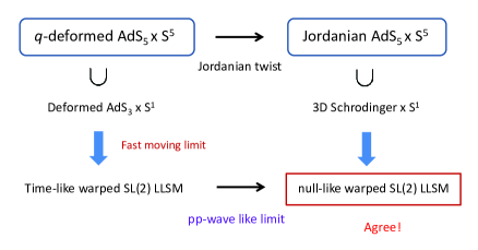
Figure 1: A possible relation between a Jordanian twist and a pp-wave like limit.

The null-like warped $SL(2)$ LLSM is obtained as a pp-wave like limit of the time-like warped one, as explained in Appendix D. The identical null-like warped $SL(2)$ LLSM is also derived from a string sigma model on Sch${}_{3}\times$S¹ . Then the geometry of Sch${}_{3}\times$S¹ is contained as a subspace of a Jordanian deformed AdS${}_{5}\times$S⁵ KMY-JordanianIIB .

Thus one may expect a relation between the $q$-deformed AdS${}_{5}\times$S⁵ and the Jordanian deformed AdS${}_{5}\times$S⁵ . Indeed, this is the case. As explained in detail in KMY-JordanianAdSxS  , the $r$-matrix that leads to the Jordanian deformed solution KMY-JordanianIIB is constructed by performing a Jordanian twist of the $r$-matrix of Drinfeld-Jimbo type DMV-string ; ABF . Hence this observation suggests that the Jordanian twist at the $r$-matrix level corresponds to the pp-wave like limit at the geometry level, as depicted in Figure 1. It would be an interesting issue to make this correspondence more precise.

5 Conclusion and Discussion

In this paper, we have derived anisotropic LLSMs from bosonic subsectors of the $q$-deformed AdS${}_{5}\times$S⁵ superstring action by taking fast-moving string limits. Then we have investigated the classical integrability of the LLSMs from the viewpoint of infinite-dimensional symmetries.

Concretely speaking, we have considered the subsectors, 1) deformed AdS${}_{3}\,\times\,$S¹ and 2) R $\times$ deformed S³ . By taking fast-moving string limits, a time-like warped $SL(2)$ LLSM and a squashed S³ LLSM have been derived for the case 1) and the case 2), respectively. It is remarkable that the resulting LLSMs coincide precisely with the ones obtained from a time-like warped AdS space and a squashed S³ KameYoshi .

Then infinite-dimensional symmetries have been revealed under an appropriate boundary condition. In the case 1), a quantum affine algebra $U_{q}(\widehat{sl(2)})$ has been shown explicitly by computing the Poisson brackets of conserved non-local charges. In the case 2), a quantum affine algebra $U_{q}(\widehat{su(2)})$ is realized. It should be noted that non-ultra local terms do not appear in computing the Poisson algebra and hence there is no ambiguity in studying the classical integrable structure, in comparison to principal chiral models.

For the case 1) , a pp-wave like limit has been applied. The resulting system coincides with a null-like warped $SL(2)$ LLSM obtained as a fast-moving string limit of a string sigma model on Sch${}_{3}\times$S¹ KameYoshi . As a result, a couple of Yangians ${\mathcal{Y}}(sl(2))$ have been revealed by performing non-local gauge transformations which correspond to undoing Jordanian twists. In addition, we have argued a possible relation between the $q$-deformed AdS${}_{5}\times$S⁵ and Jordanian deformed AdS${}_{5}\times$S⁵ .

It is interesting to consider some generalizations of our result. There would be various directions. The first is to consider a long-range generalization . By following the works KRT ; KT ; MTT , it would be possible to argue a long-range generalization of our result (For example, for a long-range generalization of the XXZ model see BFdLL ). The next is to consider larger subsectors, or directly the full sector (For a supersymmetric generalization of the undeformed case, see Rafael2 ; Stefanski ). It would also be nice to consider the LLSMs obtained here at the quantum level, for example, by following RTT ; Tirziu ; quantumLL .

There are many open problems concerning anisotropic LLSMs. We hope that our result would open up a new arena to study $q$-deformations of the AdS${}_{5}\times$S⁵ superstring.

Acknowledgments

We are grateful to Io Kawaguchi for helpful discussions and collaborations at an earlier stage. We also appreciate Niklas Beisert, Marius de Leeuw, Sergey Frolov, Takuya Matsumoto and Matthias Staudacher for useful discussions. The work of TK was supported by the Japan Society for the Promotion of Science (JSPS).

Appendix A Our convention of generators

We shall summarize here our conventions of the $sl(2)$ and $su(2)$ generators.

A.1 The $sl(2)$ generators

The $sl(2)$ generators $T^{a}$’s are defined as

$$T^{0}\equiv\frac{i}{2}\sigma_{2}\,,\quad T^{1}\equiv\frac{1}{2}\sigma_{1}\,,\quad T^{2}\equiv\frac{1}{2}\sigma_{3}\,,$$ (95)

where $\sigma_{i}~{}~{}(i=1,2,3)$ are the standard Pauli matrices. Then the commutation relation and the normalization are

$$\left[T^{a},T^{b}\right]=\varepsilon^{ab}_{~{}~{}c}T^{c}\,,\qquad{\rm Tr}\left(T^{a}T^{b}\right)=\frac{1}{2}\gamma^{ab}\,,$$ (96)

with a totally anti-symmetric tensor $\varepsilon^{ab}_{~{}~{}c}$ normalized as $\varepsilon^{01}_{~{}~{}2}=+1$ . The components of $\gamma^{ab}$ are given by

$$-\gamma^{00}=\gamma^{11}=\gamma^{22}=+1\,,\qquad\gamma^{ab}=0~{}~{}(a\neq b)\,.$$ (97)

The $sl(2)$ indices are raised and lowered by $\gamma^{ab}$ and its inverse, respectively.

It is convenient to introduce $T^{\pm}$ defined as

$$T^{\pm}\equiv\frac{1}{\sqrt{2}}\left(T^{0}\pm T^{1}\right)\,,$$ (98)

where the components of $\varepsilon^{abc}$ and $\gamma^{ab}$ are

$$\varepsilon^{-+2}=+1\,,\qquad-\gamma^{-+}=-\gamma^{+-}=\gamma^{22}=+1\,.$$

It is also helpful to introduce other linear combinations $T^{\widehat{\pm}}$ defined as

$$T^{\widehat{\pm}}\equiv\frac{1}{\sqrt{2}}\left(T^{1}\pm iT^{2}\right)\,,$$ (99)

The commutation relation and the normalization are

$$\left[T^{a},T^{b}\right]=i\,\varepsilon^{ab}_{~{}~{}c}T^{c}\,,\qquad{\rm Tr}\left(T^{a}T^{b}\right)=\frac{1}{2}\gamma^{ab}\,,$$ (100)

where the components of $\varepsilon^{abc}$ and $\gamma^{ab}$ are expressed as

$$\varepsilon^{0{\widehat{-}}{\widehat{+}}}=+1\,,\qquad-\gamma^{00}=\gamma^{\widehat{-}\widehat{+}}=\gamma^{\widehat{+}\widehat{-}}=+1\,.$$

A.2 The $su(2)$ generators

The $su(2)$ generators $T^{a}$’s are defined as

$$T^{1}\equiv\frac{1}{2i}\sigma_{1}\,,\quad T^{2}\equiv\frac{1}{2i}\sigma_{2}\,,\quad T^{3}\equiv\frac{1}{2i}\sigma_{3}\,,$$ (101)

where $\sigma_{i}~{}~{}(i=1,2,3)$ are the standard Pauli matrices. Then the commutation relation and the normalization are given by

$$\left[T^{a},T^{b}\right]=\varepsilon^{ab}_{~{}~{}c}T^{c}\,,\qquad{\rm Tr}\left(T^{a}T^{b}\right)=\frac{1}{2}\delta^{ab}\,,$$ (102)

with a totally anti-symmetric tensor $\varepsilon^{ab}_{~{}~{}c}$ normalized as $\varepsilon^{12}_{~{}~{}3}=+1$ . The $su(2)$ indices are raised and lowered by $\delta^{ab}$ and its inverse, respectively.

It is convenient to introduce $T^{\pm}$ defined as

$$T^{\pm}\equiv\frac{1}{\sqrt{2}}\left(T^{1}\pm iT^{2}\right)\,,$$ (103)

where the components of $\varepsilon^{abc}$ and $\delta^{ab}$ are given by

$$\varepsilon^{-+3}=+1\,,\qquad\delta^{33}=\delta^{{+}{-}}=\delta^{{-}{+}}=+1\,.$$

Appendix B Integrability of squashed S³ LLSM

Here we consider the classical integrability of the squashed S³ LLSM and the associated infinite-dimensional symmetry.

B.1 The classical action and Lax pair

The classical action of the squashed S³ LLSM is given by

$$S = \frac{L}{2}\int^{\infty}_{-\infty}\!\!\!dtdx\,\biggl{[}C\cos^{2}\theta-\cosh\theta\partial_{t}\phi$$ (104)

$$\hskip 85.35826pt-\frac{\lambda}{16\pi^{2}L^{2}}\left[\left(\partial_{x}\theta\right)^{2}+\sin^{2}\theta\left(\partial_{x}\phi\right)^{2}\right]\biggr{]}\,.$$

When $C=0$ , the isotropic $S^{3}$ LLSM is reproduced.

It is convenient to introduce a vector representation with $n^{a}$ . The components are

$$n^{1}=\sin\theta\sin\phi\,,\qquad n^{2}=\sin\theta\cos\phi\,,\qquad n^{3}=\cos\theta\,,$$ (105)

and satisfy a constraint condition,

$$\left(n^{1}\right)^{2}+\left(n^{2}\right)^{2}+\left(n^{3}\right)^{2}=1\,.$$ (106)

Then the classical equations of motion are rewritten as

$$\partial_{t}n^{1}=\frac{\lambda}{8\pi^{2}L^{2}}\left(n^{2}\partial_{x}^{2}n^{3}-n^{3}\partial_{x}^{2}n^{2}\right)+2Cn^{2}n^{3}\,,$$

$$\partial_{t}n^{2}=\frac{\lambda}{8\pi^{2}L^{2}}\left(n^{3}\partial_{x}^{2}n^{1}-n^{1}\partial_{x}^{2}n^{3}\right)-2Cn^{1}n^{3}\,,$$

$$\partial_{t}n^{3}=\frac{\lambda}{8\pi^{2}L^{2}}\left(n^{1}\partial_{x}^{2}n^{2}-n^{2}\partial_{x}^{2}n^{1}\right)\,.$$ (107)

These are equivalent to the Landau-Lifshitz equations

$$\partial_{t}n_{a}=\varepsilon_{abc}n^{b}\left(\dfrac{\lambda}{8\pi^{2}L^{2}}\partial_{x}^{2}n^{c}+\mathcal{J}^{c}_{~{}d}n^{d}\right)\qquad(a=1,2,3)\,,$$ (108)

with an anisotropic matrix $\mathcal{J}$

$$\mathcal{J}^{a}_{~{}b}=\textrm{diag}(j,j,j+2C)\qquad(j:~{}\textrm{an~{}arbitrary~{}const.})\,.$$ (109)

Lax pair and monodromy matrix

Let us introduce the Lax pair of the squashed S³ LLSM FT ,

$$U(t,x;z) = \dfrac{\alpha}{\sin z}\left[n^{1}T^{1}+n^{2}T^{2}+\cos z\,n^{3}T^{3}\right]\,,$$ (110)

$$V(t,x;z) = \dfrac{\beta}{\sin z}\left[\left(n^{2}\partial_{x}n^{3}-n^{3}\partial_{x}n^{2}\right)T^{1}+\left(n^{3}\partial_{x}n^{1}-n^{1}\partial_{x}n^{3}\right)T^{2}\right.$$

$$\hskip 42.67912pt\left.+\cos z\left(n^{1}\partial_{x}n^{2}-n^{2}\partial_{x}n^{1}\right)T^{3}\right]$$

$$-\dfrac{\alpha\beta}{\sin^{2}z}\left[\cos z\,n^{1}T^{1}+\cos z\,n^{2}T^{2}+n^{3}T^{3}\right]\,,$$

where we have introduced a spectral parameter $z\in\mathbb{C}$ and new parameters,

$$\alpha\equiv\dfrac{4\pi L}{\sqrt{\lambda}}\sqrt{C}\,,\qquad\beta\equiv\dfrac{\sqrt{\lambda}}{2\pi L}\sqrt{C}\,.$$ (111)

It is an easy task to check that the equations of motion (107) are reproduced from the commutation relation

$$\Bigl{[}\partial_{t}-V(t,x;z),\partial_{x}-U(t,x;z)\Bigr{]}=0\,.$$ (112)

The monodromy matrix can be introduced as

$$M(z)\equiv{\rm P}\exp\left[\int^{\infty}_{-\infty}\!\!\!dx~{}U(t,x;z)\right]\,,$$ (113)

where $P$ denotes the parth-ordering. This is a conserved quantity again. As we will see later, the expansions around $z=\pm\infty$ lead to a quantum affine algebra $U_{q}(\widehat{su(2)})$ .

B.2 The standard $q$-deformation of $su(2)$

Let us consider a $q$-deformation of $su(2)$ realized in the squashed S³ LLSM.

The $SU(2)$ symmetry of the isotropic S³ LLSM is broken to $U(1)$ due to the deformation. The remaining $U(1)$ generator is given by

$$Q^{3}=-\dfrac{L}{2}\int^{\infty}_{-\infty}\!\!\!dx~{}n^{3}(x)\,.$$ (114)

Note here that the broken components of $SU(2)$ are still realized in a non-local way even when $C\neq 0$ , as in the time-like warped $SL(2)$ LLSM.

To find out the corresponding non-local charges, it is helpful to introduce $n^{{\pm}}$ defined as

$$n^{{\pm}}\equiv\frac{n^{1}\pm in^{2}}{\sqrt{2}}\,.$$ (115)

We take the rapidly damping condition so that $n^{{\pm}}$ vanish at the spatial infinities. The non-local charges are conserved under this boundary condition (See Appendix C).

The non-local conserved charges are given by

$$Q^{{\pm}}=-\dfrac{L}{2}\int^{\infty}_{-\infty}\!\!\!dx~{}{\rm e}^{\alpha\chi(x)}n^{{\pm}}(x)\,,$$ (116)

where $\chi(x)$ is a non-local field defined as

$$\chi(x)\equiv\frac{1}{2}\int^{\infty}_{-\infty}\!\!\!dy\,\epsilon(x-y)\,n^{3}(y)\,.$$ (117)

Here the following relations are useful to show the conservation laws of $Q^{{\pm}}$ ,

$$\partial_{x}\chi=n^{3}\,,\qquad\partial_{t}\chi=i\frac{\lambda}{8\pi^{2}L^{2}}\left(n^{{+}}\partial_{x}n^{{-}}-n^{{-}}\partial_{x}n^{{+}}\right)\,.$$ (118)

The next is to compute the Poisson brackets of $Q^{3}$ and $Q^{{\pm}}$ . The brackets for $n^{a}\,(a=3,{\pm})$ are

$$\Big{\{}n^{a}(x),n^{b}(y)\Bigr{\}}_{\rm P}=-i\frac{2}{L}\,\varepsilon^{ab}_{~{}~{}c}n^{c}(x)\delta(x-y)\,.$$ (119)

Non-ultra local terms are not contained again.

With the brackets (119) , the brackets of $Q^{0}$ and $Q^{{\pm}}$ can be evaluated as

$$\Bigl{\{}Q^{{\pm}},Q^{3}\Bigr{\}}_{\rm P} =\pm iQ^{{\pm}}\,,$$

$$\Bigl{\{}Q^{{+}},Q^{{-}}\Bigr{\}}_{\rm P} =-i\frac{L}{2\alpha}\sinh\Bigl{(}\frac{2\alpha}{L}Q^{3}\Bigr{)}\,.$$

This is a classical analogue of the standard $q$-deformation of $su(2)$ Drinfeld2 ; Jimbo .

In addition, there exists another set of non-local conserved charges,

$$\widetilde{Q}^{{\pm}}=-\dfrac{L}{2}\int^{\infty}_{-\infty}\!\!\!dx~{}{\rm e}^{-\alpha\chi(x)}n^{{\pm}}(x)\,.$$ (121)

These are obtained by changing the sign of $\alpha$ in $Q^{{\pm}}$ . Hence, by construction, $Q^{3}$ and $\widetilde{Q}^{{\pm}}$ also generate another $q$-deformed $su(2)$ algebra,

$$\Bigl{\{}\widetilde{Q}^{{\pm}},{Q}^{3}\Bigr{\}}_{\rm P}=\pm i\widetilde{Q}^{{\pm}}\,,$$ (122)

$$\Bigl{\{}\widetilde{Q}^{{+}},\widetilde{Q}^{{-}}\Bigr{\}}_{\rm P}=-i\dfrac{L}{2\alpha}\sinh\Bigl{(}\dfrac{2\alpha}{L}Q^{3}\Bigr{)}\,.$$

It is possible to show that a quantum affine algebra is generated by $Q^{3}$ , $Q^{{\pm}}$ and $\widetilde{Q}^{{\pm}}$ in the sense of Drinfeld’s first realization Drinfeld1 . The derivation is essentially the same as in the time-like warped LLSM, hence we will not give the derivation.

B.3 The classical $r$-matrix

Finally, let us discuss the classical $r$-matrix from (66). The resulting classical $r$-matrix is of trigonometric type FT ,

$$r(z-w)=\dfrac{2}{L}\dfrac{\alpha}{\sin(z-w)}\Bigl{[}T^{1}\otimes T^{1}+T^{2}\otimes T^{2}+\cos(z-w)T^{3}\otimes T^{3}\Bigr{]}\,,$$ (123)

and satisfies the classical Yang-Baxter equation (68) . This ensures the classical integrability of the squashed S³ LLSM.

Appendix C Boundary conditions and conservation laws

We argue here the relation between boundary conditions and the conservation laws of non-local charges for the time-like warped $SL(2)$ LLSM, the squashed S³ LLSM and the null-like warped $SL(2)$ LLSM.

C.1 Time-like warped $SL(2)$ LLSM

Let us first consider the time-like warped $SL(2)$ LLSM.

We impose the following boundary condition:

$$n^{\widehat{\pm}}(x)\rightarrow 0\qquad\textrm{as}\qquad x\rightarrow\pm\infty\,.$$ (124)

In terms of the coordinates, the boundary condition (124) is expressed as

$$\rho(x)\rightarrow 0\,,\quad\psi(x)\rightarrow\textrm{const.}\quad\textrm{as}\quad x\rightarrow\pm\infty\,.$$ (125)

By using the relation

$$\left(n^{0}\right)^{2}-2n^{\widehat{+}}n^{\widehat{-}}=1\,,$$ (126)

the condition (124) implies that $(n^{0})^{2}\to 1$ as $x\to\pm\infty$ . Because we are working with the parametrization $n^{0}=-\cosh\rho$ , the boundary condition for $n^{0}$ is fixed as follows:

$$n^{0}(x)\rightarrow-1\qquad\textrm{as}\qquad x\rightarrow\pm\infty\,.$$ (127)

It should be noted here that the local charge $Q^{0}$ is not finite and diverges under the condition (127). However, this divergence may have a physical interpretation. The value of $Q^{0}$ is closely related to the length of the spatial direction $x$ of the string world-sheet due to the spin chain interpretation. We are now considering the infinite spatial direction of the string world-sheet, hence the divergence of $Q^{0}$ may be interpreted as a rather natural result.

Let us next check the conservation laws of $Q^{\widehat{\pm}}$ . One can show them as follows:

$$\partial_{t}Q^{\widehat{+}} = -\frac{L}{2}\int^{\infty}_{-\infty}\!\!\!dx~{}\partial_{t}[{\rm e}^{\alpha\chi(x)}n^{\widehat{+}}(x)]$$

$$= -i\frac{\lambda}{16\pi^{2}L}\int^{\infty}_{-\infty}\!\!\!dx~{}\partial_{x}[{\rm e}^{\alpha\chi}(n^{\widehat{+}}\partial_{x}n^{0}-n^{0}\partial_{x}n^{\widehat{+}})]-i\frac{\sqrt{\lambda}}{4\pi}\sqrt{C}\int^{\infty}_{-\infty}\!\!\!dx~{}\partial_{x}[{\rm e}^{\alpha\chi}n^{\widehat{+}}]$$

$$= 0\,,$$

$$\partial_{t}Q^{\widehat{-}} = -\frac{L}{2}\int^{\infty}_{-\infty}\!\!\!dx~{}\partial_{t}[{\rm e}^{\alpha\chi(x)}n^{\widehat{-}}(x)]$$

$$= -i\frac{\lambda}{16\pi^{2}L}\int^{\infty}_{-\infty}\!\!\!dx~{}\partial_{x}[{\rm e}^{\alpha\chi}(n^{0}\partial_{x}n^{\widehat{-}}-n^{\widehat{-}}\partial_{x}n^{0})]+i\frac{\sqrt{\lambda}}{4\pi}\sqrt{C}\int^{\infty}_{-\infty}\!\!\!dx~{}\partial_{x}[{\rm e}^{\alpha\chi}n^{\widehat{-}}]$$

$$= 0\,.$$

Under the condition (124), all of the surface terms have vanished.

Similarly, for another set of non-local charges $\widetilde{Q}^{\widehat{\pm}}$ , the conservation laws are shown as

$$\partial_{t}\widetilde{Q}^{\widehat{+}} = -\frac{L}{2}\int^{\infty}_{-\infty}\!\!\!dx~{}\partial_{t}[{\rm e}^{-\alpha\chi(x)}n^{\widehat{+}}(x)]$$

$$= -i\frac{\lambda}{16\pi^{2}L}\int^{\infty}_{-\infty}\!\!\!dx~{}\partial_{x}[{\rm e}^{-\alpha\chi}(n^{\widehat{+}}\partial_{x}n^{0}-n^{0}\partial_{x}n^{\widehat{+}})]+i\frac{\sqrt{\lambda}}{4\pi}\sqrt{C}\int^{\infty}_{-\infty}\!\!\!dx~{}\partial_{x}[{\rm e}^{-\alpha\chi}n^{\widehat{+}}]$$

$$= 0\,,$$

$$\partial_{t}\widetilde{Q}^{\widehat{-}} = -\frac{L}{2}\int^{\infty}_{-\infty}\!\!\!dx~{}\partial_{t}[{\rm e}^{-\alpha\chi(x)}n^{\widehat{-}}(x)]$$

$$= -i\frac{\lambda}{16\pi^{2}L}\int^{\infty}_{-\infty}\!\!\!dx~{}\partial_{x}[{\rm e}^{-\alpha\chi}(n^{0}\partial_{x}n^{\widehat{-}}-n^{\widehat{-}}\partial_{x}n^{0})]-i\frac{\sqrt{\lambda}}{4\pi}\sqrt{C}\int^{\infty}_{-\infty}\!\!\!dx~{}\partial_{x}[{\rm e}^{-\alpha\chi}n^{\widehat{-}}]$$

$$= 0\,.$$

Thus $\widetilde{Q}^{\widehat{\pm}}$ are also conserved under the condition (124).

Note that all of the non-local charges are finite under the condition (124), while the local charge $Q^{0}$ diverges.

C.2 Squashed S³ LLSM

Next, we consider the squashed S³ LLSM. The argument here is essentially the same as in the case of the time-like warped $SL(2)$ LLSM.

First of all, let us impose the following boundary condition:

$$n^{{\pm}}(x)\rightarrow 0\qquad\textrm{as}\qquad x\rightarrow\pm\infty\,.$$ (128)

In terms of the coordinates, the condition (128) is expressed as

$$\theta(x)\rightarrow 0\,,\quad\phi(x)\rightarrow\textrm{const.}\quad\textrm{as}\quad x\rightarrow\pm\infty\,.$$ (129)

By using the relation

$$\left(n^{3}\right)^{2}+2n^{{+}}n^{{-}}=1\,,$$ (130)

the condition (128) indicates that $(n^{3})^{2}\to 1$ as $x\to\pm\infty$ . Due to the parametrization $n^{3}=\cos\theta$ , the boundary condition for $n^{3}$ is fixed as follows:

$$n^{3}(x)\rightarrow 1\qquad\textrm{as}\qquad x\rightarrow\pm\infty\,.$$ (131)

As a result, the local charge $Q^{3}$ is not finite but diverges again. The divergence may also be interpreted physically, as mentioned before.

The conservation laws of $Q^{{\pm}}$ are shown as

$$\partial_{t}Q^{{+}} = -\frac{L}{2}\int^{\infty}_{-\infty}\!\!\!dx~{}\partial_{t}[{\rm e}^{\alpha\chi(x)}n^{{+}}(x)]$$

$$= -i\frac{\lambda}{16\pi^{2}L}\int^{\infty}_{-\infty}\!\!\!dx~{}\partial_{x}[{\rm e}^{\alpha\chi}(n^{3}\partial_{x}n^{{+}}-n^{{+}}\partial_{x}n^{3})]+i\frac{\sqrt{\lambda}}{4\pi}\sqrt{C}\int^{\infty}_{-\infty}\!\!\!dx~{}\partial_{x}[{\rm e}^{\alpha\chi}n^{{+}}]$$

$$= 0\,,$$

$$\partial_{t}Q^{{-}} = -\frac{L}{2}\int^{\infty}_{-\infty}\!\!\!dx~{}\partial_{t}[{\rm e}^{\alpha\chi(x)}n^{{-}}(x)]$$

$$= -i\frac{\lambda}{16\pi^{2}L}\int^{\infty}_{-\infty}\!\!\!dx~{}\partial_{x}[{\rm e}^{\alpha\chi}(n^{{-}}\partial_{x}n^{3}-n^{3}\partial_{x}n^{{-}})]-i\frac{\sqrt{\lambda}}{4\pi}\sqrt{C}\int^{\infty}_{-\infty}\!\!\!dx~{}\partial_{x}[{\rm e}^{\alpha\chi}n^{-}]$$

$$= 0\,.$$

All of the surface terms have vanished under the condition (128).

Also for $\widetilde{Q}^{\pm}$ , the conservation laws are shown as follows:

$$\partial_{t}\widetilde{Q}^{{+}} = -\frac{L}{2}\int^{\infty}_{-\infty}\!\!\!dx~{}\partial_{t}[{\rm e}^{-\alpha\chi(x)}n^{\widehat{+}}(x)]$$

$$= -i\frac{\lambda}{16\pi^{2}L}\int^{\infty}_{-\infty}\!\!\!dx~{}\partial_{x}[{\rm e}^{\alpha\chi}(n^{3}\partial_{x}n^{{+}}-n^{{+}}\partial_{x}n^{3})]-i\frac{\sqrt{\lambda}}{4\pi}\sqrt{C}\int^{\infty}_{-\infty}\!\!\!dx~{}\partial_{x}[{\rm e}^{-\alpha\chi}n^{{+}}]$$

$$= 0\,,$$

$$\partial_{t}\widetilde{Q}^{{-}} = -\frac{L}{2}\int^{\infty}_{-\infty}\!\!\!dx~{}\partial_{t}[{\rm e}^{-\alpha\chi(x)}n^{\widehat{-}}(x)]$$

$$= -i\frac{\lambda}{16\pi^{2}L}\int^{\infty}_{-\infty}\!\!\!dx~{}\partial_{x}[{\rm e}^{\alpha\chi}(n^{{-}}\partial_{x}n^{3}-n^{3}\partial_{x}n^{{-}})]+i\frac{\sqrt{\lambda}}{4\pi}\sqrt{C}\int^{\infty}_{-\infty}\!\!\!dx~{}\partial_{x}[{\rm e}^{-\alpha\chi}n^{{-}}]$$

$$= 0\,.$$

Thus $\widetilde{Q}^{{\pm}}$ are conserved.

Note that all of the non-local charges are finite, while the local charge diverges.

C.3 Null-like warped $SL(2)$ LLSM

Finally, we consider the null-like warped $SL(2)$ LLSM.

For this case, let us introduce the following boundary condition:

$$n^{-}(x)\,,~{}~{}n^{2}(x)\rightarrow 0\quad\textrm{as}\quad x\rightarrow\pm\infty\,.$$ (132)

In terms of the coordinates, this condition (132) is realized as the condition,

$$\rho(x)\rightarrow\infty\,,\quad\psi(x)\rightarrow\frac{3}{2}\pi\quad\textrm{as}\quad x\rightarrow\pm\infty\,,$$ (133)

where $\rho$ is supposed to diverge logarithmically. From the relation

$$2n^{+}n^{-}-\left(n^{2}\right)^{2}=1\,,$$ (134)

the condition (132) indicates that $n^{+}$ should diverge as $x\to\pm\infty$ .

$$n^{+}(x)\rightarrow-\infty\qquad\textrm{as}\qquad x\rightarrow\pm\infty\,.$$ (135)

Then the non-local charges $Q^{+}$ and $\widetilde{Q}^{+}$ are not finite and diverge. Hence a different component of the non-local charges diverges in comparison to the previous two cases. The difference comes from a pp-wave like limit and the divergence may be basically interpreted as an infinite length of the spatial direction of the string world-sheet.

One can check that $Q^{+}$ and $Q^{2}$ are conserved as follows:

$$\partial_{t}Q^{+} = -\frac{L}{2}\int^{\infty}_{-\infty}\!\!\!dx~{}\partial_{t}[{\rm e}^{\sqrt{C}\alpha\chi(x)}n^{+}(x)]$$

$$= \frac{\lambda}{16\pi^{2}L}\int^{\infty}_{-\infty}\!\!\!dx~{}\partial_{x}[{\rm e}^{\sqrt{C}\alpha\chi}(n^{2}\partial_{x}n^{+}-n^{+}\partial_{x}n^{2})]+\frac{\sqrt{\lambda}}{4\pi}\sqrt{C}\int^{\infty}_{-\infty}\!\!\!dx~{}\partial_{x}[{\rm e}^{\sqrt{C}\alpha\chi}n^{2}]$$

$$= 0\,,$$

$$\partial_{t}Q^{2} = -\frac{L}{2}\int^{\infty}_{-\infty}\!\!\!dx~{}\partial_{t}[{\rm e}^{\sqrt{C}\alpha\chi(x)}n^{2}(x)]$$

$$= \frac{\lambda}{16\pi^{2}L}\int^{\infty}_{-\infty}\!\!\!dx~{}\partial_{x}[{\rm e}^{\sqrt{C}\alpha\chi}(n^{-}\partial_{x}n^{+}-n^{+}\partial_{x}n^{-})]+\frac{\sqrt{\lambda}}{4\pi}\sqrt{C}\int^{\infty}_{-\infty}\!\!\!dx~{}\partial_{x}[{\rm e}^{\sqrt{C}\alpha\chi}n^{-}]$$

$$= 0\,.$$

Under the condition (132), all of the surface terms have vanished. Note that the differential terms are ensured to vanish due to the logarithmic behavior of $\rho$ around the spatial infinities.

The conservation laws of $\widetilde{Q}^{+}$ and $\widetilde{Q}^{2}$ are also shown as follows:

$$\partial_{t}\widetilde{Q}^{+} = -\frac{L}{2}\int^{\infty}_{-\infty}\!\!\!dx~{}\partial_{t}[{\rm e}^{-\sqrt{C}\alpha\chi(x)}n^{+}(x)]$$

$$= \frac{\lambda}{16\pi^{2}L}\int^{\infty}_{-\infty}\!\!\!dx~{}\partial_{x}[{\rm e}^{-\sqrt{C}\alpha\chi}(n^{2}\partial_{x}n^{+}-n^{+}\partial_{x}n^{2})]-\frac{\sqrt{\lambda}}{4\pi}\sqrt{C}\int^{\infty}_{-\infty}\!\!\!dx~{}\partial_{x}[{\rm e}^{-\sqrt{C}\alpha\chi}n^{2}]$$

$$= 0\,,$$

$$\partial_{t}\widetilde{Q}^{2} = -\frac{L}{2}\int^{\infty}_{-\infty}\!\!\!dx~{}\partial_{t}[{\rm e}^{-\sqrt{C}\alpha\chi(x)}n^{2}(x)]$$

$$= \frac{\lambda}{16\pi^{2}L}\int^{\infty}_{-\infty}\!\!\!dx~{}\partial_{x}[{\rm e}^{-\sqrt{C}\alpha\chi}(n^{-}\partial_{x}n^{+}-n^{+}\partial_{x}n^{-})]-\frac{\sqrt{\lambda}}{4\pi}\sqrt{C}\int^{\infty}_{-\infty}\!\!\!dx~{}\partial_{x}[{\rm e}^{-\sqrt{C}\alpha\chi}n^{-}]$$

$$= 0\,.$$

As a result, $\widetilde{Q}^{+}$ and $\widetilde{Q}^{2}$ are conserved under the condition (132).

Note that the non-local charges $Q^{2}$ and $\widetilde{Q}^{2}$ as well as the local charge $Q^{-}$ are finite. However, the non-local charges $Q^{+}$ and $\widetilde{Q}^{+}$ diverge.

Appendix D Null-like warped LLSM from time-like LLSM

We derive here the null-like warped $SL(2)$ LLSM from the time-like warped $SL(2)$ LLSM by taking an appropriate scaling-limit (a pp-wave like limit). The classical equations of motion are first reproduced and then the Lax pair is also derived.

D.1 Equations of motion

The equations of motion of the null-like warped $SL(2)$ LLSM are reproduced from those of the time-like warped $SL(2)$ LLSM by taking a scaling limit.

Recall the equations of motion for the time-like warped $SL(2)$ LLSM,

$$\partial_{t}n^{0}=\frac{\lambda}{8\pi^{2}L^{2}}\left(n^{1}\partial_{x}^{2}n^{2}-n^{2}\partial_{x}^{2}n^{1}\right)\,,$$

$$\partial_{t}n^{1}=\frac{\lambda}{8\pi^{2}L^{2}}\left(n^{0}\partial_{x}^{2}n^{2}-n^{2}\partial_{x}^{2}n^{0}\right)-2\widetilde{C}n^{0}n^{2}\,,$$

$$\partial_{t}n^{2}=\frac{\lambda}{8\pi^{2}L^{2}}\left(n^{1}\partial_{x}^{2}n^{0}-n^{0}\partial_{x}^{2}n^{1}\right)+2\widetilde{C}n^{0}n^{1}\,.$$ (136)

Here we have used $\widetilde{C}$ as a deformation parameter. It is convenient to introduce $n^{\pm}$ as

$$n^{\pm}=\frac{n^{0}\pm n^{1}}{\sqrt{2}}\,.$$ (137)

Then let us rewrite the equations of motion in terms of $n^{\pm}$ with the following rescaling:

$$n^{-}\to\sqrt{\frac{2C}{\widetilde{C}}}\,n^{-}\,,\qquad n^{+}\to\sqrt{\frac{\widetilde{C}}{2C}}\,n^{+}\,.$$ (138)

Finally, by taking the $\widetilde{C}\to 0$ limit with $C$ fixed, the equations of motion are evaluated as

$$\partial_{t}n^{-}=-\frac{\lambda}{8\pi^{2}L^{2}}\left(n^{-}\partial_{x}^{2}n^{2}-n^{2}\partial_{x}^{2}n^{-}\right)\,,$$

$$\partial_{t}n^{2}=-\frac{\lambda}{8\pi^{2}L^{2}}\left(n^{-}\partial_{x}^{2}n^{+}-n^{+}\partial_{x}^{2}n^{-}\right)-2C\left(n^{-}\right)^{2}\,,$$

$$\partial_{t}n^{+}=-\frac{\lambda}{8\pi^{2}L^{2}}\left(n^{2}\partial_{x}^{2}n^{+}-n^{+}\partial_{x}^{2}n^{2}\right)-2Cn^{-}n^{2}\,.$$ (139)

These are equivalent to the equations of motion for the null-like warped LLSM in (71).

D.2 A Lax pair of null-like warped $SL(2)$ LLSM

Let us derive the Lax pair of the null-like warped $SL(2)$ LLSM.

We start from the Lax pair of the time-like warped $SL(2)$ LLSM.

$$U(t,x;z) = \dfrac{i\widetilde{\alpha}}{\sinh z}\left[-\cosh z\,n^{0}T^{0}+n^{1}T^{1}+n^{2}T^{2}\right]\,,$$ (140)

$$V(t,x;z) = \dfrac{i\widetilde{\beta}}{\sinh z}\left[-\cosh z\left(n^{1}\partial_{x}n^{2}-n^{2}\partial_{x}n^{1}\right)T^{0}+\left(n^{0}\partial_{x}n^{2}-n^{2}\partial_{x}n^{0}\right)T^{1}\right.$$

$$\hskip 42.67912pt\left.+\left(n^{1}\partial_{x}n^{0}-n^{0}\partial_{x}n^{1}\right)T^{2}\right]$$

$$+\dfrac{\widetilde{\alpha}\widetilde{\beta}}{\sinh^{2}z}\left[-n^{0}T^{0}+\cosh z\,n^{1}T^{1}+\cosh z\,n^{2}T^{2}\right]\,.$$

Here $\widetilde{\alpha}$ and $\widetilde{\beta}$ are defined as

$$\widetilde{\alpha}\equiv\frac{4\pi L}{\sqrt{\lambda}}\sqrt{\widetilde{C}}\,,\qquad\widetilde{\beta}\equiv\frac{\sqrt{\lambda}}{2\pi L}\sqrt{\widetilde{C}}\,,$$ (141)

and $\widetilde{C}$ is a deformation parameter.

Let us rewrite the Lax pair (140) in terms of $T^{\pm}$ and then rescale $z$ , $n^{\pm}$ and $T^{\pm}$ like

$$z\to i\sqrt{\widetilde{C}}\,z\,,\quad n^{-}\to\sqrt{\frac{2C}{\widetilde{C}}}\,n^{-}\,,\quad n^{+}\to\sqrt{\frac{\widetilde{C}}{2C}}\,n^{+}\,,$$

$$T^{-}\to\sqrt{\frac{2C}{\widetilde{C}}}\,T^{-}\,,\quad T^{+}\to\sqrt{\frac{\widetilde{C}}{2C}}\,T^{+}\,.$$ (142)

Finally, by taking the $\widetilde{C}\to 0$ limit, the following Lax pair is obtained,

$$U(t,x;z) = \dfrac{\alpha}{z}\left(-\left[n^{+}-\frac{Cz^{2}}{2}n^{-}\right]T^{-}+n^{2}T^{2}-n^{-}T^{+}\right)\,,$$

$$V(t,x;z) = \dfrac{\beta}{z}\Biggl{(}-\left[\left(n^{2}\partial_{x}n^{+}-n^{+}\partial_{x}n^{2}\right)-\frac{Cz^{2}}{2}\left(n^{-}\partial_{x}n^{2}-n^{2}\partial_{x}n^{-}\right)\right]T^{-}\Biggr{.}$$ (143)

$$\hskip 28.45274pt+\Biggl{.}\left(n^{-}\partial_{x}n^{+}-n^{+}\partial_{x}n^{-}\right)T^{2}-\left(n^{-}\partial_{x}n^{2}-n^{2}\partial_{x}n^{-}\right)T^{+}\Biggr{)}$$

$$+\dfrac{\alpha\beta}{z^{2}}\left(-\left[n^{+}+\frac{Cz^{2}}{2}n^{-}\right]T^{-}+n^{2}T^{2}-n^{-}T^{+}\right)\,.$$

Here $\alpha$ and $\beta$ have newly been introduced as

$$\alpha=\frac{4\pi L}{\sqrt{\lambda}}\,,\qquad\beta=-\frac{\sqrt{\lambda}}{2\pi L}\,.$$ (144)

From the Lax pair (143), one can reproduce the equations of motion for the null-like warped $SL(2)$ LLSM obtained in KameYoshi .

Appendix E Undoing Jordanian twists

We present here non-local gauge transformations for the Lax pair of the null-like warped $SL(2)$ LLSM. The gauge transformations may be interpreted as undoing Jordanian twists.

Let us start from the following Lax pair,

$$U(t,x;z) = \dfrac{\alpha}{z}\left(-\left[n^{+}-\frac{Cz^{2}}{2}n^{-}\right]T^{-}+n^{2}T^{2}-n^{-}T^{+}\right)\,,$$

$$V(t,x;z) = \dfrac{\beta}{z}\Biggl{(}-\left[\left(n^{2}\partial_{x}n^{+}-n^{+}\partial_{x}n^{2}\right)-\frac{Cz^{2}}{2}\left(n^{-}\partial_{x}n^{2}-n^{2}\partial_{x}n^{-}\right)\right]T^{-}\Biggr{.}$$ (145)

$$\hskip 28.45274pt+\Biggl{.}\left(n^{-}\partial_{x}n^{+}-n^{+}\partial_{x}n^{-}\right)T^{2}-\left(n^{-}\partial_{x}n^{2}-n^{2}\partial_{x}n^{-}\right)T^{+}\Biggr{)}$$

$$+\dfrac{\alpha\beta}{z^{2}}\left(-\left[n^{+}+\frac{Cz^{2}}{2}n^{-}\right]T^{-}+n^{2}T^{2}-n^{-}T^{+}\right)\,.$$

Note that this Lax pair has two poles at $z=0$ and $z=\infty$ .

The isomorphisms of $sl(2)$ algebra,

$$T^{-}\to T^{-}\,,\quad T^{2}\to T^{2}\mp\sqrt{C}zT^{-}\,,\quad T^{+}\to T^{+}\mp\sqrt{C}zT^{2}+\frac{Cz^{2}}{2}T^{-}\,,$$ (146)

transforms the Lax pair (145) into

$$U^{(\pm)}(t,x;z) = \dfrac{\alpha}{z}\left[-\left(n^{+}\pm\sqrt{C}zn^{2}\right)T^{-}+\left(n^{2}\pm\sqrt{C}zn^{-}\right)T^{2}-n^{-}T^{+}\right]\,,$$ (147)

$$V^{(\pm)}(t,x;z) = \dfrac{\beta}{z}\biggl{(}-\left[\left(n^{2}\partial_{x}n^{+}-n^{+}\partial_{x}n^{2}\right)\pm\sqrt{C}z\left(n^{-}\partial_{x}n^{+}-n^{+}\partial_{x}n^{-}\right)\right]T^{-}\Biggr{.}$$

$$\hskip 22.76228pt+\left[\left(n^{-}\partial_{x}n^{+}-n^{+}\partial_{x}n^{-}\right)\pm\sqrt{C}z\left(n^{-}\partial_{x}n^{2}-n^{2}\partial_{x}n^{-}\right)\right]T^{2}$$

$$\hskip 22.76228pt\Biggl{.}-\left(n^{-}\partial_{x}n^{2}-n^{2}\partial_{x}n^{-}\right)T^{+}\biggr{)}$$

$$+\dfrac{\alpha\beta}{z^{2}}\left(-\left[n^{+}\pm\sqrt{C}zn^{2}+Cz^{2}n^{-}\right]T^{-}+\left(n^{2}\pm\sqrt{C}zn^{-}\right)T^{2}-n^{-}T^{+}\right)\,.$$

The resulting Lax pairs $(U^{(\pm)}(z),V^{(\pm)}(z))$ do not diverge at $z=\infty$ any more. Then the asymptotic expressions are given by

$$U^{(\pm)}(t,x;z=\infty) = \pm\sqrt{C}\alpha\left(-n^{2}T^{-}+n^{-}T^{2}\right)\,,$$ (148)

$$V^{(\pm)}(t,x;z=\infty) = \pm\sqrt{C}\beta\left[-\left(n^{-}\partial_{x}n^{+}-n^{+}\partial_{x}n^{-}\right)T^{-}\right.$$

$$\hskip 42.67912pt\left.+\left(n^{-}\partial_{x}n^{2}-n^{2}\partial_{x}n^{-}\right)T^{2}\right]-C\alpha\beta n^{-}T^{-}\,.$$

These are useful to construct non-local gauge transformations.

With the help of (148), non-local functions can be defined as

$${\mathcal{F}}^{(\pm)}(t,x)\equiv{\rm P}\exp\left[\int^{x}_{-\infty}\!\!\!dy~{}U^{(\pm)}(t,y;z=\infty)\right]K^{(\pm)}\,.$$ (149)

These functions are obtained as the solutions of the following differential equations:

$$\partial_{t}{\mathcal{F}}^{(\pm)}=V^{(\pm)}(z=\infty){\mathcal{F}}^{(\pm)}\,,\qquad\partial_{x}{\mathcal{F}}^{(\pm)}=U^{(\pm)}(z=\infty){\mathcal{F}}^{(\pm)}\,.$$ (150)

When solving the differential equations, $K^{(\pm)}$ are introduced as integral constant matrices. It is convenient to take $K^{(\pm)}$ as follows:

$$K^{(\pm)}=\exp\left[\pm\dfrac{2\sqrt{C}\alpha}{L}Q^{-}T^{2}\right]\,.$$ (151)

These choices are basically fixed in Jordanian-KMY by borrowing the knowledge of quantum Jordanian twists. Then the explicit expressions of ${\mathcal{F}}^{(\pm)}$ are given by, respectively,

$${\mathcal{F}}^{(+)}=\exp\left[\sqrt{C}\alpha\chi(x)T^{2}\right]\exp\left[-\sqrt{C}\alpha\left(\xi(x)-\frac{1}{L}Q^{2}\right)T^{-}\right]\exp\left[\frac{\sqrt{C}\alpha}{L}Q^{-}T^{2}\right]\,,$$ (152)

$${\mathcal{F}}^{(-)}=\exp\left[-\sqrt{C}\alpha\chi(x)T^{2}\right]\exp\left[\sqrt{C}\alpha\left(\widetilde{\xi}(x)-\frac{1}{L}\widetilde{Q}^{2}\right)T^{-}\right]\exp\left[-\frac{\sqrt{C}\alpha}{L}Q^{-}T^{2}\right]\,.$$

where $\xi(x)$ and $\widetilde{\xi}(x)$ are non-local fields defined as

$$\xi(x)\equiv\frac{1}{2}\int^{\infty}_{-\infty}\!\!\!dy~{}\epsilon(x-y){\rm e}^{\sqrt{C}\alpha\chi(x)}n^{2}(y)\,,$$ (153)

$$\widetilde{\xi}(x)\equiv\frac{1}{2}\int^{\infty}_{-\infty}\!\!\!dy~{}\epsilon(x-y){\rm e}^{-\sqrt{C}\alpha\chi(x)}n^{2}(y)\,.$$

The next is to see the transformation laws of the Lax pairs $(U^{(\pm)}(z),V^{(\pm)}(z))$ under gauge transformations generated by ${\mathcal{F}}^{(\pm)}$ ,

$${\mathcal{U}}^{(\pm)}(z) = \left({\mathcal{F}}^{(\pm)}\right)^{-1}U(z){\mathcal{F}}^{(\pm)}-\left({\mathcal{F}}^{(\pm)}\right)^{-1}\partial_{x}\,{\mathcal{F}}^{(\pm)}\,,$$ (154)

$${\mathcal{V}}^{(\pm)}(z) = \left({\mathcal{F}}^{(\pm)}\right)^{-1}V(z){\mathcal{F}}^{(\pm)}-\left({\mathcal{F}}^{(\pm)}\right)^{-1}\partial_{t}\,{\mathcal{F}}^{(\pm)}\,.$$

The resulting Lax pairs $({\mathcal{U}}^{(\pm)}(z),{\mathcal{V}}^{(\pm)}(z))$ are explicitly given by

$${\mathcal{U}}^{(+)}(z) = \dfrac{\alpha}{z}\left[-{\mathcal{N}}^{-}T^{+}+{\mathcal{N}}^{2}T^{2}-{\mathcal{N}}^{+}T^{-}\right]\,,$$ (155)

$${\mathcal{V}}^{(+)}(z) = \dfrac{\beta}{z}\Bigl{[}-\left({\mathcal{N}}^{-}\partial_{x}{\mathcal{N}}^{2}-{\mathcal{N}}^{2}\partial_{x}{\mathcal{N}}^{-}\right)T^{+}+\left({\mathcal{N}}^{-}\partial_{x}{\mathcal{N}}^{+}-{\mathcal{N}}^{+}\partial_{x}{\mathcal{N}}^{-}\right)T^{2}$$

$$\hskip 22.76228pt\Bigl{.}-\left({\mathcal{N}}^{2}\partial_{x}{\mathcal{N}}^{+}-{\mathcal{N}}^{+}\partial_{x}{\mathcal{N}}^{2}\right)T^{-}\Bigr{]}+\dfrac{\alpha\beta}{z^{2}}\Bigl{[}-{\mathcal{N}}^{-}T^{+}+{\mathcal{N}}^{2}T^{2}-{\mathcal{N}}^{+}T^{-}\Bigr{]}\,,$$

$${\mathcal{U}}^{(-)}(z) = \dfrac{\alpha}{z}\left[-\widetilde{\mathcal{N}}^{-}T^{+}+\widetilde{\mathcal{N}}^{2}T^{2}-\widetilde{\mathcal{N}}^{+}T^{-}\right]\,,$$

$${\mathcal{V}}^{(-)}(z) = \dfrac{\beta}{z}\Bigl{[}-\left(\widetilde{\mathcal{N}}^{-}\partial_{x}\widetilde{\mathcal{N}}^{2}-\widetilde{\mathcal{N}}^{2}\partial_{x}\widetilde{\mathcal{N}}^{-}\right)T^{+}+\left(\widetilde{\mathcal{N}}^{-}\partial_{x}\widetilde{\mathcal{N}}^{+}-\widetilde{\mathcal{N}}^{+}\partial_{x}\widetilde{\mathcal{N}}^{-}\right)T^{2}$$

$$\hskip 22.76228pt\Bigl{.}-\left(\widetilde{\mathcal{N}}^{2}\partial_{x}\widetilde{\mathcal{N}}^{+}-\widetilde{\mathcal{N}}^{+}\partial_{x}\widetilde{\mathcal{N}}^{2}\right)T^{-}\Bigr{]}+\dfrac{\alpha\beta}{z^{2}}\Bigl{\{}-\widetilde{\mathcal{N}}^{-}T^{+}+\widetilde{\mathcal{N}}^{2}T^{2}-\widetilde{\mathcal{N}}^{+}T^{-}\Bigr{\}}\,,$$

where the components of non-local vectors ${\mathcal{N}}^{a}$ and $\widetilde{\mathcal{N}}^{a}$ are given by

$${\mathcal{N}}^{-}=-\frac{1}{\sqrt{C}\alpha}\textrm{e}^{-\frac{\sqrt{C}\alpha}{L}Q^{-}}\partial_{x}\textrm{e}^{-\sqrt{C}\alpha\chi(x)}\,,\quad{\mathcal{N}}^{2}=\partial_{x}\left[\left(\xi-\frac{1}{L}Q^{2}\right)\textrm{e}^{-\sqrt{C}\alpha\chi(x)}\right]\,,$$ (156)

$${\mathcal{N}}^{+}=\textrm{e}^{\frac{\sqrt{C}\alpha}{L}Q^{-}}\left(\textrm{e}^{\sqrt{C}\alpha\chi(x)}n^{+}(x)-\frac{\sqrt{C}\alpha}{2}\partial_{x}\left[\left(\xi-\frac{1}{L}Q^{2}\right)^{2}\textrm{e}^{-\sqrt{C}\alpha\chi(x)}\right]\right)\,.$$

$$\widetilde{\mathcal{N}}^{-}=\frac{1}{\sqrt{C}\alpha}\textrm{e}^{\frac{\sqrt{C}\alpha}{L}Q^{-}}\partial_{x}\textrm{e}^{\sqrt{C}\alpha\chi(x)}\,,\quad\widetilde{\mathcal{N}}^{2}=\partial_{x}\left[\left(\widetilde{\xi}-\frac{1}{L}\widetilde{Q}^{2}\right)\textrm{e}^{\sqrt{C}\alpha\chi(x)}\right]\,,$$

$$\widetilde{\mathcal{N}}^{+}=\textrm{e}^{-\frac{\sqrt{C}\alpha}{L}Q^{-}}\left(\textrm{e}^{-\sqrt{C}\alpha\chi(x)}n^{+}(x)+\frac{\sqrt{C}\alpha}{2}\partial_{x}\left[\left(\widetilde{\xi}-\frac{1}{L}\widetilde{Q}^{2}\right)^{2}\textrm{e}^{\sqrt{C}\alpha\chi(x)}\right]\right)\,.$$

They satisfy the following relations,

$$2{\mathcal{N}}^{-}{\mathcal{N}}^{+}-\left({\mathcal{N}}^{2}\right)^{2}=1\,,\qquad 2\widetilde{\mathcal{N}}^{-}\widetilde{\mathcal{N}}^{+}-\bigl{(}\widetilde{\mathcal{N}}^{2}\bigr{)}^{2}=1\,.$$ (157)

The monodromy matrices constructed from the Lax pairs $(\mathcal{U}^{(\pm)}(z),\mathcal{V}^{(\pm)}(z))$ lead to a couple of Yangians, as shown in the body of this manuscript. This result indicates that the non-local gauge transformations are nothing but undoing Jordanian twists.

References

• (1) J. M. Maldacena, “The large N limit of superconformal field theories and supergravity,” Adv. Theor. Math. Phys.  2 (1998) 231 [Int. J. Theor. Phys.  38 (1999) 1113]. [arXiv:hep-th/9711200].
• (2) N. Beisert et al., “Review of AdS/CFT Integrability: An Overview,” [arXiv:1012.3982 [hep-th]].
• (3) R. R. Metsaev and A. A. Tseytlin, “Type IIB superstring action in AdS${}_{5}\times$S5 background,” Nucl. Phys. B 533 (1998) 109 [hep-th/9805028].
• (4) I. Bena, J. Polchinski and R. Roiban, “Hidden symmetries of the AdS${}_{5}\times$S5 superstring,” Phys. Rev. D 69 (2004) 046002 [hep-th/0305116].
• (5) M. L$\ddot{\rm u}$scher, “Quantum nonlocal charges and absence of particle production in the two-dimensional nonlinear sigma model,” Nucl. Phys.  B 135 (1978) 1. “Scattering of massless lumps and nonlocal charges in the two-dimensional classical nonlinear sigma model,” Nucl. Phys.  B 137 (1978) 46.
• (6) E. Brezin, C. Itzykson, J. Zinn-Justin and J. B. Zuber, “Remarks about the existence of nonlocal charges in two-dimensional models,” Phys. Lett.  B 82 (1979) 442.
• (7) D. Bernard, “Hidden Yangians in 2-D massive current algebras,” Commun. Math. Phys. 137 (1991) 191.
• (8) N. J. MacKay, “On the classical origins of Yangian symmetry in integrable field theory,” Phys. Lett. B 281 (1992) 90 [Erratum-ibid. B 308 (1993) 444].
• (9) K. Zarembo, “Strings on semisymmetric superspaces,” JHEP 1005 (2010) 002 [arXiv:1003.0465 [hep-th]]; L. Wulff, “Superisometries and integrability of superstrings,” [arXiv:1402.3122 [hep-th]].
• (10) N. Beisert and P. Koroteev, “Quantum deformations of the one-dimensional Hubbard model,” J. Phys. A 41 (2008) 255204 [arXiv:0802.0777 [hep-th]].
• (11) N. Beisert, W. Galleas and T. Matsumoto, “A quantum affine algebra for the deformed Hubbard chain,” J. Phys. A 45 (2012) 365206 [arXiv:1102.5700 [math-ph]].
• (12) B. Hoare, T. J. Hollowood and J. L. Miramontes, “$q$-deformation of the AdS${}_{5}\times$S5 superstring S-matrix and its Relativistic Limit,” JHEP 1203 (2012) 015 [arXiv:1112.4485 [hep-th]]; “Bound states of the $q$-deformed AdS${}_{5}\times$S5 superstring S-matrix,” JHEP 1210 (2012) 076 [arXiv:1206.0010 [hep-th]]; “Restoring unitarity in the $q$-deformed world-sheet S-matrix,” JHEP 1310 (2013) 050 [arXiv:1303.1447 [hep-th]].
• (13) M. de Leeuw, V. Regelskis and A. Torrielli, “The quantum affine origin of the AdS/CFT secret symmetry,” J. Phys. A 45 (2012) 175202 [arXiv:1112.4989 [hep-th]].
• (14) G. Arutyunov, M. de Leeuw and S. J. van Tongeren, “The quantum deformed mirror TBA I,” JHEP 1210 (2012) 090 [arXiv:1208.3478 [hep-th]]; “The quantum deformed mirror TBA II,” JHEP 1302 (2013) 012 [arXiv:1210.8185 [hep-th]].
• (15) I. V. Cherednik, “Relativistically invariant quasiclassical Limits of integrable two-dimensional quantum models,” Theor. Math. Phys.  47 (1981) 422 [Teor. Mat. Fiz.  47 (1981) 225].
• (16) L. D. Faddeev and N. Y. Reshetikhin, “Integrability of the principal chiral field model in (1+1)-dimension,” Annals Phys.  167 (1986) 227.
• (17) J. Balog, P. Forgacs and L. Palla, “A two-dimensional integrable axionic sigma model and T duality,” Phys. Lett. B 484 (2000) 367 [hep-th/0004180].
• (18) S. Schafer-Nameki, M. Yamazaki and K. Yoshida, “Coset construction for duals of non-relativistic CFTs,” JHEP 0905 (2009) 038 [arXiv:0903.4245 [hep-th]].
• (19) I. Kawaguchi and K. Yoshida, “Hidden Yangian symmetry in sigma model on squashed sphere,” JHEP 1011 (2010) 032. [arXiv:1008.0776 [hep-th]].
• (20) I. Kawaguchi, D. Orlando and K. Yoshida, “Yangian symmetry in deformed WZNW models on squashed spheres,” Phys. Lett.  B 701 (2011) 475. [arXiv:1104.0738 [hep-th]]; I. Kawaguchi and K. Yoshida, “A deformation of quantum affine algebra in squashed WZNW models,” to appear in J. Math. Phys. [arXiv:1311.4696 [hep-th]].
• (21) I. Kawaguchi and K. Yoshida, “Hybrid classical integrability in squashed sigma models,” Phys. Lett. B 705 (2011) 251 [arXiv:1107.3662 [hep-th]]; “Hybrid classical integrable structure of squashed sigma models: A short summary,” J. Phys. Conf. Ser.  343 (2012) 012055 [arXiv:1110.6748 [hep-th]].
• (22) I. Kawaguchi, T. Matsumoto and K. Yoshida, “The classical origin of quantum affine algebra in squashed sigma models,” JHEP 1204 (2012) 115 [arXiv:1201.3058 [hep-th]]; “On the classical equivalence of monodromy matrices in squashed sigma model,” JHEP 1206 (2012) 082 [arXiv:1203.3400 [hep-th]].
• (23) I. Kawaguchi and K. Yoshida, “Classical integrability of Schrodinger sigma models and $q$-deformed Poincare symmetry,” JHEP 1111 (2011) 094 [arXiv:1109.0872 [hep-th]].
• (24) I. Kawaguchi and K. Yoshida, “Exotic symmetry and monodromy equivalence in Schrodinger sigma models,” JHEP 1302 (2013) 024 [arXiv:1209.4147 [hep-th]].
• (25) I. Kawaguchi, T. Matsumoto and K. Yoshida, “Schroedinger sigma models and Jordanian twists,” JHEP 1308 (2013) 013 [arXiv:1305.6556 [hep-th]].
• (26) D. Orlando, S. Reffert and L. I. Uruchurtu, “Classical integrability of the squashed three-sphere, warped AdS3 and Schr$\ddot{\rm o}$dinger spacetime via T-Duality,” J. Phys. A 44 (2011) 115401. [arXiv:1011.1771 [hep-th]].
• (27) B. Basso and A. Rej, “On the integrability of two-dimensional models with $U(1)\times SU(N)$ symmetry,” Nucl. Phys. B 866 (2013) 337 [arXiv:1207.0413 [hep-th]].
• (28) D. Orlando and L. I. Uruchurtu, “Integrable superstrings on the squashed three-sphere,” JHEP 1210 (2012) 007 [arXiv:1208.3680 [hep-th]].
• (29) F. Delduc, M. Magro and B. Vicedo, “On classical $q$-deformations of integrable $\sigma$-models,” JHEP 1311 (2013) 192 [arXiv:1308.3581 [hep-th]].
• (30) C. Klimcik, “Yang-Baxter sigma models and dS/AdS T duality,” JHEP 0212 (2002) 051 [hep-th/0210095]; “On integrability of the Yang-Baxter sigma-model,” J. Math. Phys. 50 (2009) 043508 [arXiv:0802.3518 [hep-th]]; “Integrability of the bi-Yang-Baxter sigma model,” [arXiv:1402.2105 [math-ph]]; R. Squellari, “Yang-Baxter $\sigma$ model: Quantum aspects,” Nucl. Phys. B 881 (2014) 502 [arXiv:1401.3197 [hep-th]].
• (31) V. G. Drinfel’d, “Hopf algebras and the quantum Yang-Baxter equation,” Sov. Math. Dokl. 32 (1985) 254.
• (32) M. Jimbo, “A $q$ difference analog of $U(g)$ and the Yang-Baxter equation,” Lett. Math. Phys.  10 (1985) 63.
• (33) V. G. Drinfel’d, “Quantum groups,” J. Sov. Math.  41 (1988) 898 [Zap. Nauchn. Semin.  155, 18 (1986)].
• (34) F. Delduc, M. Magro and B. Vicedo, “An integrable deformation of the AdS${}_{5}\times$S5 superstring action,” Phys. Rev. Lett.  112 (2014) 051601 [arXiv:1309.5850 [hep-th]].
• (35) G. Arutyunov, R. Borsato and S. Frolov, “S-matrix for strings on $\eta$-deformed AdS${}_{5}\times$S5,” JHEP 1404 (2014) 002 [arXiv:1312.3542 [hep-th]].
• (36) B. Hoare, R. Roiban and A. A. Tseytlin, “On deformations of AdS${}_{n}\times$Sn supercosets,” [arXiv:1403.5517 [hep-th]].
• (37) G. Arutynov, M. de Leeuw and S. J. van Tongeren, “On the exact spectrum and mirror duality of the (AdS${}_{5}\times$S5)η superstring,” [arXiv:1403.6104 [hep-th]].
• (38) N. Reshetikhin, “Multiparameter quantum groups and twisted quasitriangular Hopf algebras,” Lett. Math. Phys.  20 (1990) 331.
• (39) A. Stolin and P. P. Kulish, “New rational solutions of Yang-Baxter equation and deformed Yangians,” Czech. J. Phys. 47 (1997) 123 [arXiv:q-alg/9608011]; “Deformed Yangians and Integrable Models,” Czech. J.  Phys. 47 (1997) 1207, [arXiv:q-alg/9708024].
• (40) P. P. Kulish, V. D. Lyakhovsky and A. I. Mudrov, “Extended jordanian twists for Lie algebras,” J. Math. Phys.  40 (1999) 4569 [math/9806014 [math.QA]].
• (41) I. Kawaguchi, T. Matsumoto and K. Yoshida, “Jordanian deformations of the AdS${}_{5}\times$S5 superstring,” JHEP 1404 (2014) 153 [arXiv:1401.4855 [hep-th]].
• (42) I. Kawaguchi, T. Matsumoto and K. Yoshida, “A Jordanian deformation of AdS space in type IIB supergravity,” [arXiv:1402.6147 [hep-th]].
• (43) O. Lunin and J. M. Maldacena, “Deforming field theories with $U(1)\times U(1)$ global symmetry and their gravity duals,” JHEP 0505 (2005) 033 [hep-th/0502086].
• (44) S. Frolov, “Lax pair for strings in Lunin-Maldacena background,” JHEP 0505 (2005) 069 [hep-th/0503201].
• (45) A. Hashimoto and N. Itzhaki, “Noncommutative Yang-Mills and the AdS / CFT correspondence,” Phys. Lett. B 465 (1999) 142 [hep-th/9907166].
• (46) J. M. Maldacena and J. G. Russo, “Large N limit of noncommutative gauge theories,” JHEP 9909 (1999) 025 [hep-th/9908134].
• (47) D. Dhokarh, S. S. Haque and A. Hashimoto, “Melvin Twists of global AdS${}_{5}\times$S5 and their Non-Commutative Field Theory Dual,” JHEP 0808 (2008) 084 [arXiv:0801.3812 [hep-th]].
• (48) T. Matsumoto and K. Yoshida, “Lunin-Maldacena backgrounds from the classical Yang-Baxter equation – Towards the gravity/CYBE correspondence,” [arXiv:1404.1838 [hep-th]].
• (49) T. Matsumoto and K. Yoshida, “Integrability of classical strings dual for noncommutative gauge theories,” [arXiv:1404.3657 [hep-th]].
• (50) M. Kruczenski, “Spin chains and string theory,” Phys. Rev. Lett.  93 (2004) 161602 [hep-th/0311203].
• (51) R. Hernandez and E. Lopez, “The SU(3) spin chain sigma model and string theory,” JHEP 0404, 052 (2004) [hep-th/0403139].
• (52) B. Stefanski, Jr. and A. A. Tseytlin, “Large spin limits of AdS/CFT and generalized Landau-Lifshitz equations,” JHEP 0405 (2004) 042 [hep-th/0404133].
• (53) S. Bellucci, P. -Y. Casteill, J. F. Morales and C. Sochichiu, “SL(2) spin chain and spinning strings on AdS${}_{5}\times$S5,” Nucl. Phys. B 707 (2005) 303 [hep-th/0409086].
• (54) T. Kameyama and K. Yoshida, “String theories on warped AdS backgrounds and integrable deformations of spin chains,” JHEP 1305 (2013) 146 [arXiv:1304.1286 [hep-th]].
• (55) W. -Y. Wen, “Spin chain from marginally deformed AdS${}_{3}\times$S3,” Phys. Rev. D 75 (2007) 067901 [hep-th/0610147].
• (56) G. Arutyunov and S. Frolov, “Foundations of the AdS${}_{5}\times$S5 Superstring. Part I,” J. Phys. A 42 (2009) 254003 [arXiv:0901.4937 [hep-th]].
• (57) L. D. Faddeev and L. A. Takhtajan, “Hamiltonian Methods in the Theory of Solitons” Springer Series in Soviet Mathematics (Springer, New York, 1987).
• (58) J. Lukierski, H. Ruegg, A. Nowicki and V. N. Tolstoi, “Q deformation of Poincare algebra,” Phys. Lett.  B 264 (1991) 331.
• (59) Ch. Ohn, “A $\ast$-product on SL(2) and the corresponding nonstandard quantum-U(sl(2)),” Lett. Math. Phys. 25 (1992) 85.
• (60) M. Kruczenski, A. V. Ryzhov and A. A. Tseytlin, “Large spin limit of AdS${}_{5}\times$S5 string theory and low-energy expansion of ferromagnetic spin chains,” Nucl. Phys. B 692 (2004) 3 [hep-th/0403120].
• (61) M. Kruczenski and A. A. Tseytlin, “Semiclassical relativistic strings in S5 and long coherent operators in N=4 SYM theory,” JHEP 0409 (2004) 038 [hep-th/0406189].
• (62) J. A. Minahan, A. Tirziu and A. A. Tseytlin, “1/J2 corrections to BMN energies from the quantum long range Landau-Lifshitz model,” JHEP 0511 (2005) 031 [hep-th/0510080].
• (63) N. Beisert, L. Fievet, M. de Leeuw and F. Loebbert, “Integrable deformations of the XXZ spin chain,” J. Stat. Mech. 1309 (2013) P09028 [arXiv:1308.1584 [math-ph]].
• (64) R. Hernandez and E. Lopez, “Spin chain sigma models with fermions,” JHEP 0411, 079 (2004) [hep-th/0410022].
• (65) B. Stefanski, Jr., “Landau-Lifshitz sigma-models, fermions and the AdS/CFT correspondence,” JHEP 0707 (2007) 009 [arXiv:0704.1460 [hep-th]].
• (66) R. Roiban, A. Tirziu and A. A. Tseytlin, “Asymptotic Bethe ansatz S-matrix and Landau-Lifshitz type effective 2-d actions,” J. Phys. A 39 (2006) 13129 [hep-th/0604199].
• (67) A. Tirziu, “Quantum Landau-Lifshitz model at four loops: 1/J and 1/J2 corrections to BMN energies,” Phys. Rev. D 73 (2006) 106001 [hep-th/0601139].
• (68) A. Melikyan, A. Pinzul, V. O. Rivelles and G. Weber, “On S-Matrix factorization of the Landau-Lifshitz model,” JHEP 0810 (2008) 002 [arXiv:0808.2489 [hep-th]]; A. Melikyan and A. Pinzul, “On quantum integrability of the Landau-Lifshitz model,” J. Math. Phys.  50 (2009) 103518 [arXiv:0812.0188 [hep-th]].