Robustness of continuous-variable entanglement via geometrical nonlinearity

Abstract

We propose a scheme to generate robust stationary continuous-variable entanglement in optomechanical systems, based on geometrical nonlinearity that occurs for large mechanical displacements. Such nonlinearity is often used to correct the dynamics of the systems in the strong coupling regime. It appears that geometrical nonlinearity enhances the entanglement and shifts its maximum towards high detuning values. Using the experimental parameters, we find that such a scheme generates a very robust entanglement against thermal decoherence even at room temperature. Our results show that geometrical nonlinearity affects entanglement as the optomechanical quantum interface.

I Introduction

After success on the quantum ground state achievable 1 ; 2 , the current challenge now is to know how far quantum theory, bizarre as it is, can allow the observation of quantum effects 3 . A suitable effect that can inform us about this quantum theory’s limit is quantum entanglement, since it is a distinguishing feature that separates quantum from classical physics. Quantum entanglement plays an important role in sharing information in quantum networks 4 ; 5 ; 6 . In Particular, the continuous-variable (CV) entangled quantum states constitute a key element to challenge quantum communication processes such as quantum cryptography 7 , quantum teleportation 8 ; 9 ; 10 , quantum dense coding 11 , and quantum computational tasks 12 .

Many theoretical and experimental schemes have been proposed to generate CV entangled quantum states 13 ; 14 ; 15 ; 16 ; 17 ; 18 . According to the great interest in the nanomechanics during this past decade, optomechanical systems 9 ; 11 ; 19 ; 20 ; 21 ; 22 , superconducting microwave cavities 23 ; 24 , and hybrid systems 25 ; 26 have been very recently used as a tool for generating strong CV entangled quantum states. This consists in coupling the optical and/or microwave mode to the mechanical mode of the resonator that vibrates under the electromagnetic field. There are many configurations that have been proposed to this end. In 19 , stationary entanglement between the optical field and the mechanical mode of a vibrating end mirror is generated from the optical Fabry-Pérot cavity. Strong quantum correlation between the mirror and the optical Stokes sideband is explained in 20 as being generated by a scattering process. The configuration used in 21 consists of a whispering-gallery mode cavity with a movable boundary. Entanglement between the mechanical and radiation modes is achieved in 22 by using a suitable modulation of the driving field. A pulsed field is used to create Einstein-Podolsky-Rosen-type entanglement between the mechanical mode and light pulses and microwave pulses respectively in optomechanical cavity 9 and a microwave cavity, respectively 24 . In 11 , a membrane-in-the-middle geometry is used to generate output entangled light from a fixed end Fabry-Pérot cavity. The optical-microwave quantum interface is used in 25 ; 26 to a produce robust entangled signal that can be used for high-fidelity transfer of quantum states between optical and microwave fields. All these schemes aim to generate robust entangled states against decoherence, which limits their lifetime 5 and their performance in quantum applications. This decoherence is often manifested by various factors such as the stability conditions that place constraints on the magnitude of the effective optomechanical couplings and the thermal noise of the mechanical mode.

Recent experimental studies have shown that a cantilever nanobeam can exhibit both stiffening ($+$) and softening ($-$) geometrical nonlinearity 27 ; 28 . This intrinsic anharmonicity in the mechanical motion of micromechanical and nanomechanical resonators is usually small and therefore only relevant in the regime of large oscillation amplitudes where its contribution becomes important 27 ; 28 . In order to detect quantum behavior, it is a common approach to introduce nonlinearities in the quantum system 29 . It is noteworthy that the dynamics of the purely harmonic quantum system is analogous to its classical dynamics, in the sense that expectation values of canonical observables follow the classical equations of motion. Indeed, stiffening geometrical nonlinearity has being used to squeeze the mechanical mode in optomechanical systems 30 and for both quantum control and quantum information processing 29 whereas softening nonlinearity is shown as a factor that limits some quantum effects in optomechanics 31 ; 32 .

In this paper, motivated by the recent experimental parameters of Ref. 1 , we propose a scheme that generates robust CV entanglement against thermal decoherence. This consists to take into account the geometrical nonlinearity which makes a correction on the dynamics of the resonator, in the limit of large displacements 27 ; 28 ; 29 ; 30 ; 31 . Such a scheme can be extended to superconducting microwave circuits and hybrid systems 26 . Section II describes the system used and details the mathematical tools for the entanglement. We then show, in Sec. III how the geometrical nonlinearity is useful to enhance the entanglement even at room temperature. We summarize in Sec. IV.

II Model and dynamics equations

We study a Fabry-Pérot optomechanical cavity, in which one of the cavity’s mirrors is free to move like a flexural mirror cantilever beam. This system is described, in the rotating-wave approximation picture with respect to $\hbar\omega_{\ell}\alpha^{{\dagger}}\alpha$, by the single-mode Hamiltonian 33 ,

$$\begin{split}H&=\hbar(\Delta_{0}-g_{m}x_{m})\alpha^{{\dagger}}\alpha+\frac{\hbar\Omega_{m}}{4}\left(p_{m}^{2}+x_{m}^{2}-\frac{\beta^{\prime}x_{ZPF}^{2}}{2\Omega_{m}^{2}}x_{m}^{4}\right)\\ &+\hbar E_{0}\left(\alpha+\alpha^{{\dagger}}\right).\end{split}$$ (1)

Here $x_{m}$ and $p_{m}$ are the dimensionless position and momentum operators of the mechanical oscillator related to their counterparts operators of the nanobeam as $x=x_{ZPF}x_{m}$ and $p=\frac{\hbar}{x_{ZPF}}p_{m}$, with $[x_{m},p_{m}]=2i$ and $x_{ZPF}=\sqrt{\frac{\hbar}{2M\Omega_{m}}}$. $\Omega_{m}$ and $M$ are the mechanical frequency and the effective mass of the mechanical mode. The annihilation $\alpha$ and creation $\alpha^{{\dagger}}$ photon operator are defined with respect to $[\alpha,\alpha^{{\dagger}}]=1$. The first term of the Hamiltonian describes both the energy of the cavity mode and the radiation pressure coupling of the rate $g_{m}=\sqrt{2}\omega_{c}\frac{x_{ZPF}}{d_{0}}$, where $\omega_{c}$ and $d_{0}$ are the cavity frequency and cavity length, respectively. The second term is the anharmonic mechanical energy of the nanoresonator with $\frac{\beta^{\prime}x_{ZPF}^{2}x_{m}^{4}}{2\Omega_{m}^{2}}$ the anharmonic term. The third term is the input driving by a laser with frequency $\omega_{\ell}$, where the amplitude of the input laser beam $E_{0}$ is related to the input laser power $P_{0}$ by $|E_{0}|=\sqrt{\frac{2P_{0}\kappa}{\hbar\omega_{\ell}}}$. The laser-cavity detuning is defined as $\Delta_{0}=\omega_{\ell}-\omega_{c}$. The aforementioned nonlinear term occurs in the system when the nanoresonator is subjected to large displacement amplitudes. This comes about because the flexure causes the beam to lengthen, which at large amplitudes adds a significant correction to the overall elastic response of the beam 27 ; 28 ; 29 ; 30 ; 31 . Depending on the sign of this nonlinearity, one distinguishes the softening ($-$) and the stiffening ($+$) nonlinearity which both merge in the nanostructure dynamics. Conceptually, a doubly clamped beam exhibits a stiffening nonlinearity and the cantilever has both stiffening and softening nonlinearity 27 ; 28 . The sign of the nonlinearity depends also on the material nonlinearity. Materials become either stiffer of softer for large strains. At some large deflection, the nanodevices will become affected by the material nonlinearity (further informations are available in 27 ; 28 ). Here, we take into account a softening nonlinearity which merges in the optomechanical coupling between the radiation pressure and the position of the flexural cantilever mirror. The parameters used here, given in Table 1, are those of the system that was recently studied experimentally in Ref. 1 .

$\Omega_{m}/2\pi$	$\Gamma_{m}/2\pi$	$Q_{m}$	$g_{0}/2\pi$	$\kappa/\pi$	$P_{0}$	$T$
$3.6\operatorname{GHz}$	$35\operatorname{kHz}$	$1.05\times 10^{5}$	$910\operatorname{kHz}$	$529\operatorname{MHz}$	$0.7\operatorname{mW}$	$270\operatorname{mK}$

Table 1: Experimental parameters of Ref. 1 used in this work.

Considering the photon losses in the cavity and the Brownian noise acting on the resonator, one derives from the Hamiltonian (1), the nonlinear quantum Langevin equations (QLEs) 31

$$\dot{x}_{m} =\Omega_{m}p_{m},$$ (2a)

$$\dot{p}_{m} =-\Omega_{m}x_{m}-\Gamma_{m}p_{m}+g_{m}\alpha^{{\dagger}}\alpha+\beta^{\prime\prime}+F_{th},$$ (2b)

$$\dot{\alpha} =\left[i(\Delta_{0}+g_{m}x_{m})-\frac{\kappa}{2}\right]\alpha-iE_{0}+\sqrt{\kappa}\alpha^{in},$$ (2c)

where $\beta^{\prime\prime}=\frac{\beta^{\prime}x_{ZPF}^{2}}{\Omega_{m}}x_{m}^{3}$. We have introduced both the vacuum radiation input noise operator $\alpha^{in}$, whose only nonzero correlation function is

$$\langle\alpha^{in}(t)\alpha^{in,{\dagger}}(t^{\prime})\rangle=\delta(t-t^{\prime}),$$ (3)

and the Hermitian Brownian noise operator $F_{th}$, with the correlation function

$$\langle F_{th}(t)F_{th}(t^{\prime})\rangle=\frac{\Gamma_{m}}{\Omega_{m}}\int\frac{d\Omega}{2\pi}e^{-i\Omega(t-t^{\prime})}\Omega\left[\coth\left(\frac{\hbar\Omega}{2k_{B}T}\right)+1\right],$$ (4)

where $k_{B}$ the Boltzmann constant and $T$ the bath temperature.

By setting the time derivatives to zero in the set of nonlinear equations (2), the steady-state values yield $p_{s}=0,x_{s}=2\frac{g_{m}}{\Omega_{m}}n_{s}$ and $|E_{0}|^{2}=n_{s}(\Delta^{2}+\frac{\kappa^{2}}{4})$, where we have set the steady state photon number in the cavity equal to $n_{s}=|\alpha_{s}|^{2}$. Here $\Delta=\Delta_{0}+2\frac{g_{m}^{2}}{\Omega_{m}}n_{s}$ is the effective detuning. One can rewrite each Heisenberg operator as a $c$-number steady-state value plus an additional fluctuation operator with zero-mean value, $p_{m}=p_{s}+\delta p_{m}$, $x_{m}=x_{s}+\delta x_{m}$, and $\alpha=\alpha_{s}+\delta\alpha$. Inserting these expressions into the set of QLEs equations (2), leads to a set of quantum Langevin equations for the fluctuation operators. As the parameter regime relevant for generating optomechanical entanglement is that with a very large input power $P_{0}$, i.e., for strong coupling $|\alpha_{s}|\gg 1$, one can safely neglect the higher order terms of fluctuations 19 .

By introducing the vector of quadrature fluctuations $u(t)=(\delta x_{m}(t),\delta p_{m}(t),\delta I(t),\delta\varphi(t))^{T}$ and the vector of noises $n(t)=(0,F_{th}(t),\sqrt{\kappa}\delta I^{in}(t),\sqrt{\kappa}\delta\varphi^{in}(t))^{T}$ 32 , the linearized QLEs can be written in compact form

$$\dot{u}(t)=Au(t)+n(t),$$ (5)

where

$$A=\begin{pmatrix}0&\Omega_{m}&0&0\\ \Omega_{m}(\beta-1)&-\Gamma_{m}&G&0\\ 0&0&-\frac{\kappa}{2}&-\Delta\\ G&0&\Delta&-\frac{\kappa}{2}\end{pmatrix}.$$ (6)

The term $G=g_{m}|\bar{\alpha}|$ is the effective optomechanical coupling that can generate a significant entanglement in the strong-coupling limit. The parameter $\beta=\frac{3\beta^{\prime}x_{s}^{2}}{\Omega_{m}^{2}}$ is the dimensionless geometrical nonlinearity that is used in the following (refer to 30 ; 31 for more detailed calculations).

By integrating Eq. (5), we obtain

$$u(t)=M(t)u(0)+\int_{0}^{t}dsM(s)n(s),$$ (7)

where $M(t)=\exp(At)$. To analyze the stability of our system, we have used the Routh-Hurwitz criterion which yield the two nontrivial conditions on the system parameters

$$\begin{split}s_{1}&=\Gamma_{m}\kappa\left\{\left[\frac{\kappa^{2}}{4}+(\Omega_{m}-\Delta)^{2}\right]\left[\frac{\kappa^{2}}{4}(\Omega_{m}+\Delta)^{2}\right]\right.\\ &\left.+\Gamma_{m}\left[(\Gamma_{m}+\kappa)\left(\frac{\kappa^{2}}{4}+\Delta^{2}\right)+\kappa\Omega_{m}^{2}\right]\right\}\\ &-\Delta\Omega_{m}G^{2}(\Gamma_{m}+\kappa)^{2}>0,\end{split}$$ (8)

$$s_{2} =\Omega_{m}\left(\Delta^{2}+\frac{\kappa^{2}}{4}\right)+G^{2}\Delta>0.$$ (9)

With respect to physical parameters in Table 1, these stability conditions lead at the blue sideband of the cavity ($\Delta=-\Omega_{m}$) to $G<2.26\times 10^{10}s^{-1}$ or $\alpha_{s}<2.07\times 10^{3}$ while at the red sideband ($\Delta=\Omega_{m}$) one has $G<2.89\times 10^{7}s^{-1}$ or $\alpha_{s}<0.26$. Optomechanical entanglement is then possible within the blue-sideband detuning range where the coupling is strong. Due to Eq. (4), the mirror Brownian noise $F_{th}(t)$ is not $\delta$ correlated and therefore does not describe a Markovian process. However, as the parameters used here lead to a large mechanical factor $Q=\frac{\Omega_{m}}{\Gamma_{m}}\approx 1.05\times 10^{5}\gg 1$, the quantum effects can be achieved. This limit allows $F_{th}(t)$ to be $\delta$ correlated 19 ,

$$\frac{1}{2}\langle F_{th}(t)F_{th}(t^{\prime})+F_{th}(t^{\prime})F_{th}(t)\rangle\approx\Gamma_{m}(2n_{th}+1)\delta(t-t^{\prime}),$$ (10)

where the mean thermal excitation number is set equal to $n_{th}=(e^{\hbar\Omega_{m}/k_{B}T}-1)^{-1}$ and the Markovian process can then be recovered.

Since the quantum noises $F_{th}$ and $\alpha^{in}$ are zero-mean quantum Gaussian noises and the dynamics is linearized, the quantum steady state for the fluctuations is a zero-mean bipartite Gaussian state, fully characterized by its $4\times 4$ correlation matrix which has the components $V_{ij}=\frac{1}{2}\langle u_{i}(\infty)u_{j}(\infty)+u_{j}(\infty)u_{i}(\infty)\rangle$. When the system is stable, using Eq.(7), we obtain

$$V_{ij}=\sum_{kl}\int_{0}^{\infty}ds\int_{0}^{\infty}ds^{\prime}M_{ik}(s)M_{jl}(s^{\prime})\Phi_{kl}(s-s^{\prime}),$$ (11)

where $\Phi_{kl}(s-s^{\prime})=\frac{1}{2}\langle n_{k}(s)n_{\ell}(s^{\prime})+n_{\ell}(s^{\prime})n_{k}(s)\rangle$ is the matrix of stationary noise correlation functions. Using the fact that the three components of $n(t)$ are uncorrelated, we find $\Phi_{kl}(s-s^{\prime})=D_{kl}\delta(s-s^{\prime})$, where $D=\mathrm{diag}[0,\Gamma_{m}(2n_{th}+1),\kappa,\kappa]$ is a diagonal matrix and Eq. (11) becomes $V=\int_{0}^{\infty}dsM(s)DM(s)^{T}$, which leads, for a stable system ($M(\infty)=0$) and after applying Lyapunov’s first theorem 34 , to

$$AV+VA^{T}=-D.$$ (12)

Here $V$ is known as the system covariance matrix (CM) and it contains all information about the steady state. Equation (12) can be straightforwardly solved, but the general exact expression is too cumbersome and will not be reported here.

III Effects of geometrical nonlinearity on stationary entanglement

The entanglement of the steady state can then be quantified by means of the logarithmic negativity $E_{\mathcal{N}}$ 15 which, in the CV case, is defined as 15 ; 16

$$E_{\mathcal{N}}=\max[0,-\ln 2\eta],$$ (13)

where

$$\eta=\sqrt{\frac{\sum(V)-\sqrt{\sum(V)^{2}-4\det V}}{2}},$$ (14)

is the lowest symplectic eigenvalue of the partial transpose of the CM, with $\sum(V)$ expressed in terms of the $2\times 2$ block matrix

$$V=\begin{bmatrix}V_{m}&V_{corr}\\ V_{corr}^{T}&V_{cav}\end{bmatrix},$$ (15)

as $\sum(V)=\det V_{m}+\det V_{cav}-2\det V_{corr}$. The matrix $V_{m}$ is associated with the oscillating mirror, $V_{cav}$ is associated with the cavity mode, and $V_{corr}$ describes the optomechanical correlations. According to Eq.(13), a Gaussian state is entangled ($E_{\mathcal{N}}>0$) if and only if $\eta<\frac{1}{2}$, which is equivalent to Simon’s necessary and sufficient entanglement nonpositive partial transpose criterion for Gaussian states 16 .

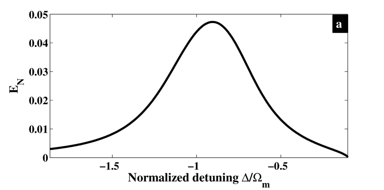
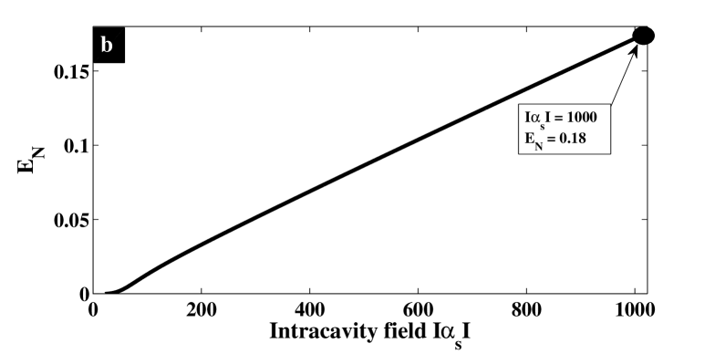
Figure 1: Linear regime obtained with the physical parameters in Table 1. (a) Logarithmic negativity $E_{\mathcal{N}}$ versus normalized detuning $\frac{\Delta}{\Omega_{m}}$. The entanglement is maximal around the blue-detuning $\frac{\Delta}{\Omega_{m}}=-1$. (b) Logarithmic negativity $E_{\mathcal{N}}$ versus intracavity field with high input power $P_{0}=10\operatorname{mW}$. The entanglement is enhanced for high input power.

The parameters of Table 1 not only satisfy our aforementioned stability conditions, but also lead to a generation of a lightly mechanical and optical mode entanglement in linear regime. This entanglement, which is present only in a finite interval of detuning values around the blue-sideband $\frac{\Delta}{\Omega_{m}}=-1$ [Fig.1(a)], can be increased by significant optomechanical coupling as shown in 19 ; 21 ; 23 ; 26 , which consists in increasing,for example, the input power $P_{0}$. This is shown in Fig. 1(b), where the high power is $P_{0}=10\operatorname{mW}$, which corresponds to the intracavity field of $|\alpha_{s}|=10^{3}$, and is in accordance with both current state-of-the-art optics and our stability condition. The above value of the intracavity field has been recently used to generate entangled states 21 and squeezed states 26 in optomechanical systems. Such a high input power induces large mechanical displacement of the nanoresonator, which exhibits a geometrical nonlinearity in the system 29 ; 30 ; 31 .

A more interesting situation is depicted in Fig. 2 (a), which represents the logarithmic negativity versus the normalized detuning for different values of the nonlinear parameter $\beta$. We remarks that the entanglement increment is related to an increase of the nonlinear parameter for $\frac{\Delta}{\Omega_{m}}\in[-1.1;-0.16]$, with a significant enhancement around the normalized detuning $\frac{\Delta}{\Omega_{m}}=-0.5$. In other terms, the entanglement becomes robust with the nonlinearity within the above interval of $\frac{\Delta}{\Omega_{m}}$. In the case where $\beta=0$ (linear case), the optimal entanglement remains near $\Delta=-\Omega_{m}$ (solid black line in Fig. 2(a) and for $\beta\neq 0$ it is shifted towards high detuning values [other curves in Fig.2 (a)]. Reverse effects are induced on entanglement in 19 and 35 by the resonator mass and the Kerr nonlinearity respectively. This means that the softening nonlinear effect study here is a promising way to improve quantum information processing such as quantum teleportation and quantum key distribution. For the small normalized detuning values, $\frac{\Delta}{\Omega_{m}}\in[-2;-1.1]$, the increase of the nonlinearity induces a decrease of the entanglement. However, this opposite effect of the parameter $\beta$ on the entanglement is not important in the system. In Fig. 2 (b) we have set the normalized detuning equal to $\frac{\Delta}{\Omega_{m}}=-0.5$ and varied the nonlinear parameter $\beta$. This curve shows the robustness of entanglement when the nonlinearity increases in the system. Thus, in the system that exhibits geometrical nonlinearity, the optimal entanglement depends on the value of the detuning and should be checked around the detuning $\frac{\Delta}{\Omega_{m}}=-0.5$ but not around $\frac{\Delta}{\Omega_{m}}=-1$ as in linear system 19 .

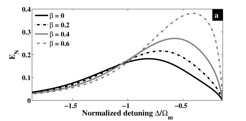
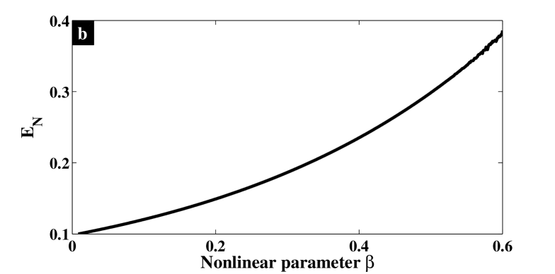
Figure 2: Plots of the input power $P_{0}=10\operatorname{mW}$ and the others parameters are those in Table 1. (a) Logarithmic negativity versus the normalized detuning for different values of geometrical nonlinearity. The increase of nonlinear parameter enhances the entanglement and shifts its maximum value towards high detuning values (compare the gray dash-dotted line and solid black line). (b) Logarithmic negativity versus the geometrical nonlinearity for $\frac{\Delta}{\Omega_{m}}=-0.5$. This shows the robustness of the entanglement in the presence of geometrical nonlinearity.

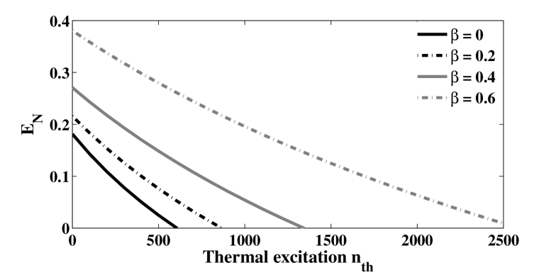
Figure 3: Plot of the logarithmic negativity versus the mean bath occupation for different values of the nonlinear parameter with an input power $P_{0}=10\operatorname{mW}$. This shows the robustness of entanglement against thermal decoherence depending on the nonlinear term. For $\beta=0.6$ this robustness persists to $n_{th}=2500$ (gray dash-dotted line).

Finally, Fig. 3 shows the robustness of the entanglement against the environmental temperature in the presence of such nonlinearity. As expected, in the linear regime ($\beta=0$), there is a decrease of the entanglement with respect to the bath temperature. However, the entanglement persists until $n_{th}=600$ or $T=98\operatorname{K}$, which is several orders of magnitude larger than the temperature needed to cool a mechanical resonator to its quantum ground state. This shows the performance of the system studied here to resist thermal decoherence. Figure 3 mostly reveals that by increasing the geometrical nonlinearity, one definitely improve the robustness of the entanglement against thermal decoherence in an optomechanical system. Indeed, the gray dash-dotted line shows that entanglement persists until $n_{th}=2500$, which corresponds to room temperature. It should be noted that similar results have recently been found in 20 and 26 with the inverse bandwidth and quantum optomechanical interface, respectively. Particularly in 26 , where the hybrid system is studied, the entanglement remains strong even for $n_{th}=10^{4}$, which is greater than that found here ($n_{th}=2500$). This may be understood by the fact that hybrid systems combine two optomechanical couplings, optical and microwave couplings, to drive a nanoresonator.

Since the physical parameters used here have been recently studied experimentally and they satisfy the system’s stability condition for the feasible input power of $P_{0}=10\operatorname{mW}$, our results can then be implemented. This techniques of entanglement that used the geometrical nonlinearity is further promising to observe the quantum effects even for high environmental temperatures. This could lead to the improvement of the robustness of quantum teleportation protocols and other quantum applications.

IV Conclusion

In this work, we have shown that geometrical nonlinearity can be used to enhance the entanglement between the optical intracavity field and the mechanical mode in optomechanical cavities. This nonlinear parameter enables the robustness of the entanglement against thermal decoherence, even at room temperature. With experimental parameters close to those of a recently performed experiment 1 , entanglement persists until $n_{th}=2500$ for an input power of $10\operatorname{mW}$. This scheme offers promising perspectives to produce robust light entangled states for improving quantum information applications such as continuous-variables dense coding, quantum teleportation, quantum cryptography and quantum computational tasks.

References

- (1) J. Chan et al., Nature (London) 478, 89 (2011); M. Sean et al., arXiv:1403.3703.
- (2) A.D. O’Connell et al., Nature (London) 464, 697 (2010).
- (3) K. Hammerer, Science 342, 702 (2013).
- (4) K. Jensen et al., Nat. Phys. 7, 13(2010).
- (5) M. Abdi, S. Pirandola, P. Tombesi and D. Vitali, Phys. Rev. A 89, 022331 (2014).
- (6) R. Horodecki, P. Horodecki, M. Horodecki, and K. Horodecki, Rev. Mod. Phys. 81, 865 (2009).
- (7) D. Stucki et al., New J. Phys. 13, 123001 (2011).
- (8) A. Mari and D. Vitali, Phys. Rev. A 78, 062340 (2008).
- (9) S.G. Hofer, W. Wieczorek, M. Aspelmeyer and K. Hammerer, Phys. Rev. A 84, 052327 (2011).
- (10) C.A. Muschik, K. Hammerer, E.S. Polzik and I.J. Cirac, Phys. Rev. Lett. 111, 020501 (2013).
- (11) S. Barzanjeh, S. Pirandola and C. Weedbrook, Phys. Rev. A 88, 042331 (2013).
- (12) J.Stolze and D. Suter, Quantum Computing: A short course from Theory to Experiment (Wiley-VCH GmbH, Dortmund, 2004).
- (13) M. B. Plenio and S. F. Huelga, Phys. Rev. Lett. 88, 197901-1(2002).
- (14) G. Vidal and R. F. Werner, Phys. Rev. A 65, 032314 (2002).
- (15) G. Adesso, A. Serafini and F. Illuminati, Phys. Rev. A 70, 022318 (2004).
- (16) J. Laurat et al., J. Opt. B: Quantum Semiclass. Opt. 7, 577 (2005).
- (17) D. Vitali, P. Canizares, J. Eschner and G. Morigi, New J. Phys. 10, 033025 (2008).
- (18) I. Sinayskiy, N. Pumulo, and F. Petruccione, arXiv:1401.2306.
- (19) D. Vitali et al., Phys. Rev. Lett. 98, 030405 (2007).
- (20) C. Genes, A. Mari, P. Tombesi and D. Vitali, Phys. Rev. A 78, 032316 (2008).
- (21) Z.-q. Ying and Y-J. Han, Phys. Rev. A 79, 024301 (2009).
- (22) A. Mari and J. Eisert, Phys. Rev. Lett.103, 213603 (2009); New. J. Phys. 14, 075014 (2012).
- (23) D. Vitali, P. Tombesi, M. J. Woolley, A. C. Doherty and G. J. Milburn, Phys. Rev. A 76, 042336 (2007).
- (24) T. A. Palomaki et al., Science 342, 710 (2013).
- (25) Sh. Barzanjeh, M. Abdi, G. J. Milburn, P. Tombesi and D. Vitali, Phys. Rev. Lett.109, 130503 (2012).
- (26) L. Tian, Phys. Rev. Lett.110, 233602 (2013).
- (27) L. G. Villanueva et al., Phys. Rev. B 87, 024304 (2013)
- (28) R.Lifshitz and M.C. Cross, Nonlinear Dynamics of Nanosystems (Wiley-VCH, Weinheim, 2010).
- (29) S. Rips, I. Wilson-Rae and M. J. Hartmann, Phys. Rev. A 89, 013854 (2014); S. Rips and M. J. Hartmann, Phys. Rev. Lett. 110, 120503 (2013).
- (30) X.-Y. Lu, J.-Q. Liao, L. Tian and F. Nori, arXiv: 1403.0049.
- (31) P. Djorwé, J.H. Talla Mbé, S.G. Nana Engo, P. Woafo, Phys. Rev. A 86, 043816 (2012).
- (32) P. Djorwé, S.G. Nana Engo, J.H. Talla Mbé and P. Woafo, Physica B 422, 72 (2013).
- (33) C.K. Law, Phys. Rev. A 51, 2537 (1995).
- (34) P. C. Parks and V. Hahn, Stability Theory (Prentice-Hall, New York, 1993).
- (35) S. Shahidani, M. H. Naderi, M. Soltanolkotabi and S. Barzanjeh, J. Opt. Soc. Am. B 31, 1095 (2014).