Quantum avalanche in the Fe₈ Molecular-Magnet

Abstract

We report spatially resolved, time-dependent, magnetization reversal measurements of an Fe₈ single molecular magnet using a microscopic Hall bar array. We found that under some conditions the molecules reverse their spin direction at a resonance field in the form of an avalanche. The avalanche front velocity is of the order of $1$ m/sec and is sensitive to field gradients and sweep rates. We also measured the propagation velocity of a heat pulse and found that it is much slower than the avalanche velocity. We therefore conclude that in Fe₈, the avalanche front propagates without thermal assistance.

Single molecular magnets (SMM) are an excellent model system for the study of macroscopic quantum phenomena and their interplay with the environment. In recent years, the focus of these studies shifted from single molecule to collective effects. While there are two famous SMM that show quantum behavior, namely, Fe₈ and Mn₁₂, most of the work on collective effects has been focused on Mn₁₂. Indeed, in Mn₁₂ intriguing effects were found, such as deflagration suzuki2005 ; Subedi2013 , quantum assisted deflagration Hernandez2005 , and detonation Detonation . In all these cases, a spin reversal front propagates through the sample as an avalanche. Although showing some signs of quantum behavior Hernandez2005 , these processes are based on over-the-barrier magnetization reversal. Here, we focus on the spin avalanche phenomena in Fe₈, where pure quantum effects exist at dilution refrigerator (DR) temperatures. We measure the avalanche velocity $V_{a}$ for various sweep rates and applied field gradients. We also determine the thermal diffusivity. We find that $V_{a}$ is much faster than the velocity at which heat or matching field propagates through the sample. Moreover, $V_{a}$ is affected by field gradients. Therefore, the avalanche in Fe₈ is a quantum effect sometimes called cold deflagration Garanin2009 . Fe₈ provides the first experimental manifestation of such cold deflagration.

The Fe₈ SMM has spin $S=10$ ground state, as does Mn₁₂. The magnetic anisotropy correspoding to an energy barrier between the spin projection quantum number $m=\pm 10$ and $m=0$ is $27.5$ K WorensdorferScience99 ; Mukhin2001 ; Barra1996 ; Caciuffo1998 ; Park2002 ; in Mn${}_{1}2$ this anisotropy is  $70$ K Caneschi ; Sessoli . Fe₈ molecules show temperature-independent hysteresis loops at $T<400$ mK, with magnetization jumps at matching fields that are multiples of $0.225$ TWernsdorfer2000 ; Wernsdorfer1999 . However, when tunneling is taking place from state $m$ to $m^{\prime}$, where $\left|m^{\prime}\right|\neq 10$, the excited state can decay to the ground state $\left|m^{\prime}\right|=10$, releasing energy in the process. In a macroscopic sample, this energy release can increase the temperature and support a deflagration process by assisting the spin flips. Spontaneous deflagration in Mn₁₂ takes place at various and not necessarily matching fields higher than $1$ T. The deflagration velocity starts from $1$ m/sec and increases with an increasing (static) field up to $15$ m/sec suzuki2005 .

Our avalanche velocity measurements are based on local and time-resolved magnetization detection using a Hall sensor array. The array is placed at the center of a magnet and gradient coils. A schematic view of the array and coils is shown in the inset of Fig. 1. The array is made of Hall bars of dimensions 100$\times$100 $\mu$m² with 100 $\mu$m intervals; the active layer in these sensors is a two-dimensional electron gas formed at the interface of GaAs/AlGaAs heterostructures. The surface of the Hall sensors is parallel to the applied field. Consequently, the effect of the applied field on the sensor is minimal and determined only by the ability to align the array surface and field. The sample and sensors are cooled to $100$ mK using a DR. More details on the Hall measurements can be found in the supplemental material.

A magnetic field gradient could also be produced by two superconducting coils wound in the opposite sense. They are placed at the center of the main coil and produce $0.14$ mT/mm per ampere. Since there is no option of adjusting the sample position after it has been cooled it is reasonable to assume that the sample is not exactly in the center of the main magnet. In addition, the sample has corners and edges. Therefore, a field gradient is expected even when the gradient coils are turned off.

In the experiments, the molecules are polarized by applying a magnetic field of $\pm 1$ T in the $\mathbf{\hat{z}}$ direction. Afterwards, the magnetic field is swept to $\mp 1$ T. The sweep is done at different sweep rates and under various applied magnetic field gradients. During the sweep, the amplified Hall voltage from all sensors and the external field are recorded. From the raw field-dependent voltage of each sensor, a straight line is subtracted. This line is due to the response of the Hall sensor to the external field. The line parameters are determined from very high and very low fields where no features in the raw data are observed.

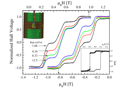
Figure 1: Fe₈ Hysteresis loops for a sample that does not show avalanches at different magnetic field sweep rates. The magnetization is measured via one Hall sensor of the array. The fields for the positive sweep rates are given by the bottom x-axis, and for the negative sweep rates by the top x-axis. The upper inset shows the experimental setup including: 1) sample, 2) Hall sensor array, 3) main coils, 4) gradient coils, and 5) cold finger leading to the Dilution Refrigerator mixing chamber. The lower inset shows the hysteresis loop for a sample that does experience avalanches. Only two magnetization steps are observed in this case.

In our experiments, we found that Fe₈ samples can be divided into two categories: those that do not show avalanches, which have multiple magnetization steps regardless of the sweep rate, and those that show avalanches where the number of magnetization steps depends on the sweep rate. In Fig. 1, we present the normalized Hall voltage as detected by one of the Hall sensors from a sample of the first category. The normalization is by the voltage at a field of 1T where the molecules are fully polarized. Thus, the normalized voltage provides $M/M_{0}$, where M is the magnetization and $M_{0}$ is the saturation magnetization. The bottom abscissa is for a sweep where the field decreases from $1$ T. The top abscissa is for a sweep where the field increases from $-1$ T. The magnetization shows typical steps at intervals of 0.225 T. No step is observed near zero field. In addition, the hysteresis loop’s coercivity increases as the sweep rate increases. These results are in agreement with previous measurements on Fe₈ Wernsdorfer1999 . They are presented here to demonstrate that the Hall sensors are working properly, that their signals indeed represent the Fe₈ magnetization, and that in some samples all magnetization steps are observed.

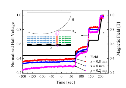
Figure 2: Magnetization as a function of time for a sample of the first type with no avalanche. The magnetization is measured via three different Hall sensors. The field is swept discontinuously. The solid (black) line shows the field value as a function of time on the right y-axis. The magnetization, presented on the left y-axis, changes only when the field changes. The inset demonstrates a tunneling front evolution in a case where the matching field $H_{m}$ moves across the sample during a sweep. $H$ is an instantaneous field intensity. It changes with time and varies in space. The tunneling region with mixed up and down spin has zero magnetization. The expelled magnetic induction $\mathbf{B}$ is detected by the Hall sensors.

The hysteresis loop of a sample from the second category is plotted in the bottom inset of Fig. 1. In this case, there is a small magnetization jump at zero applied field, followed by a nearly full magnetization reversal at a field of $0.2$ T in the form of an avalanche. In all samples tested in this and other experiments in our groupLeviantPhotons , avalanches occurred only at the first matching field. We could not tell in advance whether a sample was of the first or second category. We always worked with samples of approximately the same dimensions ($3\times 3\times 1$ mm³). This is in contrast to Mn₁₂, where avalanches are associated with large samples Garanin .

Avalanche velocity measurements in Fe₈ should be done with extra care. In an avalanche there is, of course, a propagating front where spins flip. But since our measurement in Fe₈ are done by sweeping the field through resonance, there is a similar front even without avalanche. This is demonstrated in the inset of Fig. 2. In this inset, a sample placed off the symmetry point of a symmetric field profile is shown. Thus, the sample experiences a field gradient. Due to this gradient, tunneling of molecules will start first at a particular point in the sample where the local field is at matching value. The spin reversal front will then propagate from that point to the rest of the sample as the external field is swept. In this case, pausing the field sweep will stop the magnetization evolution. This is demonstrated in Fig. 2 for an avalanche free sample. The left ordinate is the normalized Hall voltage (solid symbols) from three different sensors on the array. Each symbol represents a different sensor. The right ordinate is the applied magnetic field (line). The voltage and field are plotted as a function of time. We focus on fields before, near, and after the third transition in Fig. 1. For the most part, the magnetization changes only when the field changes, even in the middle of a magnetization jump. This means that the sample is subjected to some field gradients and a tunneling front propagates through the sample even without an avalanche. It is possible to estimate the matching field front velocity of $V_{m}\sim 1.5\times 10^{-4}$ m/sec from a typical transition width ($0.1$ T), a typical sweep rate ($5$ mT/sec) and the sample length ($3$ mm).

In Fig. 3, we zoom in on the magnetization jump of samples from the second category at a $0.2$ T field. In this figure, we show the time-resolved Hall voltage from five different sensors along the array. The three middle sensors show a peak in the Hall voltage, which is experienced by each sensor at different times. The two outer sensors experience a smoother variation of the Hall voltage, in the form of cusps, also at different times. This type of behavior is a clear indication of a magnetization reversal avalanche propagating from one side of the sample to the other. The peaks and cusps are due to a zero magnetization front, where the magnetization $\mathbf{M}$ changes sign due to tunneling. At the same front, the magnetic induction $\mathbf{B}$ from the sample is forced to point outward and toward the sensors, to maintain zero divergence Friedman2010 . This is demonstrated in the inset of Fig. 2. By following the time evolution of the peaks and cusps, we can determine the front velocity. Since the sensors are spaced by parts of a millimeter and the peaks are spaced by parts of a millisecond, the avalanche velocity $V_{a}$ is of the order of $1$ m/sec, which is much higher than $V_{m}$.

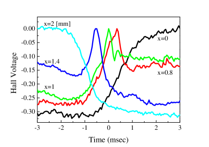
Figure 3: Hall voltage as a function of time for each of the sensors on the array for a sample that has avalanches (as in the inset of Fig. 2). The voltage from each sensor shows a peak or a cusp at different times. The evolution of the peaks and cusps provides the avalanche propagation velocity.

We found that the avalanche propagation direction can be affected by applying field gradients as long as the sweep rate is low. This is demonstrated in Fig. 4. In this figure, we show for each detector location the time at which it experiences a peak or a cusp. The slope of each line is the avalanche velocity. For the lowest sweep rate of 0.83 mT/sec with no gradient, the velocity is negative. It becomes positive as the gradient is switched on to 0.14 mT/mm, but becomes slower as the gradient increases to 0.69 mT/mm. The effect of the gradient is opposite and weaker for our highest sweep rate of 8.3 mT/sec. In this case, all velocities are positive and increase as the gradient increases. Only at the intermediate sweep rate of $1.67$ mT/sec does the gradient have no effect on the velocity. Although we find it challenging to explain the gradient dependence of the avalanche velocity, we do learn from this experiment that the safest sweep rate from which one can estimate the avalanche velocity is around $2$ mT/sec. In this case, the external gradient does not affect the velocity.

The ratio between sweep rates and gradient (when it is on) is a quantity with units of velocity of the order of tens of millimeters per second. This is much lower than $V_{a}$. Therefore, the gradient experiment is another indication, but with an avalanching sample, that the propagation of the external magnetic field does not determine the avalanche velocity, and that $V_{a}$ is an internal quantity of the molecules. In addition, our ability to affect $V_{a}$ with the gradient field rules out the possibility that the avalanche is due to over-the-barrier spin flips.

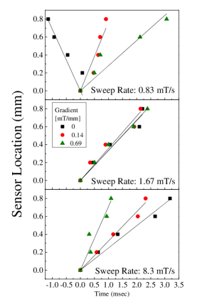
Figure 4: Sensor position as a function of time at which a peak or cusp in the Hall voltage appears for three different sweep rates and three different magnetic field gradients. The slope of each line gives the avalanche velocity.

Finally, in Fig. 5 we depict the avalanche velocities $V_{a}$ as a function of sweep rate with zero applied gradient. The field was swept from positive to negative and vice versa. The sample used in this experiment was of the second category and produced avalanches only for sweep rates higher than 3 mT/sec. Slower sweep rates generated the usual magnetization jumps, as shown in Fig. 1. Although there is some difference between the velocity for different sweep directions, it is clear that the velocity tends to increase with increasing sweep rate, and perhaps saturate. In light of the gradient experiment, the most representative avalanche velocity of Fe₈ is $V_{a}=0.6$ m/sec.

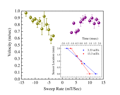
Figure 5: Avalanche velocity as a function of magnetic field sweep rate at zero gradient. The field is swept from positive to negative and vice versa. For sweep rates slower than 3 mT/Sec, no avalanche was observed in this sample. The inset shows raw data of peak position vs. time for two different sweep rates.

To clarify the role of heat propagation in the avalanche process of Fe₈, we also measured the thermal diffusivity $\kappa$ between $300$ mK and $1$ K. This is done by applying a heat pulse on one side of the sample for a duration of $\tau=1$ msec, and measuring the time-dependent temperature on the hot side ($T_{hs}$) and on the cold side ($T_{cs}$) of a sample of length $l\simeq 1$ mm. More experimental details are provided in the supplemental material. The results are shown in Fig. 6. The thermal diffusivity is defined via the heat equation $\frac{\partial T}{\partial t}(x,t)-\kappa\frac{\partial^{2}T(x,t)}{\partial x^{2}}=0$ where $T(x,t)$ is the location and time dependent temperature along the sample. For a long rod $\sqrt{\tau\kappa}\ll l$, one has that

$$\Delta T_{cs}(t)=c\int_{0}^{t}\frac{x\exp\left(-\frac{x^{2}}{4k(t-s)}\right)}{(4\pi\kappa)^{1/2}(t-s)^{3/2}}\Delta T_{hs}(s)ds.$$

We fit this expression to our $T_{cs}(t)$ data with $c$ and $\kappa$ as fit parameters. $c$ accounts for the coupling of the two thermometers to the sample. The fit is shown by the solid line in Fig. 6. Although the fit is not perfect, it does capture the data quite well. The $\kappa$ obtained with this method at a few different temperatures is depicted in the inset of Fig.6. $\kappa$ and $\tau$ obey the long rod condition. It is much smaller than $\kappa$ of Mn₁₂, which is estimated to be $\kappa=10^{-5}$ to $10^{-4}$ m²/sec suzuki2005 . Now, we can generate a heat velocity $V_{h}=\kappa l/A$ where $A$ is the sample cross section. At $T=300$ mK we find that $V_{h}=3\times 10^{-3}$ m/sec. This is roughly $l$ divided by the time between the peak of $T_{hs}(t)$ and that of $T_{cs}(t)$.

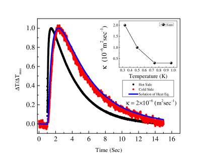
Figure 6: Normalized relative temperature as a function of time at two sides of the sample. Solid line is solution of heat equation for $\kappa=2\times 10^{-6}$. The inset shows thermal diffusivity $\kappa$ at different temperatures

Our experiments show that $V_{a}\gg V_{h}>V_{m}$. This means that the spin reversal front outruns the matching field as it crosses the sample. More important, the avalanche outruns the heat generated in its wake. Every new molecular spin that tunnels does so at the DR temperature. Although heat is produced in the process, this heat does not propel the tunneling front forward. Moreover, the avalanche starts only at the first matching field and it’s velocity is affected by a field gradient. Therefore, the avalanche properties are sensitive to the resonance conditions. All these observations render the avalanche in Fe₈ a quantum mechanical phenomena. The open question is then what sets its velocity. A natural guess, of tunnel splitting $\Delta=4\times 10^{3}$ sec^-1 times unite cell size of $1.6$ nm, namely, $6\times 10^{-6}$ m/sec is too slow WorensdorferScience99 . Therefore, to address this question, more profound considerations have to be taken into account.

This study was partially supported by the Russell Berrie Nanotechnology Institute, Technion, Israel Institute of Technology.

I Supplemental material

The Hall sensor array resides in the center of a printed circuit board (PCB). There is a hole in the PCB and the Hall sensor is glued directly on a copper plate cold finger, which extends from the DR mixing chamber. Gold wire bonding connects the sensors and the leads on the PCB. All wires are thermally connected to the MC. Typical sample dimensions are 3 $\times$ 2 $\times$ 1 mm³. The samples have clear facets and are oriented with the easy axis parallel to the applied field. They are covered by a thin layer of super glue and placed directly on the surface of the Hall sensor with Apizon-N grease, which is used to protect the sample from disintegration and hold it in place. The array backbone has a resistance of $3-4$ k$\Omega$ at our working temperatures, and is excited with a 10$~{}\mu$A DC current. No effect of the sensors’ excitation on the DR-mixing chamber temperature was detected. The Hall voltage from each sensor is filtered with a 30 Hz low-pass filter for hysteresis measurements and a 200 Hz high-pass filter for the avalanche measurements. The voltage is amplified $500$ times by a differential amplifier. It is digitized with an NI USB 6251 A/D card at a rate of $50$ Hz and $20$ KHz for the hysteresis and avalanche measurements respectively.

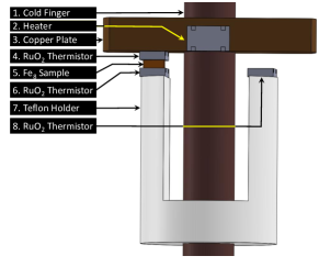
Figure 7: Thermal diffusivity experimental setup. Heat pulse is provided by heater $2$. Thermistor $4$ measures $T_{hs}$ and Thermistor $6$ measures $T_{cs}$. Thermistor $8$ is used to determine heat leaks via the measurement wires.

The thermal diffusivity measurements are performed using two thermometers mounted on opposite sides of the sample and a heater on the hot side of the sample,whose configuration is shown in Fig.7. The hot side is attached to the cold finger and is hot only after the heat pulse. The thermometers are RuO₂ films. The heater is a 2.2K$\Omega$ resistor. The hot side thermometer is between the heater and the sample. The cold side thermometer is between the sample and a teflon plate. It has a weak thermal link to the cold plate via the measurement wires only. A heat pulse is generated by applying $8$ V to the 2.2K$\Omega$ resistor using a function generator, which also gives the trigger for the RuO₂ voltage measurement. The system has been tested by repeating the measurement without the sample to ensure that the recorded heat on the cold side flows through the sample and not through the wires.

References

- (1) Caneschi A, Gatteschi D, Sessoli R, Barra AL, Brunel LC, Guillot M. 1991. J. Am. Chem. Soc. 113:5873
- (2) Sessoli R, Tsai H-L, Schake AR,Wang S, Vincent JB, et al. 1993. J. Am. Chem. Soc. 115:1804
- (3) Y. Suzuki, M. P. Sarachik, E. M. Chudnovsky, S. McHugh, R. Gonzalez-Rubio,N. Avraham, Y. Myasoedov, E. Zeldov, H. Shtrikman, N. E. Chakov and G. Christou, Phys. Rev. Lett. 95, 147201 (2005).
- (4) P. Subedi, S. Vélez, F. Maciá, S. Li, M. P. Sarachik, J. Tejada, S. Mukherjee, G. Christou, and A. D. Kent, Phys. Rev. Lett. 110, 207203 (2013).
- (5) A. Hernández-Mínguez,1 J. M. Hernandez,1 F. Macià,1 A. García-Santiago, J. Tejada, and P.V. Santos, Phys. Rev. Lett 95, 217205 (2005).
- (6) D. A. Garanin and E. M. Chudnovsky,Phys. Rev. Lett. 102, 097206 (2009). ; D. A. Garanin, Phys. Rev. B80, 014406 (2009).
- (7) W. Decelle, J. Vanacken, and V.V. Moshchalkov, J. Tejada, J. M. Hernández, and F. Macià, Phys. Rev. Lett. 102, 027203 (2009); M. Modestov, V. Bychkov, and M. Marklund Phys. Rev. Lett. 107, 207208 (2011).
- (8) W. Wernsdorfer, R. Sessoli, A. Caneschi, D. Gatteschi, A. Cornia, and D. Mailly, J. Appl. Phys. 87, 5481 (2000).
- (9) A Caneschi, D Gatteschi, C Sangregorio, R Sessoli, L Sorace, A Cornia, M.A Novak, C Paulsen, W Wernsdorfer, Journal of Magnetism and Magnetic Materials, Volume 200, Issues 1–3, October 1999, Pages 182-201.
- (10) T. Leviant, in preparation.
- (11) D. A. Garanin and E. M. Chudnovsky,Phys. Rev. B76, 054410 (2007).
- (12) W. Wernsdorfer and R. Sessoli, Science 284, 133 (1999);
- (13) A. Mukhin, B. Gorshunov, M. Dressel, C. Sangregorio, and D. Gatteschi, Phys. Rev. B 63, 214411 (2001)
- (14) A.-L. Barra, P. Debrunner, D. Gatteschi, Ch. E. Schulz, and R. Sessoli, Europhys. Lett. 35, 133 (1996).
- (15) R. Caciuffo, G. Amoretti, A. Murani, R. Sessoli, A. Caneschi, and D. Gatteschi, Phys. Rev. Lett. 81, 4744 (1998).
- (16) K. Park, M. A. Novotny, N. S. Dalal, S. Hill, and P. A. Rikvold, Phys. Rev. B 66, 144409 (2002).
- (17) A. D. Kent et al., Europhys. Lett. 49, 521 (2000).
- (18) E. del Barco, A.D. Kent, S. Hill, J.M. North, N.S. Dalal, E. Rumberger, D.N. Hendrikson, N. Chakov, and G. Christou, J. Low Temp. Phys. 140, 119 (2005).
- (19) J. R. Friedman and M. P. Sarachik, Annu. Rev. Condens. Matter Phys. 1, 109 (2010)