Dynamics of Monopole Walls

Abstract

The moduli space of centred Bogomolny-Prasad-Sommmerfield 2-monopole fields is a 4-dimensional manifold ${\cal M}$ with a natural metric, and the geodesics on ${\cal M}$ correspond to slow-motion monopole dynamics. The best-known case is that of monopoles on ${\mathbb{R}}^{3}$, where ${\cal M}$ is the Atiyah-Hitchin space. More recently, the case of monopoles periodic in one direction (monopole chains) was studied a few years ago. Our aim in this note is to investigate ${\cal M}$ for doubly-periodic fields, which may be visualized as monopole walls. We identify some of the geodesics on ${\cal M}$ as fixed-point sets of discrete symmetries, and interpret these in terms of monopole scattering and bound orbits, concentrating on novel features that arise as a consequence of the periodicity.

1 Introduction

The observation that the dynamics of Bogomolny-Prasad-Sommmerfield (BPS ) monopoles can be approximated as geodesics on the moduli space ${\cal M}$ of static solutions [1] has proved to be far-reaching. Not only does it reveal much about monopole dynamics, but the moduli spaces themselves are of considerable interest, for example in string theory. The best-known case is that of the centred 2-monopole system on ${\mathbb{R}}^{3}$, where ${\cal M}$ is a 4-dimensional asymptotically-locally-flat (ALF) space, namely the Atiyah-Hitchin manifold [2, 3]. For monopoles periodic in one direction, in other words on ${\mathbb{R}}^{2}\times S^{1}$, the asymptotic behaviour of the centred 2-monopole moduli space is different, and is called ALG [4]. In this case, the generalized Nahm transform has been used to describe some of the geodesics on the moduli space, and their interpretation in terms of periodic monopole dynamics [5, 6].

This paper focuses on the doubly-periodic case, namely BPS monopoles on $T^{2}\times{\mathbb{R}}$, also referred to as monopole walls [7, 8]. An $N$-monopole field which is periodic in the $x$- and $y$-directions may be viewed as a set of $N$ monopole walls, each extended in the $xy$-direction. Much is known about the general classification of the moduli spaces of such solutions, and their string-theoretic interpretation [8, 9]. We shall restrict our attention here to the case of smooth 2-monopole fields with gauge group SU(2); the centred moduli space ${\cal M}$ is then a four-dimensional hyperkähler manifold with so-called ALH boundary behaviour [10]. The asymptotic form of its metric has recently been derived [11]. Our aim here is to identify some of the geodesics on ${\cal M}$ as fixed-point sets of discrete symmetries, and to interpret these in terms of monopole scattering, concentrating on novel features that arise as a consequence of the periodicity.

The system, therefore, consists of a smooth SU(2) gauge potential $A_{j}$ on $T^{2}\times{\mathbb{R}}$, plus a Higgs field $\Phi$ in the adjoint representation. The fields satisfy the Bogomolny equation $D_{j}\Phi=-B_{j}$, where $B_{j}={\scriptstyle\frac{1}{2}}\varepsilon_{jkl}F_{kl}$ is the SU(2) magnetic field. The coordinates are $x^{j}=(x,y,z)$, where $x$ and $y$ are periodic with period $1$, and $z\in{\mathbb{R}}$. The boundary condition (see [7, 8] for more detail) is $|\Phi|/|z|\to{\rm const}$ as $z\to\pm\infty$. There are two topological charges $Q_{\pm}$, which are non-negative integers defined in terms of the winding number of $\Phi$. More precisely, if $\Phi_{c}:=\Phi|_{z=c}$, then $\hat{\Phi}_{c}:=\Phi_{c}/|\Phi_{c}|$ is a map from $T^{2}$ to $S^{2}$, and we define $Q_{\pm}:=\pm\deg\hat{\Phi}_{\pm c}$ for $c\gg 1$. The number of monopoles is $N=Q_{+}+Q_{-}$, and we are interested in the case $N=2$, so there are three possibilities, namely $(Q_{-},Q_{+})=(1,1)$, $(0,2)$ or $(2,0)$. In fact, the corresponding moduli spaces are isometric [9]. In what follows, we shall concentrate on the $(1,1)$ wall, namely $Q_{-}=Q_{+}=1$.

2 Parameters and moduli of the $(1,1)$ wall

We begin by reviewing the parameters, the moduli, the energy, and the spectral data of the $(1,1)$ wall, using the same conventions and notation as in [8]. There exists a (non-periodic) gauge such that the boundary behaviour of the fields is

$$\Phi\sim 2\pi{\mathrm{i}}(z+M_{\pm})\sigma_{3},\quad A_{j}\to\pi{\mathrm{i}}(y-2p_{\pm},-x-2q_{\pm},0)\sigma_{3}$$ (1)

as $z\to\pm\infty$. The six real constants $(M_{\pm},p_{\pm},q_{\pm})$ are the boundary-value parameters, with $M_{\pm}\in{\mathbb{R}}$ and $p_{\pm},q_{\pm}\in(-{\scriptstyle\frac{1}{2}},{\scriptstyle\frac{1}{2}}]$. Fixing the centre-of-mass of the system amounts to fixing $(M_{-},p_{-},q_{-})$ in terms of the other three parameters $(M_{+},p_{+},q_{+})$. Henceforth, we fix the centre-of-mass to be at the point $(x,y,z)=({\scriptstyle\frac{1}{2}},{\scriptstyle\frac{1}{2}},0)$, and the field is then invariant (up to a gauge transformation) under the map $(x,y,z)\mapsto(1-x,1-y,-z)$ plus $\Phi\mapsto-\Phi$. In effect, the system as a whole has infinite mass, and only the relative separation and phase of the two monopoles appear in the moduli space; the space of fields with fixed $(M_{\pm},p_{\pm},q_{\pm})$, modulo gauge transformations, is our four-dimensional moduli space ${\cal M}$.

The energy density is ${\cal E}=|D\Phi|^{2}+|B|^{2}$, and ${\cal E}\to 8\pi^{2}$ as $z\to\pm\infty$. The total energy, ie. ${\cal E}$ integrated over $T^{2}\times{\mathbb{R}}$, is consequently infinite. But the cut-off energy

$$E_{L}=\int_{-L}^{L}dz\,\int\left(|D\Phi|^{2}+|B|^{2}\right)\,dx\,dy$$ (2)

is finite, and if $L\gg-M_{+}$ it equals the Bogomolny bound [7]

$$E_{L}=16\pi^{2}(L+M_{+}).$$ (3)

Spectral data for this system may be defined as follows [8]. Put

$$W_{x}=\mathop{\mathrm{tr}}\nolimits{\cal P}\exp\int_{0}^{1}(-A_{x}-{\mathrm{i}}\Phi)\,dx,\quad W_{y}=\mathop{\mathrm{tr}}\nolimits{\cal P}\exp\int_{0}^{1}(-A_{y}-{\mathrm{i}}\Phi)\,dy.$$

Then $W_{x}$ and $W_{y}$ have the form

$$W_{x}=W_{x}(s) = (s+s^{-1})\exp[2\pi(M_{+}+{\mathrm{i}}p_{+})]+2D_{x},$$ (4)

$$W_{y}=W_{y}(\tilde{s}) = (\tilde{s}+\tilde{s}^{-1})\exp[2\pi(M_{+}+{\mathrm{i}}q_{+})]+2D_{y},$$ (5)

where $s=\exp[2\pi(z-{\mathrm{i}}y)]$ and $\tilde{s}=\exp[2\pi(z+{\mathrm{i}}x)]$, and where $D_{x}$, $D_{y}$ are complex constants. The real and imaginary parts of $D_{x}$ and $D_{y}$ are moduli; but they are not independent, so do not provide all the moduli.

The Nahm transform maps walls to walls, although in general the gauge group, the topological charges, and the number of Dirac singularities change [8, 9]. In our case, however, these properties do not change: the Nahm transform of a smooth SU(2) wall of charge $(1,1)$ is again of that type. The action of a Nahm transform on the parameters and the moduli is as follows:

$$(M_{+},p_{+},q_{+}) \mapsto (-M_{+},-p_{+},-q_{+}),$$ (6)

$$D_{x} \mapsto -D_{x}\exp[-2\pi(M_{+}+{\mathrm{i}}p_{+})],$$ (7)

$$D_{y} \mapsto -D_{y}\exp[-2\pi(M_{+}+{\mathrm{i}}q_{+})]).$$ (8)

These expressions follow from the fact that the $x$-spectral curve, given by $t^{2}-tW_{x}(s)+1=0$, is invariant under the Nahm transform, which acts by interchanging the variables $t$ and $s$; and similarly for the $y$-spectral curve [8].

3 The asymptotic region of ${\cal M}$

In order to understand the role played by the parameters and the moduli, let us first look at the asymptotic region of moduli space ${\cal M}$, which consists of those fields for which $|\Phi|_{z=0}\gg 1$. It follows from this condition that $D_{x}$ and $D_{y}$ have the approximate form

$$D_{x}\approx\cosh[2\pi(M+{\mathrm{i}}p)],\quad D_{y}\approx\cosh[2\pi(M+{\mathrm{i}}q)],$$ (9)

with $M\gg\max\{1,M_{+}\}$. Three of the four asymptotic moduli are $M$ and $p,q\in(-{\scriptstyle\frac{1}{2}},{\scriptstyle\frac{1}{2}}]$. The walls are located at values of $z$ for which $W_{x}(s)$ has zeros, and we see from (4) that this occurs for $z=z_{\pm}=\pm(M-M_{+})$; so we have two well-separated walls. Note that $|D_{x}|\approx|D_{y}|$ up to exponentially small corrections, so we could equally well have used the zeros of $W_{y}(\tilde{s})$ to define the wall locations; but this is only true asymptotically, and not in the core region of ${\cal M}$. Each wall has a monopole embedded in it, the monopole locations ${\bf R}_{\pm}=(x_{\pm},y_{\pm},z_{\pm})$ being defined to be where $W_{x}(s)=0=W_{y}(\tilde{s})$. Numerical solutions indicate that this is where $\Phi$ is zero, and also where the energy density is peaked. It follows from (4, 5) that the location of the $z>0$ monopole is ${\bf R}_{+}=({\scriptstyle\frac{1}{2}}+q-q_{+},{\scriptstyle\frac{1}{2}}-p+p_{+},M-M_{+})$.

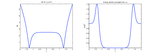
Figure 1: Higgs field and energy density of a well-separated two-wall solution

The energy density is approximately zero for $z_{-}<z<z_{+}$ (between the two walls), and tends to $8\pi^{2}$ as $z\to\pm\infty$. See Fig 1, which depicts a solution with $M_{+}=-0.92$ and $D_{x}=D_{y}=6.21$; this solution was obtained numerically by minimizing the functional (2). The left-hand plot is of $|\Phi|$ on the line $x=y={\scriptstyle\frac{1}{2}}$, where the monopoles are located. The right-hand plot is of the normalized, $xy$-averaged energy density $(8\pi^{2})^{-1}\int{\cal E}\,dx\,dy$, as a function of $z$. Between the walls, the function $|\Phi|$ is approximately constant; in fact $|\Phi|\approx 2\pi M$.

In view of the shape of the energy density, one might have expected that $E_{L}$ could be reduced by moving the walls further apart, ie. by increasing $M$: it looks like an increase $\delta M$ in $M$ would give $\delta E_{L}=-16\pi^{2}\,\delta M$, as the central region (where ${\cal E}$ is zero) increases in size. But in fact as $M$ increases and the walls move apart, the energy contained in each monopole increases by $8\pi^{2}\,\delta M$. This is because each monopole resembles an ${\mathbb{R}}^{3}$ monopole with $|\Phi|_{\infty}=2\pi M$ and therefore energy $8\pi^{2}M$. So the total energy $E_{L}$ is independent of $M$, as it must be from (3). Note, however, that stability involves fixing the value of the parameter $M_{+}$, and reducing $M_{+}$ really does lower the energy. This is analogous to having to fix the boundary value of $|\Phi|$ in the ${\mathbb{R}}^{3}$ case.

Furthermore, the size of each monopole core is proportional to $M^{-1}$, and therefore one may think of them as small SU(2) monopoles embedded in an ambient U(1) field. So the asymptotic moduli are analogous to those of the ${\mathbb{R}}^{3}$ case: three moduli $(M,p,q)$ determine the relative location of the two monopoles, and the fourth is a relative phase $\omega\in(-\pi,\pi]$ between them. The asymptotic metric, in our coordinates $(M,p,q,\omega)$, takes the hyperkähler form [11]

$$ds^{2}=\pi W(dM^{2}+dp^{2}+dq^{2})+\pi W^{-1}[d\omega-8\pi(q\,dp-p\,dq)]^{2},$$ (10)

where $W=W(M)=8\pi(2M-M_{+})$. Here, for simplicity, we have set $p_{+}=q_{+}=0$. Note from (10) that $R=M^{3/2}$ is an affine parameter on asymptotic ‘radial’ geodesics $p,q,\omega$ constant. The volume ${\rm Vol}_{R}$ of a ball of radius $R$ scales like ${\rm Vol}_{R}\sim R^{4/3}$, and so ${\cal M}$ is of ALH type [10].

4 The interior of ${\cal M}$

If $M_{+}\gg 1$, then the monopoles are always well-localized: the monopole size is small compared to unity even when the walls are close together. The energy density is strongly peaked at the locations of the two monopoles, one in each wall; if the monopoles coincide, the energy is peaked on a well-localized torus. So we expect that for $M_{+}\gg 1$, we can interpret the moduli space in terms of the locations and relative phase of the two monopoles, taking account of the periodicity in the $x$- and $y$-directions. If $M_{+}\ll-1$, the moduli space should be the same (via the Nahm transform), although the corresponding monopole picture will differ; in particular, the monopoles in this case will not be well-localized when the walls are close together.

For the case when $M_{+}$ is close to zero, one may also get information by looking at a neighbourhood of the one explicit solution which is known, namely the constant-energy solution. In a non-periodic gauge, this is

$$\Phi_{(0)}=2\pi{\mathrm{i}}z\,\sigma_{3},\quad A_{(0)j}=\pi{\mathrm{i}}(y,-x,0)\,\sigma_{3}.$$ (11)

It has parameters $M_{+}=p_{+}=q_{+}=0$ and moduli $D_{x}=D_{y}=0$, and its energy density has the constant value $8\pi^{2}$. To understand nearby solutions, we examine perturbations of (11); details have appeared in [8], and we summarize them here in a slightly different form.

If $\varepsilon$ is an infinitesimal parameter, take the Higgs field to be $\Phi=\Phi_{(0)}+\varepsilon\Phi_{(1)}+\varepsilon^{2}\Phi_{(2)}$, and similarly for the gauge potential. The equations for the first-order perturbation $(\Phi_{(1)},A_{(1)j})$ can be solved explicitly in terms of theta-functions. If we write $\zeta=x+{\mathrm{i}}y$, and define matrices $\Xi$ and $\Psi$ by $2\Xi=A_{(1)x}+{\mathrm{i}}\,A_{(1)y}$ and $2\Psi=A_{(1)z}+{\mathrm{i}}\,\Phi_{(1)}$, then the relevant solution is

$$\Psi={\mathrm{i}}\,g(\zeta)\bar{E}\,\sigma_{+},\quad\Xi={\mathrm{i}}\,f(\bar{\zeta})E\,\sigma_{-},$$ (12)

where $E=\exp(-2\pi z^{2}-2\pi{\mathrm{i}}\bar{\zeta}y)$, $2\sigma_{\pm}=\sigma_{1}\pm{\mathrm{i}}\sigma_{2}$, and $f(\bar{\zeta})$, $g(\zeta)$ are given by

$$\overline{f(\bar{\zeta})}=\overline{C}_{1}[\vartheta_{3}(\pi\zeta)]^{2}+\overline{C}_{2}[\vartheta_{1}(\pi\zeta)]^{2},\quad g(\zeta)=C_{3}[\vartheta_{3}(\pi\zeta)]^{2}+C_{4}[\vartheta_{1}(\pi\zeta)]^{2}.$$ (13)

Here the $C_{\alpha}$ are complex constants, and we are using standard theta-function conventions [12], with the nome of the theta functions being $q={\mathrm{e}}^{-\pi}$.

Next, we obtain $\Phi_{(2)}$ etc by solving to second order in $\varepsilon$. This gives $\Phi_{(2)}={\mathrm{i}}\,\phi\,\sigma_{3}$ and $A_{(2)j}={\mathrm{i}}\,a_{j}\,\sigma_{3}$, where $\phi$ and $a_{j}$ satisfy

$$\partial_{j}\phi+\varepsilon_{jkl}\,\partial_{k}a_{l}=2\left(2\mathop{\mathrm{Re}}\nolimits(f\bar{g}),\,2\mathop{\mathrm{Im}}\nolimits(f\bar{g}),\,|g|^{2}-|f|^{2}\right)\exp(-4\pi z^{2}-4\pi y^{2}).$$ (14)

Here $f$ denotes $f(\bar{\zeta})$ and $g$ denotes $g(\zeta)$. (Note that the coefficients in (14) differ slightly from those in [8].) The values of the parameters $(M_{+},p_{+},q_{+})$ for the deformed solution can be computed directly, and one gets

$$M_{+}=\frac{\varepsilon^{2}\Upsilon}{4\pi}\left(|C_{3}|^{2}+|C_{4}|^{2}-|C_{1}|^{2}-|C_{2}|^{2}\right),\quad p_{+}+{\mathrm{i}}q_{+}=\frac{{\mathrm{i}}\varepsilon^{2}\Upsilon}{2\pi}\left(C_{1}C_{3}+C_{2}C_{4}\right),$$ (15)

where $\Upsilon=\int|\vartheta_{1}(\pi\zeta)|^{4}\exp(-4\pi y^{2})\,dx\,dy\approx 0.5902$.

Thus of the eight real quantities $C_{\alpha}$, three serve to set the parameters, four are moduli, and the remaining one is gauge-removable, since

$$C_{1}\mapsto{\mathrm{e}}^{{\mathrm{i}}\theta}C_{1},\quad C_{2}\mapsto{\mathrm{e}}^{{\mathrm{i}}\theta}C_{2},\quad C_{3}\mapsto{\mathrm{e}}^{-{\mathrm{i}}\theta}C_{3},\quad C_{4}\mapsto{\mathrm{e}}^{-{\mathrm{i}}\theta}C_{4}$$ (16)

amounts to a gauge transformation. (This gauge freedom corresponds to isorotation about the $\sigma_{3}$-axis, which leaves the field (11) unchanged.) To get the parameter values $M_{+}=p_{+}=q_{+}=0$, one may take $C_{3}=C_{2}$ and $C_{4}=-C_{1}$; and the residual gauge freedom is $C_{\alpha}\mapsto-C_{\alpha}$. So for these parameter values, the moduli space has a conical singularity at the point (11): the “tangent space” there is ${\mathbb{R}}^{4}/{\mathbb{Z}}_{2}$. For $M_{+}\neq 0$, however, the moduli space is smooth.

The expressions above enable us to describe the solutions which are close to the constant-energy field (11), either directly for small $\varepsilon$, or by using them as starting configurations and then minimizing the energy $E_{L}$ to get a numerical solution. This leads to the following picture. If $C_{1}=C_{2}=0$, but $|C_{3}|^{2}+|C_{4}|^{2}\neq 0$ and hence $M_{+}>0$, one gets monopoles in the plane $z=0$. In other words, $\Phi$ has a pair of zeros, which may coincide, on $z=0$; and the energy density is peaked at those zeros as usual.

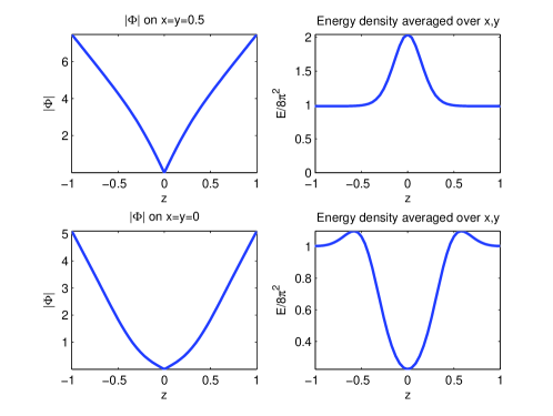
Figure 2: Higgs field and energy density of two double-wall solutions

The top row of Fig 2 illustrates a numerically-generated solution which is a non-infinitesimal version of the $C_{\alpha}=(0,0,1,0)$ case. The quantities plotted are the same as in Fig 1. The solution has $M_{+}=0.2$ and $D_{x}=D_{y}=1.8$. There is a double monopole (a torus with its axis in the $z$-direction) at $(x,y,z)=({\scriptstyle\frac{1}{2}},{\scriptstyle\frac{1}{2}},0)$, and this is where the energy density is peaked.

If, however, $C_{3}=C_{4}=0$, but $|C_{1}|^{2}+|C_{2}|^{2}\neq 0$ and hence $M_{+}<0$, then $\Phi$ is identically zero on $z=0$, whereas the energy density is minimal on $z=0$ and peaked off $z=0$. The bottom row of Fig 2 depicts a non-infinitesimal version of the $C_{\alpha}=(0,1,0,0)$ case, a solution having $M_{+}=-0.2$ and $D_{x}=D_{y}=-0.5$. The two solutions depicted in Fig 2 are Nahm transforms of each other, with their parameters and moduli being related as in (6, 7).

5 Geodesic surfaces, geodesics, and trajectories

One can identify several geodesics in ${\cal M}$ as fixed-point sets of discrete isometries, and this section describes a few of them, together with their interpretation as monopole-scattering trajectories. When the monopoles are well-localized, one may visualize such isometries in terms of their action on the two-monopole system viewed as a single rigid body, with three principal axes of inertia, as in the ${\mathbb{R}}^{3}$ case [3]. The line joining the two monopoles is called the (body-fixed) 3-axis, a head-on collision results in a torus whose axis is the 1-axis, and the 2-axis is the line along which the monopoles emerge after scattering.

Let $\tau_{0}$ denote rotation by $180^{\circ}$ in the $xy$-plane: in other words $\tau_{0}:(x,y)\mapsto(1-x,1-y)$. Then $\tau_{0}$ maps $(M_{+},p_{+},q_{+})$ to $(M_{+},-p_{+},-q_{+})$; so if we take $p_{+}=q_{+}=0$, as we shall do from now on, then $\tau_{0}$ is a symmetry of the system, preserving both the Bogomolny equation and the boundary conditions. Also, $\tau_{0}$ leaves the relative phase $\omega$ of two well-separated monopoles unchanged, and maps $(D_{x},D_{y})$ to $(\bar{D}_{x},\bar{D}_{y})$. It follows that the fixed-point set of $\tau_{0}$ is a 2-dimensional geodesic surface ${\cal S}$ in the moduli space ${\cal M}$.

The quantities $D_{x}$ and $D_{y}$ are real-valued on ${\cal S}$, and in the asymptotic region of the moduli space we have $|D_{x}|\approx|D_{y}|\gg 1$. So ${\cal S}$ has four asymptotic components, according to whether each of $D_{x}$ and $D_{y}$ is positive or negative. This corresponds to having two monopoles, well-separated in the $z$-direction, with the same $(x,y)$-location: namely one of the four possibilities $(0,0)$, $({\scriptstyle\frac{1}{2}},0)$, $(0,{\scriptstyle\frac{1}{2}})$ or $({\scriptstyle\frac{1}{2}},{\scriptstyle\frac{1}{2}})$. The 3-axis is in the $z$-direction, and the direction of the 1-axis in the $xy$-plane corresponds to the relative phase $\omega$, which is unrestricted. So each of the four asymptotic components is a cylinder, on which the coordinates are $M\gg 1$ and $\omega\in S^{1}$.

In order for a monopole pair to be invariant under $\tau_{0}$, its 1-axis must either be orthogonal to the $z$-axis (as in the asymptotic situation of the previous paragraph) or parallel to it; this gives two disjoint components of ${\cal S}$, namely ${\cal S}_{1}$ and ${\cal S}_{0}$ respectively. (The same sort of thing happens in the singly-periodic monopole-chain case [6]: in that case, ${\cal M}$ contains a surface for which the 1-axis is orthogonal to the periodic axis, plus two surfaces, isometric to each other, for which the 1-axis is along the periodic axis.) As we shall see below, the four asymptotic cylinders of ${\cal S}$ referred to above are the ends of the single component ${\cal S}_{1}$.

We now find geodesics in ${\cal S}_{1}$ and ${\cal S}_{0}$ by imposing additional symmetries. Two such isometries of ${\cal M}$ correspond to reflections in the $xy$-plane, namely

$$\tau_{1} : x\mapsto 1-x,\Phi\mapsto-\Phi,$$ (17)

$$\tau_{2} : x\mapsto y,y\mapsto x,\Phi\mapsto-\Phi.$$ (18)

Note that, on ${\cal S}$, $\tau_{1}$ is equivalent to the reflection $y\mapsto 1-y$, and $\tau_{2}$ is equivalent to $x\mapsto-y$, $y\mapsto-x$; so it is unnecessary to consider these reflections as well. In the asymptotic region, requiring invariance under $\tau_{1}$ or $\tau_{2}$ has the effect of restricting the direction of the 1-axis (the relative phase of the two monopoles), and gives us geodesics in ${\cal S}_{1}$. The $\tau_{1}$-invariant fields have their 1-axis in the $x$- or $y$-direction, while the $\tau_{2}$-invariant fields have their 1-axis along either $x=y$ or $x=-y$. So in each asymptotic cylinder of ${\cal S}_{1}$, we can identify four geodesics, and each of them can be traced as it passes through the interior of ${\cal S}_{1}$, using the analogous ${\mathbb{R}}^{3}$ scattering behaviour. (Here we are imagining that the monopoles remain well-localized throughout, which is the case if $M_{+}\gg 1$. In the $M_{+}\ll-1$ case, the moduli space and its geodesics are the same, via the Nahm transform, but the scattering interpretation is necessarily different.) For example, start on the asymptotic cylinder $D_{x}\approx D_{y}<0$ (monopoles on $x=y=0$), with the 1-axis in the $x$-direction. Then the two incoming monopoles merge at $x=y=z=0$, separate along the $y$-axis, re-merge at $(x,y,z)=(0,{\scriptstyle\frac{1}{2}},0)$, separate in the $z$-direction, and finally emerge in the asymptotic cylinder with $D_{x}>0$, $D_{y}<0$. Each pair of asymptotic cylinders is connected by a geodesic (either $\tau_{1}$- or $\tau_{2}$-invariant) in this way, and so they are the ends of the single component ${\cal S}_{1}$ of the surface ${\cal S}$, as mentioned previously.

The fate of generic geodesics starting in the asymptotic region of ${\cal S}_{1}$ is less clear, but it seems likely that (unlike in the example above) they never emerge: they get trapped in the central region of ${\cal S}_{1}$, and continue travelling around the $z=0$ torus.

Let us now turn to geodesics on the other component of ${\cal S}$, namely ${\cal S}_{0}$. As before, we first focus on the $M_{+}>0$ case, where the monopoles are localized. They are necessarly confined to the $z=0$ plane — the two walls coincide, and the monopole motion takes place entirely within this double wall. We can get a good picture by thinking of perturbations of the constant-energy solution, as described in the previous section. In particular, we take the subclass of perturbations given by $C_{1}=C_{2}=0$: these fields are invariant under the $180^{\circ}$ rotation $\tau_{0}$, and in effect give us the surface ${\cal S}_{0}$. We fix $|C_{3}|^{2}+|C_{4}|^{2}$ in order to fix $M_{+}>0$, and factor out by the phase (16), so ${\cal S}_{0}$ is a 2-sphere $S^{2}$ on which $\xi=C_{4}/C_{3}$ is a stereographic coordinate. Note, however, that the metric on ${\cal S}_{0}$ is not the standard 2-sphere metric.

Four points on this sphere, namely $\xi=0,\infty,1\mbox{ and }-1$, correspond to toroidal double-monopoles at $(x,y)=({\scriptstyle\frac{1}{2}},{\scriptstyle\frac{1}{2}}),(0,0),(0,{\scriptstyle\frac{1}{2}})\mbox{ and }({\scriptstyle\frac{1}{2}},0)$ respectively. The point $\xi={\mathrm{i}}$ corresponds to a pair of monopoles at $(x,y)=({\scriptstyle\frac{1}{4}},{\scriptstyle\frac{1}{4}})\mbox{ and }({\scriptstyle\frac{3}{4}},{\scriptstyle\frac{3}{4}})$, while $\xi=-{\mathrm{i}}$ corresponds to a pair of monopoles at $(x,y)=({\scriptstyle\frac{1}{4}},{\scriptstyle\frac{3}{4}})\mbox{ and }({\scriptstyle\frac{3}{4}},{\scriptstyle\frac{1}{4}})$. Imposing various additional symmetries then gives closed geodesics on ${\cal S}_{0}$. For example, invariance under $\tau_{1}$ gives a geodesic passing through $\xi=0,1,\infty\mbox{ and }-1$ in that order; whereas $\tau_{2}$-invariance gives a geodesic passing through $\xi=0,{\mathrm{i}},\infty\mbox{ and }-{\mathrm{i}}$. These correspond to closed trajectories in which the two monopoles repeatedly scatter at right angles within the periodic $xy$-plane, via the toroidal double-monopoles listed above.

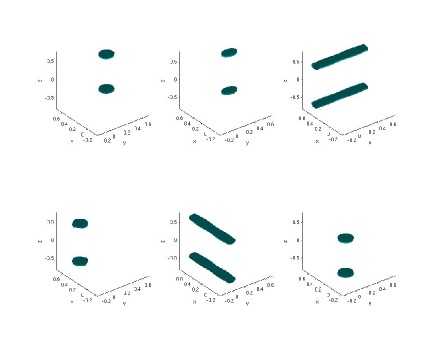
Figure 3: Part of a closed trajectory on ${\cal S}_{0}$ with $M_{+}<0$.

All this has a Nahm-transformed counterpart, with $M_{+}$ negative but close to zero. The fields are perturbations of the constant-energy solution (11) with $C_{3}=C_{4}=0$. Recall that the Higgs field is now identically zero on $z=0$, and that the energy density ${\cal E}$ is peaked off $z=0$. A geodesic can be visualized in terms of the movement of these energy peaks, and one such closed trajectory (or rather half of it) is illustrated in Fig 3. This shows six solutions, corresponding to six points on the curve $(C_{1},C_{2})=(\cos\eta,\sin\eta)$ for $0\leq\eta\leq\pi$, which is a closed geodesic in ${\cal S}_{0}$. Each of the figures is a 3-dimensional plot of the surface ${\cal E}(x,y,z)=0.95\max({\cal E})$, and so it indicates where the energy density is peaked. The upper-left figure shows peaks on $(x,y)=({\scriptstyle\frac{1}{2}},{\scriptstyle\frac{1}{2}})$. These elongate in the $y$-direction (top row), and re-localize as peaks on $(x,y)=({\scriptstyle\frac{1}{2}},0)$ (the lower-left figure). They then elongate in the $x$-direction before re-forming as peaks on $(x,y)=(0,0)$. The rest of the closed trajectory (not shown) then proceeds via peaks at $(x,y)=(0,{\scriptstyle\frac{1}{2}})$ before returning to the initial field.

6 Concluding remarks

In this paper, we have studied doubly-periodic BPS 2-monopole solutions, or double monopole walls. The moduli space of centred 2-monopole fields is a 4-dimensional manifold ${\cal M}$, and the moduli can be interpreted in terms of the relative monopole positions and phases. Even though the metric of ${\cal M}$ is not known explicitly (except in its asymptotic region), geodesics can be identified as fixed-point sets of discrete isometries, and these may be interpreted as the interaction of parallel monopole walls, or of the monopoles embedded in the walls.

For the gauge group SU(2), there are two topological charges $(Q_{-},Q_{+})$, and the number of monopoles is $N=Q_{-}+Q_{+}$. In this paper, we have only dealt with the charge $(1,1)$ case. For walls of charge $(0,2)$ or $(2,0)$, many of the details are similar, in particular the geometry of the moduli space. Rather less is currently known about $N>2$ solutions, and it would be interesting to investigate the existence of highly-symmetric multi-monopole-wall configurations along similar lines to the ${\mathbb{R}}^{3}$ case [3].

It would also be interesting to extend the analysis to the case of walls which have hexagonal rather than square symmetry. In particular, this would be relevant to the closely-related topic of monopole bags in ${\mathbb{R}}^{3}$ [13, 14, 15, 16, 17], which have curved hexagonal monopole walls separating their interior and exterior regions. It also motivates the question of the general dynamical behaviour of monopole walls, where double periodicity is not necessarily maintained, and so there are infinitely many degrees of freedom; little is currently known about this more general situation.

Acknowledgments. Both authors were supported by the UK Particle Science and Technology Facilities Council. For RSW this was through the Consolidated Grant No. ST/J000426/1.

References

- [1] N S Manton, A remark on the scattering of BPS monopoles. Physics Letters B 110 (1982) 54–56.
- [2] M F Atiyah and N J Hitchin, The geometry and dynamics of magnetic monopoles (Princeton University Press, Princeton, 1988).
- [3] N S Manton and P M Sutcliffe, Topological Solitons (Cambridge University Press, Cambridge, 2004).
- [4] S Cherkis and A Kapustin, Hyperkähler metrics from periodic monopoles. Physical Review D 65 (2002) 084015.
- [5] D Harland and R S Ward, Dynamics of periodic monopoles. Physics Letters B 675 (2009) 262–266.
- [6] R Maldonado and R S Ward, Geometry of periodic monopoles. Physical Review D 88 (2013) 125013.
- [7] R S Ward, Monopole wall. Physical Review D 75 (2007) 021701.
- [8] S A Cherkis and R S Ward, Moduli of monopole walls and amoebas. JHEP 1205(2012)090.
- [9] S A Cherkis, Phases of five-dimensional theories, monopole walls, and melting crystals. arXiv:1402.7117.
- [10] S A Cherkis, Instantons on gravitons. Commun Math Phys 306 (2011) 449–483.
- [11] M Hamanaka, H Kanno and D Muranaka, Hyperkähler metrics from monopole walls. Physical Review D 89 (2014) 065033.
- [12] F J W Olver, D W Lozier, R F Boisvert and C W Clark, NIST Handbook of Mathematical Functions (NIST and Cambridge University Press, Cambridge, 2010).
- [13] S Bolognesi, Multi-monopoles and magnetic bags. Nuclear Physics B 752 (2006) 93–123.
- [14] K-M Lee and E J Weinberg, BPS magnetic monopole bags. Physical Review D 79 (2009) 025013.
- [15] D Harland, The large limit of the Nahm transform. Commun Math Phys 311 (2012) 689–712.
- [16] D Harland, S Palmer and C Saemann, Magnetic Domains. JHEP 1210(2012)167.
- [17] C H Taubes, Magnetic bag like solutions to the SU(2) monopole equations on . arXiv:1302.5314