Search for Non-Standard Interactions by atmospheric neutrino

Abstract

We investigate the effects of neutral current Non-Standard Interactions in propagation on atmospheric neutrino experiments such as Super-Kamiokande and Hyper-Kamiokande. With the ansatz where the parameters which have strong constraints from other experiments are neglected, we show how these experiments put constraints on the remaining parameters of the Non-Standard Interactions.

1 Introduction

Neutrinos are the least tested particles of the Standard Model (SM). Furthermore non-zero neutrino masses, which cannot be explained by the SM, have been measured. Non-zero neutrino masses cause neutrino oscillation which may play an important role in searching for physics Beyond the Standard Model (BSM). All the three mixing angels in the standard three flavor neutrino oscillation have been measured by 2012. Tasks left for us are to measure the Dirac CP phase and the sign of $\Delta m^{2}_{31}$. It is expected that future high-intensity long-baseline experiments (T2HK,LBNO,LBNE etc.) may be able to measure these quantities and allow high precision measurement of the oscillation parameters. Hence the future experiments can take us to a new stage in which BSM is searched by looking at deviation from the SM with neutrino masses. For this reason, it is important to study new physics in neutrino sector.

2 New Physics

We consider flavor-dependent exotic couplings of neutrinos with matter in this talk. These Non-Standard Interactions (NSI) are divided into Charged-Current (CC) interactions and Neutral-Current(NC) interactions. We consider only non-standard NC interactions in propagation because constraints for non-standard CC interactions at detectors and sources are much stronger than those in propagation. They are expressed by effective 4-fermi interactions:

$${\cal L}_{NP}=-2{\sqrt{2}}G_{F}[\bar{\nu}_{\alpha}\gamma^{\mu}\nu_{\beta}][\epsilon_{\alpha\beta}^{f_{L}}\bar{f}_{L}\gamma_{\mu}f_{L}+\epsilon_{\alpha\beta}^{f_{R}}\bar{f}_{R}\gamma_{\mu}f_{R}],$$ (1)

where $\alpha,\beta$ are neutrino flavor indices and $\epsilon_{\alpha\beta}^{f_{L,R}}$ denotes the strength of the NSI between the neutrinos $\nu$ and left-handed (right-handed) components of the fermions $f$. It is known that neutrinos feel potentials as matter effects when they are propagating in matter. If NSI exist, neutrinos feel additional matter effects and the oscillation probability is modified significantly. NSI can be parameterized in the form of matter effects

$${\cal A}_{NSI}=A_{\rm CC}\left(\begin{array}[]{ccc}\epsilon_{ee}&\epsilon_{e\mu}&\epsilon_{e\tau}\\ \epsilon_{e\mu}^{*}&\epsilon_{\mu\mu}&\epsilon_{\mu\tau}\\ \epsilon_{e\tau}^{*}&\epsilon_{\mu\tau}^{*}&\epsilon_{\tau\tau}\\ \end{array}\right),$$ (2)

where

$$\epsilon_{\alpha\beta}=\sum_{P=L,R}\sum_{f=e,u,d}\epsilon^{f_{P}}_{\alpha\beta}n_{f}/n_{e}.$$ (3)

Here $n_{f}$ denotes number density of fermion $f$ and $A_{\rm CC}=\sqrt{2}G_{F}n_{e}$. In the case of atmospheric neutrino experiments, neutrinos go through the Earth, which is composed of protons($uud$), neutrons($udd$), and electrons and their number densities are approximately equal. Then we have

$$\epsilon_{\alpha\beta}\simeq\sum_{P=L,R}(\epsilon_{\alpha\beta}^{e_{P}}+3\epsilon_{\alpha\beta}^{u_{P}}+3\epsilon_{\alpha\beta}^{d_{P}}).$$ (4)

Matter effects affect the oscillation probability mainly when the baseline is longer and the neutrino energy is in the range $10{\rm GeV}<E<100{\rm GeV}$. Therefore atmospheric neutrino experiments such as Super-Kamiokande(SK) and Hyper-Kamiokande(HK) are suited to search for NSI.

3 Constraints on NSI

NSI are constrained by various experiments. For instance the most direct limits on $\epsilon_{\alpha\beta}$ are given by experiments of scattering of neutrino beams on target. This kind of experiments give constraints on each $\epsilon_{\alpha\beta}^{f_{L,R}}$ in (1), while the neutrino oscillation experiments can constrain the total sum $\epsilon_{\alpha\beta}$ in (4).

3.1 Constraints from terrestrial experiments

Constraints form terrestrial experiments are deduced as [1] :

$$\left(\begin{array}[]{lll}|\epsilon_{ee}|<4\times 10^{0}&|\epsilon_{e\mu}|<3\times 10^{-1}&|\epsilon_{e\tau}|<3\times 10^{0}\\ &|\epsilon_{\mu\mu}|<7\times 10^{-2}&|\epsilon_{\mu\tau}|<3\times 10^{-1}\\ &&|\epsilon_{\tau\tau}|<2\times 10^{1}\\ \end{array}\right).$$ (5)

The muon sector is strongly constrained, so we set $\epsilon_{e\mu},\epsilon_{\mu\mu},\epsilon_{\tau\mu}$ to zero in our analysis. On the other hand, the others are less constrained and hence there are rooms for improvement.

3.2 Constraints from the high energy behavior of atmospheric neutrino

The high energy atmospheric neutrino data are well described by vacuum oscillation between $\nu_{\mu}$ and $\nu_{\tau}$ but NSI can modify the oscillation probability significantly. Friedland-Lunardini [2] pointed out that large NSI are consistent with the data, provided that epsilons have the following relation:

$$\epsilon_{\tau\tau}\simeq\frac{|\epsilon_{e\tau}|^{2}}{1+\epsilon_{ee}}.$$ (6)

3.3 Summery of the constraints on NSI

Taking these constraints on NSI into consideration, we analyze with the following ansatz:

$$\left(\begin{array}[]{ccc}\epsilon_{ee}&\epsilon_{e\mu}&\epsilon_{e\tau}\\ \epsilon_{e\mu}^{*}&\epsilon_{\mu\mu}&\epsilon_{\mu\tau}\\ \epsilon_{e\tau}^{*}&\epsilon_{\mu\tau}^{*}&\epsilon_{\tau\tau}\\ \end{array}\right)=\left(\begin{array}[]{ccc}\epsilon_{ee}&0&|\epsilon_{e\tau}|e^{i\phi}\\ 0&0&0\\ |\epsilon_{e\tau}|e^{-i\phi}&0&\frac{|\epsilon_{e\tau}|^{2}}{1+\epsilon_{ee}}\\ \end{array}\right).\$$ (7)

Here $\phi$ is a phase of $\epsilon_{e\tau}$. Furthermore we introduce the following ratio:

$$|\tan\beta|\equiv\frac{|\epsilon_{e\tau}|}{1+\epsilon_{ee}}.$$ (8)

From the data of SK, Friedland-Lunardini [3] gave constraints $|\tan\beta|<1.5$ at 2.5$\sigma$ C.L. . What we want to do is to give an allowed region, which is obtained from SK or is expected from HK, in the $\epsilon_{ee}-|\epsilon_{e\tau}|$ plane.

4 Results

In our $\chi^{2}$ analysis, we fix the following oscillation parameters

$$\sin^{2}2\theta_{12}=0.86,\hskip 11.38092pt\sin^{2}2\theta_{13}=0.1,\hskip 11.38092pt\Delta m^{2}_{21}=7.6\times 10^{-5}{\rm eV},$$ (9)

while taking $\theta_{23}$, $\Delta m^{2}_{31}$, $\delta_{CP}$ and $\phi$ as free. To obtain a 2-dimensional allowed region, $\chi^{2}$ is marginalized over $\theta_{23}$, $\Delta m^{2}_{31}$, $\delta_{CP}$, $\phi$. In the case of SK, we look at difference of significance from the SK data. In the case of HK, we look at difference of significance from the standard case which is predicted with the standard oscillation parameters in our calculation code. The numbers of events of atmospheric neutrinos are calculated based on Ref. [7].

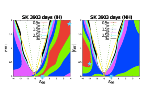
Figure 1: Constraints on NSI at SK with NH(right) and IH(left). Dotted lines denote constraints on $|\tan\beta|<1.5$ given by Friedland-Lunardini in 2005. Solid lines are our results($|\tan\beta|<0.8$). These lines are drawn at $2.5\sigma$ C.L. Stars are best fit points and double circles denote standard case($\epsilon_{\alpha\beta}=0$).

Figure 1 shows constraints on NSI from SK. Although updated data of SK (3903 days) are used, large NSI are not excluded. In addition, the standard case is not the best fit. The reason that a scenario with new physics is preferred may be because we have not reproduced SK MC results completely. However, the excluded region is improved compared with the old one given by Friedland-Lunardini in 2005. Figure 2 shows constraints on NSI at HK.

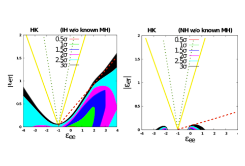
Figure 2: Constraints on NSI at HK with NH(right) and IH(left). They are drawn without knowledge of mass hierarchy. The dotted and solid lines are as with fig.1 and dashed lines are constraints on NSI at HK. In the case of NH($|\tan\beta|<0.06$) and IH($|\tan\beta|<0.3$).

The excluded region from HK is improved compared with SK and the region $|\epsilon_{e\tau}|>1$ is excluded. Finally figure 3 shows sensitivity to the non-zero NSI parameters at HK(90% C.L.). In the presence of new physics, HK can determine NSI to some extent with 90% C.L.. The results at HK are first obtained in this work.

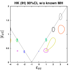
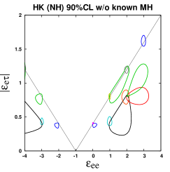
Figure 3: Sensitivity to non-zero NSI parameters at HK(90% C.L.)

5 Conclusion

Taking into consideration the constraints from the terrestrial experiments and the high energy behavior of atmospheric neutrinos, i.e., with the ansatz : $\epsilon_{e\mu}=\epsilon_{\mu\mu}=\epsilon_{\mu\tau}=0$ and $\epsilon_{\tau\tau}=|\epsilon_{e\tau}|^{2}/(1+\epsilon_{ee})$, we have searched for NSI. Under the ansatz we studied sensitivity to NIS of $\nu_{e}-\nu_{\tau}$ sector in propagation at SK and HK. Then the excluded region at SK is improved compared with the old one given by Friedland-Lunardini in 2005, because we used the updated SK data. The excluded region expected at HK is obtained and HK is expected to improve constraints. In addition we studied sensitivity to non-zero NSI parameters at HK. If NSI are sufficiently large, HK can determine $\epsilon_{ee}$ and $|\epsilon_{e\tau}|$ to some extent.

References

References

- [1] C. Biggio, M. Blennow and E. Fernandez-Martinez, JHEP 0908 (2009) 090 [arXiv:0907.0097 [hep-ph]].
- [2] A. Friedland, C. Lunardini, and M. Maltoni, Phys. Rev. D 70, 111301(R) (2004) [arXiv:hep-ph/0408264].
- [3] A. Friedland and C. Lunardini, Phys. Rev. D 72, 053009 (2005) [arXiv:hep-ph/0506143].
- [4] M. C. Gonzalez-Garcia, M. Maltoni and J. Salvado, JHEP 1105 (2011) 075 [arXiv:1103.4365 [hep-ph]].
- [5] G. Mitsuka et al. [Super-Kamiokande Collaboration], Phys. Rev. D 84, 113008 (2011) [arXiv:1109.1889 [hep-ex]].
- [6] M. C. Gonzalez-Garcia and M. Maltoni, JHEP 1309 (2013) 152 [arXiv:1307.3092].
- [7] O. Yasuda, Phys. Rev. D 58, 091301(R) (1998) [arXiv:hep-ph/9804400].