Coxeter-Knuth graphs and a signed Little map
for type $B$ reduced words

Abstract.

We define an analog of David Little’s algorithm for reduced words in type B, and investigate its main properties. In particular, we show that our algorithm preserves the recording tableaux of Kraśkiewicz insertion, and that it provides a bijective realization of the type B transition equations in Schubert calculus. Many other aspects of type A theory carry over to this new setting. Our primary tool is a shifted version of the dual equivalence graphs defined by Assaf and further developed by Roberts. We provide an axiomatic characterization of shifted dual equivalence graphs, and use them to prove a structure theorem for the graph of type B Coxeter-Knuth relations.

1. Introduction

Stanley symmetric functions $F_{w}$ appear in the study of reduced words of permutations [32], the representation theory of generalized Specht modules [19], and the geometry of positroid varieties [17]. The $F_{w}$ are known to have a Schur positive expansion with coefficients determined by the Edelman-Greene correspondence. This correspondence associates to each reduced word a pair of tableaux $(P,Q)$ of the same shape where the second tableau is standard. These symmetric functions $F_{w}$ can be defined as the sum of certain fundamental quasisymmetric functions where the sum is over all reduced words for $w\in S_{n}$, denoted $R(w)$. In particular, the coefficient of $x_{1}x_{2}\cdots x_{\ell(w)}$ in $F_{w}$ equals $|R(w)|$. There is a recurrence relation for $F_{w}$ derived from Lascoux and Schützenberger’s transition equation for Schubert polynomials [23] of the form

$$F_{w}=\sum_{w^{\prime}\in T(w)}F_{w^{\prime}},$$

along with the base cases that $F_{w}$ is a single Schur function if $w$ has at most one descent; in this case we say $w$ is Grassmannian. By taking the coefficient of $x_{1}x_{2}\cdots x_{\ell(w)}$ on both sides of the recurrence, we see that the sets $R(w)$ and $\cup_{w^{\prime}\in T(w)}R(w^{\prime})$ are equinumerous.

David Little gave a remarkable bijection between $R(w)$ and $\cup_{w^{\prime}\in T(w)}R(w^{\prime})$ [25] inspired by the lectures of Adriano Garsia, which are published as a book [12] . This algorithm is a finite sequence of steps, each of which decrements one letter in the word. If ever a 1 is decremented to a 0, then instead the whole reduced word is lifted up by one to make space for one extra generator. This bijection is an instance of a more general phenomenon known as Little bumps.

Recently, Hamaker and Young [16] have shown that Little bumps preserve the recording tableaux under the Edelman-Greene correspondence. This proved a conjecture of Thomas Lam [20, Conj. 2.5]. They further show that all reduced words with a given recording tableau $Q$ under the Edelman-Greene correspondence are connected via Little bumps. Edelman and Greene gave a refinement on the Coxeter relations in type $A$, which they call Coxeter-Knuth relations. These relations preserve the insertion tableaux under the Edelman-Greene correspondence, and the set of reduced words which have a fixed insertion tableau $P$ is connected by elementary Coxeter-Knuth relations. Hamaker and Young further showed that two reduced words that differ by an elementary Coxeter-Knuth relation give rise to $Q$ tableaux that differ in exactly two positions. This can be made more precise. Consider the graph $CK_{A}(w)$ on all reduced words for $w$ with an edge labeled $i$ between two reduced words $a=a_{1}a_{2}\cdots a_{p}$ and $b=b_{1}b_{2}\cdots b_{p}$ whenever $a$ and $b$ differ by an elementary Coxeter-Knuth relation in positions $i,i+1,i+2$. Call $CK_{A}(w)$ a Coxeter-Knuth graph. Using the theory of dual equivalence graphs due to Assaf [3] and the equivalent axioms given by Roberts [27], one can easily show that $CK_{A}(w)$ is a dual equivalence graph and the $Q$ tableaux for two reduced words differing by an elementary Coxeter-Knuth move differ by one of Haiman’s dual equivalence moves [15].

In this paper, we define the analog of the Little bump $B^{\delta}_{(i,j)}$ on reduced words for the signed permutations $B_{n}$, and show that these maps satisfy many of the same properties as in the original case. The superscript $\delta\in\{+,-\}$ denotes the direction of the bump, and the subscript $(i,j)$ indicates the crossing where the bump begins. In particular, there is a close connection to the Stanley symmetric functions for types B and C defined in [6], see also [11, 22]. These Stanley symmetric functions again satisfy a transition equation [5], which proves that $R(w)$ is equinumerous with a certain union of $R(w^{\prime})$’s.

To concretely state our first main result, we need to establish some notation. A signed permutation $w\in B_{n}$ is a bijection from $\{-n,\dots-1,1,2,\dots,n\}$ to itself such that $w(i)=-w(-i)$. One could represent $w$ in one-line notation either by listing $[w(-n),w(-n+1),\dots,w(-1),w(1),\dots,w(n)]$ in long form or simply $[w(1),\dots,w(n)]$ in short form. For example, $[1,\bar{2},\bar{4},3,\bar{3},4,2,\bar{1}]$ and $[\bar{3},4,2,\bar{1}]$ represent the same element in $B_{4}$ where $-i$ is denoted $\bar{i}$. For our purposes, we identify $v\in B_{n}$ with the element $w\in B_{n+1}$ such that $v(i)=w(i)$ for $1\leq i\leq n$ and $w(n+1)=n+1$. Set $B_{\infty}=\cup B_{n}$ in this identification. For $i<j\in\mathbb{Z}\setminus\{0\}$, let $t_{ij}$ be the (signed) transposition such that $t_{ij}(i)=j$, $t_{ij}(j)=i$, $t_{ij}(-i)=-j$, $t_{ij}(-j)=-i$ and for every integer $k\not\in\{\pm i,\pm j,0\}$ we have $t_{ij}(k)=k$. If $w\in B_{\infty}$ has $w(1)<w(2)<\dots$, we say $w$ is increasing. If $w$ is not increasing, let $(r<s)$ be the lexicographically largest pair of positive integers such that $w_{r}>w_{s}$. Set $v=wt_{rs}$. Let $T(w)$ be the set of all signed permutations $w^{\prime}=vt_{ir}$ for $i<r,i\neq 0$ such that $\ell(w^{\prime})=\ell(w)$.

Theorem 1.1.

Using the notation above, if $w\in B_{\infty}$ is not increasing, then the particular Little bump $B^{-}_{(r,s)}\ :\ R(w)\longrightarrow\bigcup_{w^{\prime}\in T(w)}R(w^{\prime})$ is the bijection predicted by the transition equation for type C Stanley symmetric functions.

The analog of Edelman-Greene insertion and elementary Coxeter-Knuth relations for signed permutations were given by Kraśkiewicz [18]. Kraśkiewicz insertion inputs a reduced word $a$ and outputs two shifted tableaux $(P^{\prime}(a),Q^{\prime}(a))$ of the same shifted shape where the recording tableau $Q^{\prime}(a)$ is standard. We develop some properties of the signed Little bumps and the recording tableaux as maps on reduced words summarized in the next theorem.

Theorem 1.2.

Suppose $w$ and $wt_{ij}$ are signed permutations such that $\ell(w)=\ell(wt_{ij})+1$.

1. The Little bump $B^{\delta}_{(i,j)}$ maps $R(w)$ to reduced words for some signed permutation $w^{\prime}=wt_{ij}t_{kl}$ with $\ell(w)=\ell(w^{\prime})$.

2. Two reduced words $a$ and $b$ are connected via Little bumps if and only if $Q^{\prime}(a)=Q^{\prime}(b)$ under Kraśkiewicz insertion.

3. For each standard shifted tableau $Q^{\prime}$, there exists a unique reduced word $a$ for an increasing signed permutation such that $Q^{\prime}(a)=Q^{\prime}$.

The Coxeter-Knuth relations given by Kraśkiewicz lead to a type B Coxeter-Knuth graph $CK_{B}(w)$ for each $w\in B_{\infty}$. An important step in proving Theorem 1.2 is showing that two reduced words for signed permutations that differ by an elementary Coxeter-Knuth relation give rise to two $Q^{\prime}$ tableaux that differ by one of Haiman’s shifted dual equivalence moves [15]. In fact, shifted dual equivalence completely determines the graph structure for type B Coxeter-Knuth graphs and vice versa. Thus, we define shifted dual equivalence graphs in analogy with the work of Assaf and Roberts on dual equivalence graphs.

Theorem 1.3.

Every type B Coxeter-Knuth graph $CK_{B}(w)$ is a shifted dual equivalence graph with signature function given via peak sets of reduced words. The isomorphism is given by $Q^{\prime}$ in Kraśkiewicz insertion. Conversely, every connected shifted dual equivalence graph is isomorphic to the Coxeter-Knuth graph for some increasing signed permutation.

Putting Theorem 1.2 and Theorem 1.3 together, one can see that Little bumps in both type A and type B play a similar role for Stanley symmetric functions as jeu de taquin plays in the study of Littlewood-Richardson coefficients for skew-Schur functions. In particular, let us say that words $a$, $a^{\prime}$ communicate if there is a sequence of Little bumps which transforms $a$ into $a^{\prime}$. We will show that there is exactly one reduced word for a unique increasing signed permutation in each communication class under Little bumps.

We give local axioms characterizing graphs isomorphic to shifted dual equivalence graphs or equivalently Coxeter-Knuth graphs of type B. We state the theorem here using some terminology that is developed in Section 5.

Theorem 1.4.

A signed colored graph $\mathcal{G}=(V,\sigma,E)$ of shifted degree $[n]$ is a shifted dual equivalence graph if and only if the following local properties hold.

1. If $I$ is any interval of integers with $|I|\leq 9$, then each component of $\mathcal{G}|_{I}$ is isomorphic to the standard shifted dual equivalence graph of a shifted shape of size up to $|I|$.

2. If $i,j\in\mathbb{N}$ with $|i-j|>3$, $(u,v)\in E_{i}$ and $(u,w)\in E_{j}$, then there exists a vertex $y\in V(\mathcal{G})$ such that $(v,y)\in E_{j}$ and $(w,y)\in E_{i}$.

We propose that the study of Coxeter-Knuth graphs initiated in this paper is an interesting way to generalize dual equivalence graphs to other Coxeter group types. For example, in type $A$, dual equivalence graphs have been shown to be related to crystal graphs [2]. Furthermore, the transition equation due to Lascoux and Schützenberger follows from Monk’s formula for multiplying a special Schubert class of codimension 1 with an arbitrary Schubert class in the flag manifold of type $A$. The elementary Coxeter-Knuth relations could have been derived from the Little bijection provided one understood the Coxeter-Knuth relations for the base case of the transition equations in terms of Grassmannian permutations. The transition equations for the other classical groups follow from Chevalley’s generalization for Monk’s formula on Schubert classes [8]. In fact, there is a very general Chevalley Formula for all Kac-Moody groups [24].

We comment on one generalization which did not work as hoped. In type $A$, Chmutov showed that the molecules defined by Stembridge’s axioms can be given edge labels in such a way that the graphs are dual equivalence graphs [9]. Alas, in type B, this does not appear to be possible. The Kazhdan-Lusztig graph for $B_{3}$ has a connected component with an isomorphism type that does not occur for dual equivalence graphs or shifted dual equivalence graphs. Namely, the component of $[2,1,\bar{3}]$ is a tree with 4 vertices and 3 leaves $[1,\bar{2},\bar{3}],[\bar{2},\bar{3},1],[2,1,\bar{3}]$.

The paper proceeds as follows. In Section 2, we review the necessary background on permutations and signed permutations as Coxeter groups. In Section 3, we formally define the signed Little bumps and pushes. The key tool we use to visualize the algorithms is the wiring diagram of a reduced word. The conclusion of the proof of Theorem 1.1 is given in Corollary 3.9, and Theorem 1.2(1) follows directly from Theorem 3.7. The relationships between Little bumps, the recording tableaux under the Kraśkiewicz insertion, Coxeter-Knuth moves of type B and shifted dual equivalence moves are discussed in Section 4. The main results of this section prove Theorem 1.2, parts (2) and (3). In Section 5, the shifted dual equivalence graphs are equivalently defined in terms of either shifted dual equivalence moves or Coxeter-Knuth moves proving Theorem 1.3. Theorem 1.3 is an easy consequence of this definition and the machinary built up in Sections 2 and 4. We go on to prove many lemmas leading up to the axiomatization of shifted dual equivalence graphs proving Theorem 1.4. We conclude with some interesting open problems in Section 6.

We recently learned that Assaf has independently considered shifted dual equivalence graphs in connection to a new Schur positive expansion of the Schur $P$-polynomials [1]. In particular, the connection between shifted dual equivalence graphs and Little bumps is new to this article.

2. Background

Let $W$ be a Coxeter group with generators $S=\{s_{1},\ldots,s_{n}\}$ and elementary relations $\left(s_{i}s_{j}\right)^{m(i,j)}=1$. For $w\in W$, let $\ell(w)$ be the minimal length of any expression $s_{a_{1}}\cdots s_{a_{q}}=w$. If $\ell(w)=p$, we say $s_{a_{1}}\cdots s_{a_{p}}$ is a reduced expression and the list of subscripts $a_{1}a_{2}\cdots a_{p}$ is a reduced word for $w=s_{a_{1}}s_{a_{2}}\cdots s_{a_{p}}$. Let $R(w)$ be the set of reduced words for $w$.

For $w\in W$, one can define a graph $G(w)$ with vertices given by the reduced words of $w$ using the Coxeter relations. In this graph, any two reduced words are connected by an edge if they differ only by an elementary relation of the form $s_{i}s_{j}s_{i}\cdots=s_{j}s_{i}s_{j}\cdots$ where each side is a product of $m(i,j)$ generators. It is a well known theorem, sometimes attributed to Tits, that this graph is connected [7, Thm. 3.3.1].

2.1. Type A

The symmetric group $S_{n}$ is the Coxeter group of type $A_{n-1}$. For our purposes, we can think of $w\in S_{n}$ in one-line notation as $w=[w_{1},w_{2},\ldots,w_{n}]$ or as $w=[w_{1},w_{2},\dots]\in S_{\infty}$ with $w_{i}=i$ for all $i>n$. Let $t_{ij}$ be the transposition interchanging $i$ and $j$ and fixing all other values. Then right multiplication by $t_{ij}$ interchanges the values in positions $i$ and $j$ in $w$.

The group $S_{n}$ is minimally generated by the adjacent transpositions $s_{1},\ldots,s_{n-1}$, where $s_{i}=t_{i,i+1}$, with elementary Coxeter relations

1. Commutation: $s_{i}s_{j}=s_{j}s_{i}$ provided $|i-j|>1$,

2. Braid: $s_{i}s_{i+1}s_{i}=s_{i+1}s_{i}s_{i+1}$.

For example, if $w=[2,1,5,4,3]$, then

$$R(w)=\{1343,3143,3413,3431,4341,4314,4134,1434\}$$

and $G(w)$ is a cycle on these 8 vertices.

In [10], Edelman-Greene (EG) gave an insertion algorithm much like the famous Robinson-Schensted-Knuth (RSK) algorithm for inserting a reduced word into a tableau for some partition $\lambda=(\lambda_{1}\geq\lambda_{2}\geq\ldots\geq\lambda_{k}>0)$. The one difference in EG insertion is that when inserting an $i$ into a row that already contains an $i$ and $i+1$, we skip that row and insert $i+1$ into the next row. If one keeps track of the recording tableau of the insertion, then the process is invertible. Let $P(a)$ be the EG insertion tableau for $a=a_{1}\dots a_{p}$ and let $Q(a)$ be the recording tableau. Define $EG(w)=\{P:P=P(a)\ \text{ for some }a\in R(w)\}$.

For example, using EG insertion, the reduced word $1343$ inserts to give aligntableaux=bottom, smalltableaux

$$\ytableaushort{1}\raisebox{2.58334pt}{ $\to$ }\ytableaushort{13}\raisebox{2.58334pt}{ $\to$ }\ytableaushort{134}\raisebox{2.58334pt}{ $\to$ }\ytableaushort{4,134}.$$

So

$$\ytableausetup{aligntableaux=center,smalltableaux}P(1343)=\ytableaushort{4,134}\hskip 21.68121pt\text{and}\hskip 21.68121ptQ(1343)=\ytableaushort{4,123}$$

in French notation.

The EG recording tableau $Q(a)$ is a standard Young tableau of partition shape $\lambda$, denoted $SYT(\lambda)$. These are bijective fillings of the Ferrers diagram for the partition $\lambda$ with rows and columns increasing. The row reading word of a standard tableau $T$ is the permutation in one-line notation obtained by reading along the rows of $T$ in the French way, left to right and top to bottom. The ascent set of $T$ is the set of all $i$ such that $i$ precedes $i+1$ in the row reading word of $T$. Similarly, define the ascent set of a reduced word $a=a_{1}\cdots a_{p}$ to be $\{j:a_{j}<a_{j+1}\}$. If a position is not an ascent, it is called a descent.

Theorem 2.1.

[10, Theorems 6.25 and 6.27] Fix $w\in S_{\infty}$ and $P\in EG(w)$. Then, the recording tableau for EG insertion gives a bijection between $\{a\in R(w):P(a)=P\}$ and the set of standard Young tableaux of the same shape as $P$. Furthermore, this bijection preserves ascent sets.

Definition 2.2.

Let $a_{\lambda,w}$ be the number of distinct tableaux $P\in EG(w)$ such that $P$ has shape $\lambda$. We call these numbers the Edelman-Greene coefficients.

Definition 2.3.

[32] For $w\in S_{\infty}$ and $a=a_{1}\cdots a_{p}\in R(w)$, let $I(a)$ be the set of all increasing integer sequences $1\leq i_{1}\leq i_{2}\leq\dotsb\leq i_{p}$ such that $i_{j}<i_{j+1}$ whenever $a_{j}<a_{j+1}$. The Stanley symmetric function $F_{w}=F^{A}_{w}$ is defined by

$$F^{A}_{w}=\sum_{a\in R(w)}\sum_{i_{1}i_{2}\dotsb i_{p}\in I(a)}x_{i_{1}}x_{i_{2}}\cdots x_{i_{p}}.$$

Here, the inner summation $\sum_{i_{1}i_{2}\dotsb i_{p}\in I(a)}x_{i_{1}}x_{i_{2}}\cdots x_{i_{p}}$ is the fundamental quasisymmetric function indexed by the ascent set of $a$ [31, Ch. 7.19]. Edelman-Greene showed that the ascent set of $a\in R(w)$ agrees with the ascent set of $Q(a)$. Furthermore, Ira Gessel [13] showed that the Schur function $s_{\lambda}$ is the sum over all standard tableaux $T$ of shape $\lambda$ of the fundamental quasisymmetric function by the ascent set of $T$. Putting this together gives the following theorem.

Theorem 2.4.

[10, Theorem 6.27] Fix $w\in S_{\infty}$. Then

$$F^{A}_{w}=\sum_{\lambda}a_{\lambda^{\prime},w}s_{\lambda},$$

where $s_{\lambda}$ is the Schur function indexed by the partition $\lambda$, $\lambda^{\prime}$ is the conjugate partition obtained from $\lambda$ by counting the length of the columns in the Ferrers diagram, and each $a_{\lambda^{\prime},w}$ is a nonnegative integer given in Definition 2.2.

Edelman-Greene also characterized when two reduced expressions give rise to the same $P$ tableau by restricting the elementary Coxeter relations. For this characterization, they define the elementary Coxeter-Knuth relations to be either a braid move or a witnessed commutation move:

1. $ikj\leftrightarrow kij$ for all $i<j<k$,

2. $jik\leftrightarrow jki$ for all $i<j<k$,

3. $i(i+1)i\leftrightarrow(i+1)i(i+1)$.

Two words which are connected via a sequence of Coxeter-Knuth relations are said to be in the same Coxeter-Knuth class.

Theorem 2.5.

[10, Theorem 6.24] Let $a,b\in R(w)$. Then $P(a)=P(b)$ if and only if $a$ and $b$ are in the same Coxeter-Knuth class.

In the example $w=[2,1,5,4,3]$, there are three Coxeter-Knuth classes $\{3143,3413\}$, $\{3431,4341,4314\}$, and $\{1343,4134,1434\}$, which respectively insert to the three $P$ tableaux:

$$\ytableausetup{aligntableaux=bottom,smalltableaux}\ytableaushort{34,13}\hskip 14.45377pt\ytableaushort{4,3,14}\hskip 14.45377pt\ytableaushort{4,134}.$$

Let $CK_{A}(w)$ be the Coxeter-Knuth graph for $w\in S_{\infty}$ with vertices $R(w)$ and colored (labeled) edges constructed using Coxeter-Knuth relations. An edge between $a$ and $b$ is labeled $i$ if $a_{j}=b_{j}$ for all $j\not\in\{i,i+1,i+2\}$ and $a_{i}a_{i+1}a_{i+2}$ and $b_{i}b_{i+1}b_{i+2}$ differ by an elementary Coxeter-Knuth relation. To each vertex $a\in R(w)$ associate a signature determined by its ascent set, $\sigma(a)=\{j:a_{j}<a_{j+1}\}$. If $\ell(w)=p$, we denote a subset $S\subset\{1,\ldots,p-1\}$ by a sequence in $\{+,-\}^{p-1}$ where $+$ in the $j^{th}$ position means $j\in S$. Here $\sigma_{j}(a)=+$ if $a_{j}<a_{j+1}$ and $\sigma_{j}(a)=-$ if $a_{j}>a_{j+1}$. See Figure 1 for an example and compare to $G(21543)$, which is a cycle with eight vertices, as mentioned above.

aligntableaux=center, smalltableaux

Figure 1. The Coxeter-Knuth graph of $w=[2,1,5,4,3]$.

Let $\alpha_{i}$ be the involution defined by the edges of $CK_{A}(w)$, namely $\alpha_{i}(a)=b$ provided $a$ and $b$ are connected by an edge colored $i$, or equivalently an elementary Coxeter-Knuth relation on positions $i,i+1,i+2$. If $a$ is not contained in an $i$-edge, then define $\alpha_{i}(a)=a$.

The type $A$ Coxeter-Knuth graphs are closely related to dual equivalence graphs on standard tableaux as defined by Assaf [3]. For a partition $\lambda$, one defines a standard dual equivalence graph $\mathcal{G}_{\lambda}$ to be the graph with vertex set given by $SYT(\lambda)$, and an edge colored $i$ between any two tableaux that differ by an elementary dual equivalence defined as follows.

Definition 2.6.

[15] Given a permutation $\pi\in S_{n}$, define the elementary dual equivalence operator $d_{i}$ for all $1\leq i\leq n-2$ as follows. Say $\{i,i+1,i+2\}$ occur in positions $a<b<c$ in $\pi$, then $d_{i}(\pi)=\pi t_{ac}$ provided $\pi(b)\neq i+1$ and $d_{i}(\pi)=\pi$ otherwise. Dual equivalence operators also act on standard tableaux by acting on their row reading word.

It was observed by the first author that the following theorem holds by combining the work in the original version of [16] and [27]. This was the start of our collaboration.

Theorem 2.7.

[16, Thm. 1.3] The graph $CK_{A}(w)$ is isomorphic to a disjoint union of standard dual equivalence graphs for each $w\in S_{n}$. The isomorphism preserves ascent sets on vertices. On each connected component, the Edelman-Green $Q$ function provides the necessary isomorphism. Furthermore, ascent sets are preserved.

2.2. Type B/C

The hyperoctahedral group, or signed permutation group $B_{n}$ is also a finite Coxeter group. This group is the Weyl group of both the root systems of types B and C of rank $n$. Recall from Section 1 that we have defined the (signed) transposition $t_{ij}$ to be the signed permutation interchanging $i$ with $j$ and $-i$ with $-j$ for all $i,j\neq 0$. The group $B_{n}$ is generated as a Coxeter group by the adjacent transpositions $s_{1},\ldots,s_{n-1}$ with $s_{i}=t_{i,i+1}$ plus an additional generator $s_{0}=t_{-1,1}$. Thus, if $w=[w_{1},\dots,w_{n}]\in B_{n}$, then $ws_{0}=[-w_{1},w_{2},\ldots,w_{n}]$. For example, $[\bar{3},2,1]=s_{1}s_{2}s_{1}s_{0}\in B_{3}$. Again, let $R(w)$ denote the set of all reduced words for $w$. Note that if $w\in S_{n}$, then it can also be considered as an element in $B_{n}$ with the same reduced words. The elementary relations on the generators are given by

1. Commutation: $s_{i}s_{j}=s_{j}s_{i}$ provided $|i-j|>1$,

2. Short Braid: $s_{i}s_{i+1}s_{i}=s_{i+1}s_{i}s_{i+1}$ for all $i>0$,

3. Long Braid: $s_{0}s_{1}s_{0}s_{1}=s_{1}s_{0}s_{1}s_{0}$.

Shifted tableaux play the same role in types B/C as the usual tableaux play in type $A$. Given a strict partition $\lambda=(\lambda_{1}>\lambda_{2}>\dotsb>\lambda_{k}>0)$, the shifted shape $\lambda$ is the set of squares in positions $\{(i,j)\ :\ 1\leq i\leq k,i\leq j\leq\lambda_{i}+i-1\}$. A standard shifted tableau $T$ is a bijective filling of a shifted shape with positive integers with rows and columns increasing. For example, see $T$ in Figure 2. Let $SST(\lambda)$ be the set of standard shifted tableaux of shifted shape $\lambda$.

aligntableaux=bottom S= 7
5&68
12349 ,         T= &7
368
12459 ,         U = &0
210
32101

Figure 2. A standard tableau $S$, standard shifted tableau $T$ and unimodal tableau $U$ respectively of shape $\lambda=(5,3,1)$.

We will also need to consider another type of tableaux on shifted shapes. We say a list $r=r_{1}\dots r_{l}$ is unimodal if there exists an index $j$, referred to as the middle, such that $r_{1}\dots r_{j}$ is decreasing and $r_{j}\dots r_{l}$ is increasing. A unimodal tableau $T$ is a filling of a shifted shape with nonnegative integers such that the reading word along each row is unimodal.

In 1989, Kraśkiewicz[18] gave an analog of Edelman-Greene insertion for reduced words of signed permutations. Kraśkiewicz insertion is a variant of the mixed shifted insertion of [14] that maps a reduced word $b$ of a signed permutation to the pair of shifted tableaux $(P^{\prime}(b),Q^{\prime}(b))$ where $Q^{\prime}(b)$ is a standard shifted tableau and $P^{\prime}(b)$ is a unimodal tableau of the same shape such that the reading word given by reading rows left to right from top to bottom is a reduced word for $w$. Once again, there is an analog of the Coxeter-Knuth relations. We will need the details of this insertion map and relations for our main theorems. Our description of this map is based on an equivalent algorithm in Tao Kai Lam’s Ph.D. thesis [22].

First, there is an algorithm to insert a non-negative integer into a unimodal sequence. Given a number $k$ and a (potentially empty) unimodal sequence $r=r_{1}\dots r_{l}$ with middle index $j$, we insert $k$ into $r$ and obtain another unimodal sequence as follows:

1. If $k\neq 0$ or $r_{j}\neq 0$, perform Edelman-Greene insertion of $k$ into $r_{j+1}\dots r_{l}$. Call the bumped entry $k^{-}$, if it exists. Call the resulting string after insertion $v_{1}\dots v_{q}$. Note, $q$ may be $l-j$ or $l-j+1$.

2. If $k=0$ and $r_{j}=0$, set $k^{-}=1$. Set $v_{1}\dots v_{q}=r_{j+1}\dots r_{l}$.

3. If $k^{-}$ exists, perform Edelman-Greene insertion of $-k^{-}$ into $-r_{1}\dots-r_{j}$. This time a bumped entry $-r_{i}$ will exist, as $k^{-}>r_{j}$. Set $k^{\prime}=r_{i}$. Set $u_{1}\dots u_{j}$ to be the result of negating every entry in the resulting string after insertion and reversing it.

4. If $k^{-}$ does not exist, set $u_{1}\dots u_{j}=r_{1}\dots r_{j}$.

5. Output the unimodal sequence $u_{1}\dots u_{j}v_{1}\dots v_{q}$ and $k^{\prime}$ if it exists.

The Kraśkiewicz insertion of a non-negative integer $k$ into a shifted unimodal tableau $P^{\prime}$ starts by inserting $k$ into the first row of $P^{\prime}$ using the algorithm above. Replace the first row of $P^{\prime}$ by $u_{1}\dots u_{p}v_{1}\dots v_{q}$. If $k^{-}$ exists and $k^{\prime}$ is the output, then insert $k^{\prime}$ in the second row of $P^{\prime}$, etc. Continue until no output exists or no further rows of $P^{\prime}$ exist. In that case, add $k^{\prime}$ in a new final row along the diagonal so the result is again a shifted unimodal tableau. Call the final tableau $P^{\prime}\leftarrow k$. For $w\in B_{\infty}$ and $a=a_{1}\dotsb a_{p}\in R(w)$, let $P^{\prime}(w)$ be the result of inserting $\emptyset\leftarrow a_{1}\dotsb a_{p}$ consecutively into the empty shifted unimodal tableau denoted $\emptyset$.

For example, using Kraśkiewicz insertion, on the same reduced word $1343$ as before inserts to give aligntableaux=bottom, smalltableaux

$$\ytableaushort{1}\raisebox{2.58334pt}{ $\to$ }\ytableaushort{13}\raisebox{2.58334pt}{ $\to$ }\ytableaushort{134}\raisebox{2.58334pt}{ $\to$ }\ytableaushort{\none 1,434}.$$

So

$$\ytableausetup{aligntableaux=bottom,smalltableaux}P^{\prime}(1343)=\ytableaushort{\none 1,434}\hskip 21.68121pt\text{and}\hskip 21.68121ptQ^{\prime}(1343)=\ytableaushort{\none 4,123}.$$

Also, $021032101\in R([\bar{3},\bar{4},\bar{1},2])$ gives $P^{\prime}=U,Q^{\prime}=T$ from Figure 2.

Kraśkiewicz insertion behaves well with respect to the peaks of a reduced word. Given any word $a_{1}\dots a_{p}$, we say $a$ has an ascent in position $0<i<p$ if $a_{i}<a_{i+1}$ and a descent if $a_{i}>a_{i+1}$. Similarly, we say $a$ has a peak in position $1<i<p$ if $a_{i-1}<a_{i}>a_{i+1}$. Define the peak set of $a\in R(w)$ to be $peaks(a)=\{1<i<p\ :\ a_{i-1}<a_{i}>a_{i+1}\}$. For example, $peaks(4565)=\{3\}$ and $peaks(7267)=\emptyset$. Recall that standard tableaux have associated ascent sets and descent sets as well as defined just before Theorem LABEL:edelman1987balanced. Given a standard (shifted) tableau $T$, we say $j$ is a peak of $T$ provided $j$ appears after $j-1$ and $j+1$ in the row reading word of $T$, so there is an ascent from $j-1$ to $j$ and a descent from $j$ to $j+1$. The peak set of $T$, denoted again $peaks(T)$, is defined similarly.

Theorem 2.8.

[22, Theorem 2.10] Given a signed permutation $w$ and a reduced word $a\in R(w)$, $peaks(a)=peaks(Q^{\prime}(a))$.

One important tool for studying Kraśkiewicz insertion is a family of local transformations on words known as the type B Coxeter-Knuth moves. These moves are based on certain type B elementary Coxeter relations that depend on exactly four adjacent entries of a word.

Definition 2.9.

[18] The elementary Coxeter-Knuth moves of type B are given by the following rules on any reduced word $i_{1}i_{2}i_{3}i_{4}$. If $i_{1}i_{2}i_{3}i_{4}$ has no peak then $\beta(i_{1}i_{2}i_{3}i_{4})=i_{1}i_{2}i_{3}i_{4}$. If $i_{1}i_{2}i_{3}i_{4}$ has a peak in position $3$, $\beta(i_{1}i_{2}i_{3}i_{4})$ is given by reversing $\beta(i_{4}i_{3}i_{2}i_{1})$. If $i_{1}i_{2}i_{3}i_{4}$ has a peak in position 2, then we have three cases:

1. Long braid: If $i_{1}i_{2}i_{3}i_{4}=0101$, then define $\beta(0101)=1010$. Note $1010$ is another reduced word for the same signed permutation, and it has a peak in position 3.

2. Short braid witnessed by smaller value: If there are 3 distinct letters among $i_{1}i_{2}i_{3}i_{4}$ and there is a corresponding short braid relation specifically of the form $i_{1}i_{2}i_{3}i_{4}=a\ b+1\ b\ b+1$ or $b\ b+1\ b\ a$ for some $a<b$. Define

   (2.1) $$\beta(a\ b+1\ b\ b+1) =a\ b\ b+1\ b\text{ and }$$

   (2.2) $$\beta(b\ b+1\ b\ a) =b+1\ b\ b+1\ a.$$

   Again the sequence $\beta(i_{1}i_{2}i_{3}i_{4})$ has a peak in position 3 since $a<b$. Also, this word is another reduced word for the same signed permutation which differs by a short braid move.

3. Peak moving commutation: In all other cases,

   $$\beta(i_{1}i_{2}i_{3}i_{4})=(i_{1}i_{2}i_{3}i_{4})s_{j}$$

   for the smallest $j$ such that $(i_{1}i_{2}i_{3}i_{4})s_{j}$ is related to $i_{1}i_{2}i_{3}i_{4}$ by a commuting move and has peak in position 3. Here $s_{j}$ is the operator acting on the right by swapping positions $j$ and $j+1$.

Observe that $i_{1}i_{2}i_{3}i_{4}$ is fixed by $\beta$ if and only if $i_{1}i_{2}i_{3}i_{4}$ has no peak. Furthermore, the map $\beta$ is an involution on $R(w)$ for $w$ a signed permutation with $\ell(w)=4$. Define a family of involutions $\beta_{i}$ acting on reduced words $a_{1}a_{2}\dotsb a_{p}$ by replacing $a_{i}a_{i+1}a_{i+2}a_{i+3}$ by $\beta(a_{i}a_{i+1}a_{i+2}a_{i+3})$,provided $0<i\leq p-3$.

Theorem 2.10.

[18] Let $a$ and $b$ be reduced words of signed permutations. Then $P^{\prime}(a)=P^{\prime}(b)$ if and only if there exist Coxeter-Knuth moves of type B relating $a$ to $b$. Furthermore, for each standard shifted tableau $Q$ of the same shape as $P^{\prime}(a)$, there exists a reduced word $c$ for the same signed permutation such that $P^{\prime}(c)=P^{\prime}(a)$ and $Q^{\prime}(c)=Q$.

Using the Coxeter-Knuth moves of type B, we can define an analogous graph $CK_{B}(w)$ on the reduced words for $w\in B_{n}$ with edges defined by the involutions $\beta_{i}$. Each connected component of $CK_{B}(w)$ has vertex set given by a Coxeter-Knuth equivalence class $\{a\in R(w)\ :\ P^{\prime}(a)=P^{\prime}\}$, and assuming this set is nonempty, $Q^{\prime}$ gives a bijection between this set and the standard shifted tableaux of the same shape as $P^{\prime}$. In Section 4, we will show that every connected component of $CK_{B}(w)$ is isomorphic to some $CK_{B}(v)$ where $v$ is increasing. In Section 5, we will show that $Q^{\prime}$ gives an isomorphism of signed colored graphs with a graph on standard shifted tableaux of the same shape with edges given by shifted dual equivalence.

2.3. Stanley symmetric functions revisited

For signed permutations, there are two forms of Stanley symmetric functions and their related Schubert polynomials, see [6, 11, 22]. The distinct forms correspond to the root systems of type B and C, which both have signed permutations as their Weyl group. The definition we will give is the type C version, from which the type B version can be readily obtained. First, we introduce an auxiliary family of quasisymmetric functions.

In type A, ascent sets of reduced words can be used to define the Stanley symmetric functions. In type B/C, the peak set of a reduced word plays a similar role.

Definition 2.11.

[6, Eq. (3.2)] Let $X=\{x_{1},x_{2},\dots\}$ be an alphabet of variables. The peak fundamental quasisymmetric function of degree $d$ on a possible peak set $P$ is defined by

$$\Theta_{P}^{d}(X)=\sum_{(i_{1}\leq\dots\leq i_{d})\in A_{d}(P)}2^{|\{i_{1},i_{2},\dots,i_{d}\}|}x_{i_{1}}x_{i_{2}}\cdots x_{i_{d}}$$

and $A_{d}(P)$ is the set of all admissible sequences $(1\leq i_{1}\leq\dots\leq i_{d})$ such that $i_{k-1}=i_{k}=i_{k+1}$ only occurs if $k\not\in P$.

The peak fundamental quasisymmetric functions also arise in Stembridge’s enumeration of $P$-partitions [33] and are a basis for the peak subalgebra of the quasisymmetric functions as studied by [4, 30] and many others. They are also related to the Schur $Q$-functions $Q_{\mu}(X)$ which are specializations of Hall-Littlewood polynomials $Q_{\mu}(X;t)$ with $t=-1$, see [26, III]. By [6, Prop. 3.2], the following is an equivalent definition of Schur $Q$-functions.

Definition 2.12.

For a shifted shape $\mu$, the Schur $Q$-function $Q_{\mu}(X)$ is

$$Q_{\mu}(X)=\sum_{T}\Theta_{peaks(T)}^{|\mu|}(X)$$

where the sum is over all standard shifted tableaux $T$ of shape $\mu$.

Remark 2.13.

In this way, the peak fundamental quasisymmetric functions play the role of the original fundamental quasisymmetric functions in Gessel’s expansion of Schur functions [13].

Let $g_{w}^{\mu}$ be the number of distinct shifted tableaux of shape $\mu$ that occur as $P^{\prime}(a)$ for some $a\in R(w)$ under Kraśkiewicz insertion. The numbers $g_{w}^{\mu}$ can equivalently be defined as the number of reduced words in $R(w)$ mapping to any fixed standard tableaux of shape $\mu$ by Haiman’s promotion operator [15, Prop. 6.1 and Thm. 6.3 ]. Haiman’s promotion operator on $a\in R(w)$ in type B is equivalent to Kraśkiewicz’s $Q^{\prime}(a)$. Recall from Theorem 2.8 that $Q^{\prime}(a)$ and $a$ have the same peak set which implies the equivalence in the following definition.

Definition 2.14.

[6, Prop. 3.4] For $w\in B_{\infty}$ with $d=\ell(w)$, define the type C Stanley symmetric function to be

$$F^{C}_{w}(X) =\sum_{\mu}g_{w}^{\mu}Q_{\mu}(X)$$

$$=\sum_{a\in R(w)}\Theta^{\ell(w)}_{peaks(a)}(X)$$

$$=\sum_{a\in R(w)}\hskip 7.22743pt\sum_{(i_{1}\leq\dots\leq i_{d})\in A_{d}(P)}2^{|\{i_{1},i_{2},\dots,i_{p}\}|}x_{i_{1}}x_{i_{2}}\cdots x_{i_{d}}.$$

Every Schur $Q$-function is itself a type C Stanley symmetric function. In particular, for the shifted partition $\mu=(\mu_{1}>\mu_{2}>\dots>\mu_{k}>0)$, we can construct an increasing signed permutation $w(\mu)$ in one-line notation starting with the negative values $\bar{\mu}_{1},\bar{\mu}_{2},\dots,\bar{\mu}_{k}$ and ending with the positive integers in the complement of the set $\{\mu_{1},\mu_{2},\dots,\mu_{k}\}$ in $[\mu_{1}]$. For example, if $\mu=(5,3,1)$ then $w(\mu)=(\bar{5},\bar{3},\bar{1},2,4)$. Then by [6, Thm.3],

(2.3) $$F^{C}_{w(\mu)}(X)=Q_{\mu}(X).$$

Conversely, every increasing signed permutation $w$ gives rise to an $F^{C}_{w}$ which is a single Schur $Q$-function defined by the negative numbers in $[w(1),\dots,w(n)]$.

Theorem 2.15.

[5, Cor. 9] Let $w$ be a signed permutation which is not increasing. Then we have the following transition equation

(2.4) $$F^{C}_{w}(X)=\sum_{w^{\prime}\in T(w)}F^{C}_{w^{\prime}}(X).$$

This expansion terminates in a finite number of steps as a sum with all terms indexed by increasing signed permutations.

Note that the index set $T(w)$ is defined in the remarks before Theorem 1.1.

Corollary 2.16.

Let $w$ be a signed permutation that is not increasing. Then

$$|R(w)|=\sum_{w^{\prime}\in T(w)}|R(w^{\prime})|.$$

Proof.

Consider the coefficient of $x_{1}x_{2}\cdots x_{\ell(w)}$ in $F^{C}_{w}(x)$ and the right hand side of (2.4). ∎

3. Pushes, Bumps, and the signed Little Bijection

In this section, we define the signed Little map on reduced words via two other algorithms called push and bump. A key tool is the wiring diagrams for reduced words of signed permutations. The main theorem proved in this section is Theorem 1.1, which says that the Little bumps determine a bijection on reduced words that realizes the transition equation for type C Stanley symmetric functions.

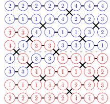
Figure 3. A wiring diagram of $a=0120312\in R(34\bar{2}\bar{1})$.

The wiring diagram of $a=a_{1}a_{2}\cdots a_{p}$ is the array $[p]\times[-n,n]$ in Cartesian coordinates. Each ordered pair in the array indexes a square cell, which may or may not contain a cross, denoted $\times$: specifically, the crosses are located at $(j,a_{j})$, and $(j,-a_{j})$ for all $1\leq j\leq p$ (thus if $a_{j}=0$, there will be just one cross in column $j$). The boundaries between cells $(u,v)$ and $(u,v+1)$, as well as the top and bottom edges of the diagram, contain a horizontal line denoted $\underline{\hskip 7.22743pt}$ unless there is a cross in the cell immediately above or below. The line segments connect with the crosses to form “wires” with labels $[-n]=\{-1,-2,\dots,-n\}$ and $[n]=\{1,2,\dots,n\}$ starting on the right hand edge of the diagram. So, specifically in the rightmost column, if $a_{p}>0$ then wires $a_{p}$ and $a_{p}+1$ cross in column $p$, and also wires $-a_{p}$ and $-a_{p}-1$ cross. If $a_{p}=0$, then wires $1$ and $-1$ cross in column $p$. For each $0\leq k<p$, define $w^{k}=s_{a_{p}}\dots s_{a_{k+1}}$, so that $w^{0}=w^{-1}$ and define $w^{p}$ to be the identity. The sequence of wire labels reading up along the left edge from bottom to top gives the long form of the signed permutation $w^{-1}$. More generally, the sequence of labels on the wires of the wiring diagram just to the right of column $k$ is the signed permutation $w^{k}$. Every wiring diagram should be considered as a subdiagram of the diagram with wires labeled by all of $\mathbb{Z}\setminus\{0\}$ where all constant trajectories above and below the diagram are suppressed in keeping with the notion that every signed permutation in $B_{n}$ can be thought of as an element of $B_{\infty}$. See Figure 3 for an illustration of these definitions.

The inversion set $\mbox{Inv}_{B}(w)$ of a signed permutation $w$ is

$$\mbox{Inv}_{B}(w)=\{(i,j)\in([-n]\cup[n])\times[n]:\ |i|\leq j\ \mbox{and}\ w(i)>w(j)\}.$$

We have defined the wiring diagrams so that the inversion $(i,j)$ corresponds with the crossing of wires $i$ and $j$ in any wiring diagram of a reduced word for $w$. Note, the wires $-j$ and $-i$ also cross in the same column in such a diagram. Thus, it is equivalent to refer to the inversion $(i,j)$ by $(-j,-i)$. If $a\in R(w)$, then the wiring diagram for $a$ is reduced and every crossing corresponds to an inversion for $w$.

For a word $a=a_{1}\dots a_{p}$ and $\delta\in\{-1,1\}$, we define a push $P^{\delta}_{i}$ at index $i$ to be the map that adds $\delta$ to $a_{i}$ while fixing the rest of the word provided $a_{i}$. If $a_{i}=0$, then regardless of $\delta$, the $i$th entry is set to $1$ in the resulting word e.g. $P^{-}_{1}(0)=P^{+}_{1}(0)=1$. We will write $P^{-}_{k}$ and $P^{+}_{k}$ for $\delta=-1$ and $\delta=1$ respectively. The effect pushes have on wiring diagrams can be observed in Figure 4.

If $a=a_{1}\dots a_{p}$ is a word that is not reduced, we say a defect is caused by $a_{i}$ and $a_{j}$ with $i\neq j$ if the removal of either leaves a reduced word. The following lemma can be deduced for signed permutations from the wiring diagrams, but it holds more generally for Coxeter groups.

Lemma 3.1.

[21, Lemma 21] For $W$ a Coxeter group and $w\in W$, let $a=a_{1}\dots\hat{a_{i}}\dots a_{p}\in R(w)$ such that $a_{1}\dots a_{p}$ is not reduced. Then there exists a unique $j\neq i$ such that $a_{1}\dots\hat{a_{j}}\dots a_{p}$ is reduced. Moreover, $a_{1}\dots\hat{a_{j}}\dots a_{p}\in R(w)$.

Definition 3.2 (Little Bump Algorithm).

Let $a=a_{1}\dots a_{p}$ be a reduced word of the signed permutation $w$ and $(i,j)\in\mbox{Inv}_{B}(w)$ such that $\ell(wt_{ij})=\ell(w)-1$. Fix $\delta\in\{-1,1\}$. We define the Little bump for $w$ at the inversion $(i,j)$ in the direction $\delta$, denoted $B^{\delta}_{(i,j)}$, as follows.

1. Identify the column $k$ and row $r$ containing the wire crossing $(i,j)$ with $i<j$. If $a_{k}=0$, set $b:=P^{1}_{k}(a)$ and $\delta:=-\delta$. If $a_{k}>0$, then either $w^{k}(a_{k})=i$ or $w^{k}(a_{k})=-j$. If $w^{k}(a_{k})=i$, set $b:=P^{\delta}_{k}(a)$. Otherwise $w^{k}(a_{k})=-j$, and we set $\delta:=-\delta$ and $b:=P^{\delta}_{k}(a)$. Next, set $r:=r+\delta$. Note that the order in which the variables are updated matters. Let $(x<y)$ be the new wires crossing in column $k$ and row $r$.

2. If $b$ is reduced, return $b$. Otherwise, by Lemma 3.1 there is a unique defect caused by $b_{k}$ and some $b_{l}$ with $l\neq k$. If $b_{l}>0$, then either $w^{l}(b_{l}+1)\in\{x,y\}$ or $w^{l}(b_{l}+1)\in\{-x,-y\}$. If $b_{l}=0$, then $x=-y$ and $w^{l}(1)\in\{-x,x\}$.

   • If $b_{l}>0$ and $w^{l}(b_{l}+1)\in\{x,y\}$, set $r:=r+\delta$, $k:=l$, and $b:=P^{\delta}_{k}(b)$. After updating the variables, let $(x<y)$ be the wires crossing in the diagram for $b$ in column $k$ and row $r$. Repeat Step 2.

   • Otherwise, $b_{l}=0$ or $w^{l}(b_{l}+1)\in\{-x,-y\}$. Set $\delta:=-\delta$, $r:=r+\delta$, $k:=l$ and $b:=P^{\delta}_{k}(b)$. Again, the order matters. After updating the variables, let $(x<y)$ be the wires crossing in column $k$ and row $r$. Repeat Step 2.

Figure 4 shows each step of a Little bump in terms of wiring diagrams. The corresponding effect on reduced words can be read off the diagrams by noting the row numbers of the wire crossings in the upper half plane including the $x$-axis.

Remark 3.3.

The Little bump algorithm is best thought of as acting on wiring diagrams. At every step, the pushes move the $(x,y)$-crossings consistently in the initial direction of $\delta$. In the first step, we move the $(i,j)$-crossing in the wiring diagram up if $\delta=+1$ and down if $\delta=-1$. If wires $i$ and $j$ cross in the upper half plane then the swap $a_{k}$ is replaced with $a_{k}+\delta$. However, if wires $i,j$ cross in the lower half plane then the swap $a_{k}$ is replaced with $a_{k}-\delta$ and the sign of $\delta$ is switched. If a new defect crossing is later found on the other side of the $x$-axis from the last crossing, then the sign of $\delta$ will switch again so that the crossing continues to move in the same direction. Thus, if the initial push moved $(i,j)$ down, each subsequent iteration will continue to move a crossing down, but the effect on the word from the corresponding push can vary.

Remark 3.4.

Observe that in each iteration of Step 2, the word $b$ has the property that its subword $b_{1}b_{2}\cdots\widehat{b_{k}}\cdots b_{p}$ is reduced.

When analyzing Little bumps and pushes, we will need to track where the next defect can occur. Given the wiring diagram for a word $b=b_{1}\cdots b_{p}$, not necessarily reduced, and a crossing $(x,y)$ in column $k$ in the diagram, define the (lower) boundary of $b$ for the crossing $(x,y)$, denoted $\partial^{k}_{(x,y)}(b)$, to be the union of the trajectory of $y$ from columns 0 to $k$ and the trajectory of $x$ from columns $k$ to $p$. Note using the notation of Step 2 above, if a defect is caused by $b_{k}$ in this iteration it will occur along $\partial^{k}_{(x,y)}(b)$. In Figure 4, the boundary of each crossing that will be pushed is dashed. A similar concept of an upper boundary could be defined if the initial step pushes the $(i,j)$ cross up.that

Lemma 3.5.

Let $a\in R(w)$ and $B^{\delta}_{(i,j)}$ be a Little bump for $w$ consisting of the sequence of pushes $P^{\delta_{1}}_{t_{1}},P^{\delta_{2}}_{t_{2}},\dots$ acting on $a$. Then, for all $k$ and $\delta\in\{-1,1\}$, the push $P^{\delta}_{k}$ appears at most once in this sequence. Hence, the Little bump algorithm terminates in at most $2\ell(w)$ pushes.

This proof is a slight extension of the proof of Lemma 5 in [25].

Proof.

Let $a=a_{1}a_{2}\dots a_{p}\in R(w)$ and $a_{k}$ denote the swap introducing the inversion $(i,j)$, with $i<j$. Since $B^{-}_{(i,j)}=B^{+}_{(-j,-i)}$, we need only demonstrate the result when the algorithm starts with a push that moves the $(i,j)$-crossing down.

In Step 1 of the Little bump algorithm, either $b=P^{\delta}_{k}(a)$ is reduced or there is some $l\neq k$ such that $b_{k}$ and $b_{l}$ cause a defect. Suppose the latter case holds. Then $b_{k}$ and $b_{l}$ swap the wire $i$ with some wire $h\neq i,j$. By considering the reverse of the word if necessary, we may assume $k<l$. The defect in column $l$ must occur on the boundary of $\partial^{k}_{(x,y)}(b)$. Observe that $\partial^{k}_{(i,j)}(a)$ and $\partial^{l}_{(i,h)}(b)$ coincide from 1 to $k$ and from $l$ to $p$. Moreover, between $k$ and $l$, the boundary $\partial^{l}_{(i,h)}(b)$ is strictly lower in the wiring diagram than $\partial^{k}_{(i,j)}(a)$. This can be seen in the first two diagrams shown in Figure 4. Observe that the trajectories of $-i$ and $-j$ will not interact with $\partial^{l}_{(i,h)}(b)$ unless $j=-i$. Therefore the boundary $\partial^{l}_{(i,h)}(b)$ is weakly below the boundary $\partial^{k}_{(i,j)}(a)$. Similar reasoning shows that on each iteration of Step 2 in the algorithm, the boundary always moves weakly down provided the initial push moves a crossing down.

Figure 4. The sequence of pushes corresponding to the Little bump $B^{-}_{(\overline{2},1)}$ as applied to $a=1021201\in R([1,\overline{3},\overline{2}])$. The boundary of each crossing about to be moved is dashed. Here, red is negative and blue is positive. The thin dashed line through the center row is row 0 and the row numbers increase going up.

$a=1021201$	$P^{-}_{3}(a)=1011201$
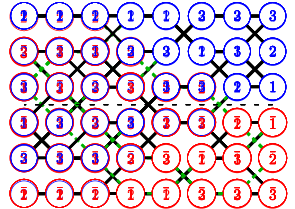
$P^{-}_{4}P^{-}_{3}(a)=1010201$	$P^{+}_{6}P^{-}_{4}P^{-}_{3}(a)=1010211$
$P^{+}_{7}P^{+}_{6}P^{-}_{4}P^{-}_{3}(a)=1010212$	$P^{-}_{1}P^{+}_{7}P^{+}_{6}P^{-}_{4}P^{-}_{3}(a)=0010212$

$P^{+}_{2}P^{-}_{1}P^{+}_{7}P^{+}_{6}P^{-}_{4}P^{-}_{3}(a)$	$P^{+}_{3}P^{+}_{2}P^{-}_{1}P^{+}_{7}P^{+}_{6}P^{-}_{4}P^{-}_{3}(a)$

$B^{-}_{(\overline{2},1)}(a)=P^{+}_{5}P^{+}_{3}P^{+}_{2}P^{-}_{1}P^{+}_{7}P^{+}_{6}P^{-}_{4}P^{-}_{3}(a)=0120312\in R([3,4,\overline{2},\overline{1}])$

Now we can verify that no push occurs twice in the Little bump algorithm. In particular, we claim that both $P_{k}^{-}$ and $P_{k}^{+}$ can occur, but they are never repeated. For example, $P^{-}_{5}$ and $P^{+}_{5}$ both occur in Figure 4. To do this, we need to examine the argument above more closely. Assume that Step 2 starts with a push $P_{k}^{\delta}$ moving a crossing into position $(k,r)$ in the wiring diagram of $b$. Assume this wiring diagram has a defect in columns $k$ and $l$ and $k<l$. Then the boundary before and after the push $P_{k}^{\delta}$ agree weakly to the left of column $k$. If successive pushes occur strictly to the right of column $k$, then none of these pushes will repeat $P_{k}^{\delta}$. Furthermore, the boundary to the left of column $k$ will be constant. The first time another iteration of Step 2 finds a defect weakly to the left of column $k$, we claim it must occur in a column strictly to the left of column $k$, thus the boundary moves strictly below $(k,r)$. The reason column $k$ cannot be part of the defect this time is that the boundary has negative slope just to the right of the crossing in row $r$ column $k$, but to create a defect with a string passing below $(k,r)$ the boundary must have positive slope where the two strings meet to the right of column $k$. Furthermore, if another push in column $k$ occurs later in the algorithm, it must be on the other side of the $x$-axis so it must be $P_{k}^{-\delta}$ since the boundary moves monotonically. Once the boundary has moved beyond both crossings in column $k$, neither crossing will be pushed again, so $P_{k}^{\delta}$ occurs at most once in the Little Bump algorithm. ∎

Lemma 3.6.

Let $w$ be a signed permutation, $a=a_{1}\dots a_{p}\in R(w)$, and $B^{\delta}_{(i,j)}$ be a Little bump for $w$. Then

$$peaks(a)=peaks(B^{\delta}_{(i,j)}(a)).$$

Proof.

Say $i\in peaks(a)$, so $a_{i-1}<a_{i}>a_{i+1}$. The statement holds unless a push applied to one of these entries during the algorithm leaves an equality in the resulting word $b$, say $b_{i-1}=b_{i}$. In this case, there is a defect caused by $b_{i-1}$ and $b_{i}$, so we push the other next. The direction of the new push for defects caused by adjacent entries will be the same unless $b_{i-1}=b_{i}=0$. This cannot occur since $a_{i}>a_{i-1}\geq 0$ and if $a_{i}=1$, then $a_{i-1}=0=a_{i+1}$. Hence, $a_{1}\dots\hat{a_{i}}\dots a_{p}$ would not be reduced, which is not possible by Remark 3.4. ∎

Theorem 3.7 (Restatement of Theorem 1.2, part 1).

Let $x\in B_{\infty}$, and let $a\in R(x)$. Say $j<k$.

1. If $B_{(j,k)}^{-}$ is a Little bump for $x$, then $B_{(j,k)}^{-}(a)\in R(xt_{jk}t_{ij})$ for some $i<j$.

2. If $B_{(j,k)}^{+}$ is a Little bump for $x$, then $B_{(j,k)}^{+}(a)\in R(xt_{jk}t_{kl})$ for some $k<l$.

Proof.

When applying $B^{-}_{(j,k)}$ on $a$, the initial push is some $P^{\delta_{1}}_{l_{1}}$ with $a_{1}\cdots\widehat{a_{l_{1}}}\cdots a_{p}\in R(v)$ for some $v\in B_{\infty}$. Let $b=P^{\delta_{1}}_{l_{1}}(a)$. Then, one can observe from the wiring diagrams that $s_{b_{1}}\cdots s_{b_{p}}=vt_{ji_{1}}$ for some $i_{1}\neq j,k$.

If $b$ is reduced, the bump is done. Otherwise, by the Little bump algorithm, there is some unique defect between $b_{l_{1}}$ and $b_{l_{2}}$ so we push next in column $l_{2}$. We know $b_{1}\cdots\widehat{b_{l_{2}}}\cdots b_{p}\in R(v)$ by construction and Remark 3.4. So when the next push occurs in column $l_{2}$ the new crossing will be between $j$ and another string $i_{2}$. Continuing the algorithm, we see recursively that $B^{-}_{(j,k)}(a)\in R(vt_{ji})$ for some $i\neq j,k$.

Assume for the sake of contradiction that $i>j$, and say the $(i,j)$-crossing in the wiring diagram of $c=B^{-}_{(j,k)}(a)$ occurs in column $l$. By removing the $l^{th}$ swap from $c$ we get a wiring diagram for $v$ that does not have $(j,i)$ as an inversion. Thus, the $i$-wire must stay entirely above the $j$-wire. Hence, the $i$ wire is above the boundary of the last push. Thus, it cannot be a part of the last push since the boundary moves monotonically according to the proof of Lemma 3.5. We can then conclude that $c\in R(vt_{ij})$ for some $i<j$.

A similar proof holds for the second statement. ∎

We recall the notation of transition equations from Section 1. If $w$ is not increasing, let $r$ be the largest value such that $w_{r}>w_{r+1}$. Define $s$ so that $(r<s)$ is the lexicographically largest pair of positive integers such that $w_{r}>w_{s}$. Set $v=wt_{rs}$. Let $T(w)$ be the set of all signed permutations $w^{\prime}=vt_{ir}$ for $i<r$, $i\neq 0$ such that $\ell(w^{\prime})=\ell(w)$.

Next, we show that the canonical Little bump $B_{(r,s)}^{-}$ for $w$ respects the transition equations in Theorem 2.15. This is best done by describing the domain and range of Little bumps in greater generality. For $v\in B_{\infty}$ and $j\in\mathbb{Z}-\{0\}$, we define

$$D(v,j) =\{vt_{ij}:\ i<j,\ i\neq 0\ \text{and}\ \ell(vt_{ij})=\ell(v)+1\}$$

$$U(v,j) =\{vt_{jk}:\ j<k,\ k\neq 0\ \text{and}\ \ell(vt_{jk})=\ell(v)+1\}.$$

Observe that we have $D(v,-j)=U(v,j)$. We now prove the analog of [25, Theorem 3], from which we can deduce Theorem 1.1.

Lemma 3.8.

Let $v\in B_{\infty}$ and $j\neq 0$. Then

$$\sum_{x\in U(v,j)}|R(x)|=\sum_{y\in D(v,j)}|R(y)|.$$

Proof.

We will prove the equality bijectively by using a collection of Little bumps. Define a map $M_{v,j}$ on $\cup_{x\in U(v,j)}R(x)$ as follows. Say $a=a_{1}\dots a_{p}\in R(x)$ for some $x\in U(v,j)$. Then $x=vt_{jk}$ for some unique $k>j$. Furthermore, $B^{-}_{(j,k)}$ is a Little bump for $x$. By Theorem 3.7, we know that $B^{-}_{(j,k)}(a)\in R(vt_{ij})$ for some $i<j$ and $\ell(vt_{ij})=\ell(vt_{jk})$. Thus, $vt_{ij}\in D(v,j)$. Set $M_{v,j}(a):=B^{-}_{(j,k)}(a)$ for all $a\in R(x)$. In this way, we construct a map

$$M_{v,j}:\cup_{x\in U(v,j)}R(x)\longrightarrow\cup_{y\in D(y,j)}R(y).$$

Since the Little bump algorithm is reversible with $B^{+}_{(i,j)}(c)=a$ in the notation above, we know $M_{v,j}$ is injective.

The bijective proof is completed by observing that $D(v,j)=U(v,-j)$, $U(v,j)=D(v,-j)$, and that $B^{-}_{(-j,-i)}=B^{+}_{(i,j)}$ is a Little bump for $vt_{ij}\in D(v,j)$ whose image, by the above argument, is a reduced word of some $x\in U(v,j)$. ∎

Corollary 3.9 (Restatement of Theorem 1.1).

Let $a\in R(w)$ and $B^{-}_{(r,s)}$ be the canonical Little bump for $w$. Recall that $(r,s)$ is the lexicographically last inversion in $w$. Then $B^{-}_{(r,s)}(a)$ is a reduced word for $w^{\prime}$ where

$$w^{\prime}\in T(w)=\{wt_{rs}t_{lr}\ \mid\ l<r\ \mbox{and}\ \ell(w)=\ell(wt_{rs}t_{rl})\}.$$

Proof.

Observe $U(wt_{rs},r)=\{w\}$ and

$$D(wt_{rs},r)=\{wt_{rs}t_{lr}\ \mid\ l<r,\ l\neq 0,\ \mbox{and}\ \ell(w)=\ell(wt_{rs}t_{rl})\}=T(w).$$

The result now follows from Lemma 3.8 with $v=wt_{rs}$ since $\ell(wt_{rs})=\ell(w)-1$ by choice of $(r,s)$. ∎

4. Kraśkiewicz insertion and the signed Little Bijection

In this section, we show that Coxeter-Knuth moves act on $Q^{\prime}(a)$ by shifted dual equivalence, as defined in [15]. We then prove the remainder of Theorem 1.2 by applying properties of shifted dual equivalence and showing that Little bumps and Coxeter-Knuth moves commute on reduced words of signed permutations.

For a permutation $\pi\in S_{n}$, let $\pi|_{I}$ be the subword consisting of values in the interval $I$. Let $\mathrm{fl}(\pi|_{I})\in S_{|I|}$ be the permutation with the same relative order as $\pi|_{I}$. Here $\mathrm{fl}$ is the flattening operator. Similarly, for $Q$ a standard shifted tableau $Q|_{I}$ denotes the shifted skew tableau obtained by restricting the tableau to the cells with values in the interval $I$.

Definition 4.1.

[15] Given a permutation $\pi\in S_{n}$, define the elementary shifted dual equivalence $h_{i}$ for all $1\leq i\leq n-3$ as follows. If $n\leq 3$, then $h_{1}(\pi)=\pi$. If $n=4$, then $h_{1}(\pi)$ acts by swapping $x$ and $y$ in the cases below,

(4.1) $$1x2y\quad x12y\quad 1x4y\quad x14y\quad 4x1y\quad x41y\quad 4x3y\quad x43y,$$

and $h_{1}(\pi)=\pi$ otherwise. If $n>4$, then $h_{i}$ is the involution that fixes values not in $I=\{i,i+1,i+2,i+3\}$ and permutes the values in $I$ via $\mathrm{fl}(h_{i}(\pi)|_{I})=h_{1}(\mathrm{fl}(\pi|_{I}))$.

As an example, $h_{1}(24531)=14532$, $h_{2}(25134)=24135$, and $h_{3}(314526)=314526$.

Recall from Definition 2.9 that a type B Coxeter-Knuth move starting at position $i$ is denoted by $\beta_{i}$. One can verify that this definition is equivalent to defining $h_{i}$ as

$$h_{i}(\pi)=(\beta_{i}(\pi^{-1}))^{-1}.$$

Given a standard shifted tableau $T$, we define $h_{i}(T)$ as the result of letting $h_{i}$ act on the row reading word of $T$. Observe $h_{i}(T)$ is also a standard shifted tableau. We can define an equivalence relation on standard shifted tableaux by saying $T$ and $h_{i}(T)$ are shifted dual equivalent for all $i$.

Theorem 4.2.

[15, Prop. 2.4] Two standard shifted tableaux are shifted dual equivalent if and only if they have the same shape.

Recall the notion of jeu de taquin is an algorithm for sliding one cell at a time in a standard tableau on a skew shape in such a way that the result is still a standard tableau [28]. The analogous notion for shifted tableaux was introduced independently in [29] and [34].

Lemma 4.3.

[15, Lemma 2.3] Given two standard shifted tableaux $T$ and $U$ with $T=h_{i}(U)$, let $T^{\prime}$ and $U^{\prime}$ be the result of applying any fixed sequence of jeu de taquin slides to $T$ and $U$, respectively. Then $T^{\prime}=h_{i}(U^{\prime})$.

Definition 4.4.

Given a standard shifted tableau $Q^{\prime}$, define $\Delta(Q^{\prime})$ as the result of removing the cell containing 1, performing jeu de taquin into this now empty cell, and subtracting 1 from the value of each of the cells in the resulting tableau.

Lemma 4.5.

[22, Theorem 3.24] Let $w$ be a signed permutation and $a=a_{1}\cdots a_{p}\in R(w)$. Then under Kraśkiewicz insertion

(4.2) $$Q^{\prime}(a_{2}\cdots a_{p})=\Delta(Q^{\prime}(a_{1}\cdots a_{p})).$$

Lemma 4.6.

Let $w$ be a signed permutation, and let $a=a_{1}\dots a_{p}\in R(w)$. Then $Q^{\prime}(\beta_{i}(a))=h_{i}(Q^{\prime}(a))$ for all integers $1\leq i\leq p-3$.

Proof.

Recall that $\beta_{i}$ acts trivially on $a$ if and only if both $i+1,i+2\notin peaks(a)$. Similarly, $h_{i}$ acts trivially on $Q^{\prime}(a)$ if and only if both $i+1,i+2\notin peaks(Q^{\prime}(a))$. By Theorem 2.8, we then see $\beta_{i}$ acts trivially if and only if $h_{i}$ acts trivially. Thus, the lemma holds if both $h_{i}$ and $\beta_{i}$ act trivially so we will assume that this is not the case.

Since type B Coxeter-Knuth moves preserve Kraśkiewicz insertion tableaux, we see $Q^{\prime}(a)|_{[1,i-1]}=Q^{\prime}(\beta_{i}(a))|_{[1,i-1]}$, $Q^{\prime}(a)|_{[i+4,p]}=Q^{\prime}(\beta_{i}(a))|_{[i+4,p]}$ and that the shape of $Q^{\prime}(a)|_{[i,i+3]}$ and $Q^{\prime}(\beta_{i}(a))|_{[i,i+3]}$ are the same. In particular, $Q^{\prime}(a)$ differs from $Q^{\prime}(\beta_{i}(a))$ by some rearrangement of the values in $[i,i+3]$. We need to show that this rearrangement is the elementary shifted dual equivalence $h_{i}$. The following proof of this fact is presented as a commuting diagram in Figure 5.

By omitting any extra values at the end of $a$, we may assume that $p=i+3$. Now consider the tableaux $T$ and $U$ obtained by adding $i-1$ to each entry in $\Delta^{i-1}(Q^{\prime}(a))$ and $\Delta^{i-1}(Q^{\prime}(\beta_{i}(a))$. Because $Q^{\prime}(a)|_{[1,i-1]}=Q^{\prime}(\beta_{i}(a))|_{[1,i-1]}$, it follows from the definition of $\Delta$ that there is some fixed set of jeu de taquin slides that relates both $Q^{\prime}(a)|_{[i,i+3]}$ to $T$ and $Q^{\prime}(\beta_{i}(a))|_{[i,i+3]}$ to $U$. Applying Lemma 4.3, we need only show that $T=h_{i}(U)$ to complete the proof.

By Lemma 4.5, we see

$$\Delta^{i-1}(Q^{\prime}(a))=Q^{\prime}(a_{i}a_{i+1}a_{i+2}a_{i+3})$$

and

$$\Delta^{i-1}(Q^{\prime}(\beta_{i}(a)))=Q^{\prime}(\beta_{1}(a_{i}a_{i+1}a_{i+2}a_{i+3})).$$

Since $Q^{\prime}(\beta_{1}(a_{i}a_{i+1}a_{i+2}a_{i+3}))$ and $Q^{\prime}(a_{i}a_{i+1}a_{i+2}a_{i+3})$ are distinct by assumption and are necessarily standard tableaux of the same shifted shape with four cells, the shape must be $(3,1)$. Furthermore, there are only two standard tableaux of shifted shape $(3,1)$, so the two tableaux must be related by $Q^{\prime}(\beta_{1}(a_{1}a_{2}a_{3}a_{4}))=h_{1}(Q^{\prime}(a_{1}a_{2}a_{3}a_{4}))$. Adding $i-1$ to each entry of the two tableaux in this equation changes $h_{1}$ to $h_{i}$ and yields the desired result, $T=h_{i}(U)$. ∎

Figure 5. The commuting relationships in the proof of Proposition 4.6 on top and a generic example on bottom.

Next, we show that Coxeter-Knuth moves commute with Little bumps.

Lemma 4.7.

Let $a=a_{1}\dots a_{p}$ be a reduced word of the signed permutation $w$, $\beta_{k}$ a Coxeter-Knuth move for $a$ and $B^{\delta}_{(i,j)}$ a Little bump for $w$. Then

$$B^{\delta}_{(i,j)}(\beta_{k}(a))=\beta_{k}(B^{\delta}_{(i,j)}(a)).$$

Proof.

First, observe that a Little bump and the Coxeter-Knuth move $\beta_{k}$ will only interact if one of the pushes in the bump is applied to an entry in the window $[k,k+3]$. The inversions introduced by $a_{i}$ and $\beta_{k}(a)_{i}$ are the same when $i\not\in[k,k+3]$. Therefore, since $a$ and $\beta_{k}(a)$ are reduced words of the same permutation, we see the inversions introduced by $a_{k}a_{k+1}a_{k+2}a_{k+3}$ in $a$ and $\beta_{k}(a_{k}a_{k+1}a_{k+2}a_{k+3})$ in $\beta_{k}(a)$ are the same as well. Therefore if a crossing with index in $[k,k+3]$ is pushed when a Little bump $B^{\delta}_{(i,j)}$ is applied to $a$, such a crossing will also be pushed when $B^{\delta}_{(i,j)}$ is applied to $\beta_{k}(a)$, though not necessarily the same position. Our argument relies on showing commutation can be reduced to a local check of how $\beta_{k}$ interacts with $B^{\delta}_{(i,j)}$. In particular, the result will follow from establishing two properties:

1. $B^{\delta}_{(i,j)}(a)$ and $B^{\delta}_{(i,j)}(\beta_{k}(a))$ also differ by a Coxeter-Knuth move at position $k$.

2. The final push to a swap acted on by the Coxeter-Knuth move has the same effect on $w$ for both $a$ and $\beta_{k}(a)$, hence would introduce the same defect should the bump continue.

When the entries acted on by a Coxeter-Knuth move differ by two or more, these properties are trivial to confirm. For entries that are closer, the features can be checked for each type of Coxeter-Knuth move either by hand or by computer program. There are as many as four checks for each type of Coxeter-Knuth move, depending on the initial inversion and whether $0$ appears in the word. These can be performed by verifying the result for all possible bumps on reduced words in $B_{5}$ of length 4. See Figure 6 for example. ∎

Figure 6. $B^{-}_{(1,2)}(1010)$ compared to $B^{-}_{(1,2)}(0101)$. The results differ by a Coxeter-Knuth move and the final pushes introduce the same transposition.

Notice that if we weakly order all shifted standard tableaux of shape $\lambda$ by their peak sets in lexicographical order, then the unique maximal element $U_{\lambda}$ is obtained by placing $1$ through $\lambda_{1}$ in the first row, $\lambda_{1}+1$ through $\lambda_{1}+\lambda_{2}$ in the second row, and so on. Further notice that $peaks(U_{\lambda})=\{\lambda_{1},\lambda_{1}+\lambda_{2},\lambda_{1}+\lambda_{2}+\lambda_{3},\ldots\}$.

Lemma 4.8.

Let $w$ be a signed permutation, $a\in R(w)$, $B^{\delta}_{(i,j)}$ be a Little bump for $w$ and $b=B^{\delta}_{(i,j)}(a)$. Then $Q^{\prime}(a)=Q^{\prime}(b)$.

Proof.

We first show that $Q^{\prime}(a)$ and $Q^{\prime}(b)$ have the same shape. By Lemma 2.8 and Lemma 3.6,

$$peaks(Q^{\prime}(a))=peaks(a)=peaks(b)=peaks(Q^{\prime}(b)).$$

Let $a^{\prime}$ and $b^{\prime}$ be the reduced words with maximal peak sets in the Coxeter-Knuth class of $a$ and $b$, respectively. Applying Lemma 4.7, we may assume that $a=a^{\prime}$. The shape of $Q^{\prime}(a^{\prime})=U_{\lambda}$ is determined by its peak set. Hence, the shape of $Q^{\prime}(b)$ must be at least as large as the shape of $Q^{\prime}(a)$ in dominance order. By assuming that $b=b^{\prime}$, we can conclude the converse. Hence, $Q^{\prime}(a)$ and $Q^{\prime}(b)$ have the same shape $\lambda$. Furthermore, $Q^{\prime}(a^{\prime})=U_{\lambda}=Q^{\prime}(b^{\prime})$.

We now proceed to showing that $Q^{\prime}(a)=Q^{\prime}(b)$. By Theorem 2.10, there exists a sequence of Coxeter-Knuth moves $\beta=\beta_{i_{1}}\circ\beta_{i_{2}}\circ\cdots\circ\beta_{i_{k}}$ such that $\beta(a^{\prime})=a$. From Lemma 4.6, we see

$$Q^{\prime}(a)=Q^{\prime}(\beta(a^{\prime}))=h_{i_{1}}\dots h_{i_{k}}(U_{\lambda}).$$

Applying Lemma 4.7, $\beta(b^{\prime})=b$, so

$$Q^{\prime}(b)=Q^{\prime}(\beta(b^{\prime}))=h_{i_{1}}\dots h_{i_{k}}(U_{\lambda}),$$

from which we conclude that $Q^{\prime}(a)=Q^{\prime}(b)=Q^{\prime}(B^{\delta}_{(i,j)}(a))$. ∎

As a consequence of Lemma 4.8, we prove an analog of Thomas Lam’s conjecture for signed permutations. Two reduced words $a$ and $b$ communicate if there exists a sequence of Little bumps $B^{\delta_{1}}_{1},B^{\delta_{2}}_{2},\dots,B^{\delta_{n}}_{n}$ such that $b=B^{\delta_{n}}_{n}(\dots B^{\delta_{1}}_{1}(a))$. Since Little bumps are invertible, this defines an equivalence relation.

Theorem 4.9 (Restatement of Theorem 1.2, part 2).

Let $a$ and $b$ be reduced words. Then $Q^{\prime}(a)=Q^{\prime}(b)$ if and only if they communicate via Little bumps.

Proof.

If $a$ and $b$ communicate, then we see $Q^{\prime}(a)=Q^{\prime}(b)$ by Lemma 4.8. Therefore we only need to prove the converse.

Let $Q=Q^{\prime}(a)=Q^{\prime}(b)$. We show that $a$ and $b$ both communicate with some reduced word $c$ uniquely determined by $Q$. Since communication is an equivalence relation, this will complete our proof. Recall from Theorem 2.15 that by repeated application of the transition equations, we may express any C-Stanley symmetric function as the sum of C-Stanley symmetric functions of increasing signed permutations. Since canonical Little bumps follow the transition equations by Corollary 3.9, repeated applications of canonical Little bumps will transform any reduced word $a$ into some reduced word $c$ of an increasing permutation $u$. Since $a$ and $c$ communicate, $Q^{\prime}(a)=Q^{\prime}(c)$. By Equation (2.3) and the fact that $u$ is increasing, $F_{u}(X)=Q_{\mu}(X)$ for some $\mu$ and the reduced expressions for $u$ are in bijection with the standard tableaux of shifted shape $\mu$ under Kraśkiewicz insertion. This implies that $c$ is uniquely determined by $Q^{\prime}(a)$, and hence for $Q^{\prime}(b)$ as well. Therefore, every reduced word $a$ with $Q^{\prime}(a)=Q$ communicates with the same word $c\in R(u)$. ∎

Corollary 4.10.

[Restatement of Theorem 1.2, part 3] Every communication class under signed Little bumps has a unique reduced word for an increasing signed permutation.

For permutations, Theorem 3.32 in [22] shows that Kraśkiewicz insertion coincides with Haiman’s shifted mixed insertion. From this, we can conclude the following.

Corollary 4.11.

Let $\{j_{1}<j_{2}<...<j_{p}\}$ be an increasing sequence of $p$ distinct non-negative integers. Every communication class containing words of length $p$ under signed Little bumps contains a reduced word that is a permutation of $\{j_{1},j_{2},...,j_{p}\}$.

This result can also be proved using Little bumps.

5. Axioms for shifted dual equivalence graphs

In this section, we build on the connection between shifted dual equivalence operators $h_{i}$ and type B Coxeter-Knuth moves $\beta_{i}$ as stated in Lemma 4.6. In particular, we define and classify the shifted dual equivalence graphs associated to these operators via two local properties. Along the way, we also demonstrate several important properties of these graphs. The approach is analogous to the axiomatization of dual equivalence graphs by Assaf [3], which was later refined by Roberts [27].

Definition 5.1.

Fix a strict partition $\lambda\vdash n$. By definition, $h_{i}$ acts as an involution on the standard shifted tableaux of shape $\lambda$, denoted $SST(\lambda)$. Given $\lambda$, define the standard shifted dual equivalence graph of degree $n$ for $\lambda$, denoted

$$\mathcal{SG}_{\lambda}=(V,\sigma,E_{1}\cup\ldots\cup E_{n-3})$$

as follows. The vertex set $V$ is $SST(\lambda)$, and the labeled edge sets $E_{i}$ for $1\leq i\leq n-3$ are given by the nontrivial orbits of $h_{i}$ on $SST(\lambda)$. To define the signature $\sigma$, recall from Section 2 that every tableau $T\in SST(\lambda)$ has a peak set, denoted $peaks(T)$. We encode a peak set by a sequence of pluses and minuses denoted $\sigma(T)\in\{+,-\}^{n}$, where $\sigma_{i}(T)=+$ if and only if $i$ is a peak in $T$. We refer to $\sigma(T)$ as the signature of $T$. Note that peaks never occur in positions 1 or $n$ and that they never occur consecutively. Conversely, any subset of $[n]$ that satisfies these properties is the peak set of some tableau, hence we will call it an admissible peak set.

aligntableaux=center, smalltableaux

$$\begin{array}[]{c}\vbox{\vbox{ \lx@xy@svg{\hbox{\raise 0.0pt\hbox{\kern 16.6743pt\hbox{\ignorespaces\ignorespaces\ignorespaces\hbox{\vtop{\kern 0.0pt\offinterlineskip\halign{\entry@#!@&&\entry@@#!@\cr\crcr}}}\ignorespaces{\hbox{\kern-16.6743pt\raise 0.0pt\hbox{\hbox{\kern 0.0pt\raise 0.0pt\hbox{\hbox{\kern 3.0pt\raise 0.0pt\hbox{$\textstyle{{\ytableaushort{123456}\atop----}}$}}}}}}}\ignorespaces}}}}\ignorespaces}}\\ \vbox{\vbox{ \lx@xy@svg{\hbox{\raise 0.0pt\hbox{\kern 21.65413pt\hbox{\ignorespaces\ignorespaces\ignorespaces\hbox{\vtop{\kern 0.0pt\offinterlineskip\halign{\entry@#!@&&\entry@@#!@\cr&&&\crcr}}}\ignorespaces{\hbox{\kern-21.65413pt\raise 0.0pt\hbox{\hbox{\kern 0.0pt\raise 0.0pt\hbox{\hbox{\kern 3.0pt\raise 0.0pt\hbox{$\textstyle{{\ytableaushort{\none 3,12456}\atop+---}\ignorespaces\ignorespaces\ignorespaces\ignorespaces}$}}}}}}}\ignorespaces\ignorespaces\ignorespaces\ignorespaces{}{\hbox{\lx@xy@droprule}}\ignorespaces\ignorespaces\ignorespaces{\hbox{\kern 28.90413pt\raise 5.25555pt\hbox{{}\hbox{\kern 0.0pt\raise 0.0pt\hbox{\hbox{\kern 3.0pt\hbox{\hbox{\kern 0.0pt\raise-2.25555pt\hbox{$\scriptstyle{1}$}}}\kern 3.0pt}}}}}}\ignorespaces{}{\hbox{\lx@xy@droprule}}{\hbox{\lx@xy@droprule}}{\hbox{\kern 45.65413pt\raise 0.0pt\hbox{\hbox{\kern 0.0pt\raise 0.0pt\hbox{\hbox{\kern 3.0pt\raise 0.0pt\hbox{$\textstyle{{\ytableaushort{\none 4,12356}\atop-+--}\ignorespaces\ignorespaces\ignorespaces\ignorespaces}$}}}}}}}\ignorespaces\ignorespaces\ignorespaces\ignorespaces{}{\hbox{\lx@xy@droprule}}\ignorespaces\ignorespaces\ignorespaces{\hbox{\kern 96.21239pt\raise 5.25555pt\hbox{{}\hbox{\kern 0.0pt\raise 0.0pt\hbox{\hbox{\kern 3.0pt\hbox{\hbox{\kern 0.0pt\raise-2.25555pt\hbox{$\scriptstyle{2}$}}}\kern 3.0pt}}}}}}\ignorespaces{}{\hbox{\lx@xy@droprule}}{\hbox{\lx@xy@droprule}}{\hbox{\kern 112.96239pt\raise 0.0pt\hbox{\hbox{\kern 0.0pt\raise 0.0pt\hbox{\hbox{\kern 3.0pt\raise 0.0pt\hbox{$\textstyle{{\ytableaushort{\none 5,12346}\atop--+-}\ignorespaces\ignorespaces\ignorespaces\ignorespaces}$}}}}}}}\ignorespaces\ignorespaces\ignorespaces\ignorespaces{}{\hbox{\lx@xy@droprule}}\ignorespaces\ignorespaces\ignorespaces{\hbox{\kern 163.52065pt\raise 5.25555pt\hbox{{}\hbox{\kern 0.0pt\raise 0.0pt\hbox{\hbox{\kern 3.0pt\hbox{\hbox{\kern 0.0pt\raise-2.25555pt\hbox{$\scriptstyle{3}$}}}\kern 3.0pt}}}}}}\ignorespaces{}{\hbox{\lx@xy@droprule}}{\hbox{\lx@xy@droprule}}{\hbox{\kern 180.27065pt\raise 0.0pt\hbox{\hbox{\kern 0.0pt\raise 0.0pt\hbox{\hbox{\kern 3.0pt\raise 0.0pt\hbox{$\textstyle{{\ytableaushort{\none 6,12345}\atop---+}}$}}}}}}}\ignorespaces}}}}\ignorespaces}}\\ \vbox{\vbox{ \lx@xy@svg{\hbox{\raise 0.0pt\hbox{\kern 21.65413pt\hbox{\ignorespaces\ignorespaces\ignorespaces\hbox{\vtop{\kern 0.0pt\offinterlineskip\halign{\entry@#!@&&\entry@@#!@\cr&&&&\crcr}}}\ignorespaces{\hbox{\kern-21.65413pt\raise 0.0pt\hbox{\hbox{\kern 0.0pt\raise 0.0pt\hbox{\hbox{\kern 3.0pt\raise 0.0pt\hbox{$\textstyle{{\ytableaushort{\none 45,1236}\atop-+--}\ignorespaces\ignorespaces\ignorespaces\ignorespaces}$}}}}}}}\ignorespaces\ignorespaces\ignorespaces\ignorespaces{}{\hbox{\hbox{\kern 0.0pt\raise 1.0pt\hbox{\lx@xy@droprule}}\hbox{\kern 0.0pt\raise-1.0pt\hbox{\lx@xy@droprule}}}}\ignorespaces\ignorespaces\ignorespaces{\hbox{\kern 28.90413pt\raise 5.25555pt\hbox{{}\hbox{\kern 0.0pt\raise 0.0pt\hbox{\hbox{\kern 3.0pt\hbox{\hbox{\kern 0.0pt\raise-2.25555pt\hbox{$\scriptstyle{1}$}}}\kern 3.0pt}}}}}}\ignorespaces\ignorespaces\ignorespaces{\hbox{\kern 28.90413pt\raise-5.25555pt\hbox{{}\hbox{\kern 0.0pt\raise 0.0pt\hbox{\hbox{\kern 3.0pt\hbox{\hbox{\kern 0.0pt\raise-2.25555pt\hbox{$\scriptstyle{2}$}}}\kern 3.0pt}}}}}}\ignorespaces{}{\hbox{\hbox{\kern 0.0pt\raise 1.0pt\hbox{\lx@xy@droprule}}\hbox{\kern 0.0pt\raise-1.0pt\hbox{\lx@xy@droprule}}}}{\hbox{\hbox{\kern 0.0pt\raise 1.0pt\hbox{\lx@xy@droprule}}\hbox{\kern 0.0pt\raise-1.0pt\hbox{\lx@xy@droprule}}}}{\hbox{\kern 45.65413pt\raise 0.0pt\hbox{\hbox{\kern 0.0pt\raise 0.0pt\hbox{\hbox{\kern 3.0pt\raise 0.0pt\hbox{$\textstyle{{\ytableaushort{\none 35,1246}\atop+-+-}\ignorespaces\ignorespaces\ignorespaces\ignorespaces}$}}}}}}}\ignorespaces\ignorespaces\ignorespaces\ignorespaces{}{\hbox{\lx@xy@droprule}}\ignorespaces\ignorespaces\ignorespaces{\hbox{\kern 96.21239pt\raise 5.25555pt\hbox{{}\hbox{\kern 0.0pt\raise 0.0pt\hbox{\hbox{\kern 3.0pt\hbox{\hbox{\kern 0.0pt\raise-2.25555pt\hbox{$\scriptstyle{3}$}}}\kern 3.0pt}}}}}}\ignorespaces{}{\hbox{\lx@xy@droprule}}{\hbox{\lx@xy@droprule}}{\hbox{\kern 112.96239pt\raise 0.0pt\hbox{\hbox{\kern 0.0pt\raise 0.0pt\hbox{\hbox{\kern 3.0pt\raise 0.0pt\hbox{$\textstyle{{\ytableaushort{\none 36,1245}\atop+--+}\ignorespaces\ignorespaces\ignorespaces\ignorespaces}$}}}}}}}\ignorespaces\ignorespaces\ignorespaces\ignorespaces{}{\hbox{\lx@xy@droprule}}\ignorespaces\ignorespaces\ignorespaces{\hbox{\kern 163.52065pt\raise 5.25555pt\hbox{{}\hbox{\kern 0.0pt\raise 0.0pt\hbox{\hbox{\kern 3.0pt\hbox{\hbox{\kern 0.0pt\raise-2.25555pt\hbox{$\scriptstyle{1}$}}}\kern 3.0pt}}}}}}\ignorespaces{}{\hbox{\lx@xy@droprule}}{\hbox{\lx@xy@droprule}}{\hbox{\kern 180.27065pt\raise 0.0pt\hbox{\hbox{\kern 0.0pt\raise 0.0pt\hbox{\hbox{\kern 3.0pt\raise 0.0pt\hbox{$\textstyle{{\ytableaushort{\none 46,1235}\atop-+-+}\ignorespaces\ignorespaces\ignorespaces\ignorespaces}$}}}}}}}\ignorespaces\ignorespaces\ignorespaces\ignorespaces{}{\hbox{\hbox{\kern 0.0pt\raise 1.0pt\hbox{\lx@xy@droprule}}\hbox{\kern 0.0pt\raise-1.0pt\hbox{\lx@xy@droprule}}}}\ignorespaces\ignorespaces\ignorespaces{\hbox{\kern 230.8289pt\raise 5.25555pt\hbox{{}\hbox{\kern 0.0pt\raise 0.0pt\hbox{\hbox{\kern 3.0pt\hbox{\hbox{\kern 0.0pt\raise-2.25555pt\hbox{$\scriptstyle{2}$}}}\kern 3.0pt}}}}}}\ignorespaces\ignorespaces\ignorespaces{\hbox{\kern 230.8289pt\raise-5.25555pt\hbox{{}\hbox{\kern 0.0pt\raise 0.0pt\hbox{\hbox{\kern 3.0pt\hbox{\hbox{\kern 0.0pt\raise-2.25555pt\hbox{$\scriptstyle{3}$}}}\kern 3.0pt}}}}}}\ignorespaces{}{\hbox{\hbox{\kern 0.0pt\raise 1.0pt\hbox{\lx@xy@droprule}}\hbox{\kern 0.0pt\raise-1.0pt\hbox{\lx@xy@droprule}}}}{\hbox{\hbox{\kern 0.0pt\raise 1.0pt\hbox{\lx@xy@droprule}}\hbox{\kern 0.0pt\raise-1.0pt\hbox{\lx@xy@droprule}}}}{\hbox{\kern 247.5789pt\raise 0.0pt\hbox{\hbox{\kern 0.0pt\raise 0.0pt\hbox{\hbox{\kern 3.0pt\raise 0.0pt\hbox{$\textstyle{{\ytableaushort{\none 56,1234}\atop--+-}}$}}}}}}}\ignorespaces}}}}\ignorespaces}}\\ \vbox{\vbox{ \lx@xy@svg{\hbox{\raise 0.0pt\hbox{\kern 30.36382pt\hbox{\ignorespaces\ignorespaces\ignorespaces\hbox{\vtop{\kern 0.0pt\offinterlineskip\halign{\entry@#!@&&\entry@@#!@\cr&\crcr}}}\ignorespaces{\hbox{\kern-30.36382pt\raise 0.0pt\hbox{\hbox{\kern 0.0pt\raise 0.0pt\hbox{\hbox{\kern 3.0pt\raise 0.0pt\hbox{$\textstyle{{\ytableaushort{\none\none 6,\none 35,124}\atop+-+-}\;\ignorespaces\ignorespaces\ignorespaces\ignorespaces}$}}}}}}}\ignorespaces\ignorespaces\ignorespaces\ignorespaces{}{\hbox{\hbox{\kern 0.0pt\raise 2.0pt\hbox{\lx@xy@droprule}}\hbox{\kern 0.0pt\raise-2.0pt\hbox{\lx@xy@droprule}}\hbox{\lx@xy@droprule}}}\ignorespaces\ignorespaces\ignorespaces{\hbox{\kern 31.47495pt\raise 5.93611pt\hbox{{}\hbox{\kern 0.0pt\raise 0.0pt\hbox{\hbox{\kern 3.0pt\hbox{\hbox{\kern 0.0pt\raise-1.57501pt\hbox{$\scriptstyle{1,2,3}$}}}\kern 3.0pt}}}}}}\ignorespaces{}{\hbox{\hbox{\kern 0.0pt\raise 2.0pt\hbox{\lx@xy@droprule}}\hbox{\kern 0.0pt\raise-2.0pt\hbox{\lx@xy@droprule}}\hbox{\lx@xy@droprule}}}{\hbox{\hbox{\kern 0.0pt\raise 2.0pt\hbox{\lx@xy@droprule}}\hbox{\kern 0.0pt\raise-2.0pt\hbox{\lx@xy@droprule}}\hbox{\lx@xy@droprule}}}{\hbox{\kern 54.36382pt\raise 0.0pt\hbox{\hbox{\kern 0.0pt\raise 0.0pt\hbox{\hbox{\kern 3.0pt\raise 0.0pt\hbox{$\textstyle{{\ytableaushort{\none\none 6,\none 45,123}\atop-+-+}}$}}}}}}}\ignorespaces}}}}\ignorespaces} }\end{array}$$

Figure 7. The standard shifted dual equivalence graphs of degree 6 omitting $\sigma_{1}$ and $\sigma_{6}$.

In Figure 7, all of the standard shifted dual equivalence graphs of degree 6 are drawn and labeled by their signatures omitting $\sigma_{1}$ and $\sigma_{6}$ since $1$ and $6$ can never be in an admissible peak set. Already from this figure we can see that standard shifted dual equivalence graphs are not always dual equivalence graphs because they can have two vertices connected by 3 edges labeled $i,i+1,i+2$. Also, observe that if vertices $v$ and $w$ are contained in an $i$-edge, then $\sigma_{[i+1,i+2]}(v)=-\sigma_{[i+1,i+2]}(w)$. Furthermore, notice that the label $i$ of the edge and whether or not it is a double or triple edge can be determined entirely from the peak sets. This fact will be used often in the proofs that follow. From this figure, we also can determine all of the possible standard shifted dual equivalence graphs for $n=1,2,3,4,5$ by fixing the values higher than $n$.

The standard shifted dual equivalence graphs have several nice properties on par with the dual equivalence graphs or equivalently Coxeter-Knuth graphs of type $A$. By Theorem 4.2, each $\mathcal{SG}_{\lambda}$ is connected. Observe that by Definition 2.12, a Schur $Q$-function $Q_{\lambda}$ is the generating function for the sum of peak quasisymmetric functions associated to the labels on the vertices of $\mathcal{SG}_{\lambda}$. Recall from Section 4 that the lexicographically largest peak set for all standard shifted tableaux of a fixed shape $\lambda$ is given by the unique tableau $U_{\lambda}$. Thus, the shape $\lambda$ can be recovered from the multiset of signatures on the vertices.

Each standard shifted dual equivalence graph is an example of the following more general type of graph.

Definition 5.2.

Let $C$ and $S$ be two finite ordered lists. An $S$-signed, $C$-colored graph consists of the following data:

1. a finite vertex set $V$,

2. a signature function $\sigma:V\rightarrow\{+,-\}^{|S|}$ associating a subset of $S$ to each vertex,

3. a collection $E_{i}$ of unordered pairs of distinct vertices in $V$ for each $i\in C$.

A signed colored graph is denoted $\mathcal{G}=(V,\sigma,E)$ where $E=\cup_{i\in C}E_{i}$. We say that $\mathcal{G}$ has shifted degree n if $C=[n-3]$, $S=[n]$ and $\sigma(v)$ is an admissible peak set for an integer sequence of length $n$ for all $v\in V$. The signature $\sigma(v)$ is encoded by a sequence in $\{+,-\}^{n}$ where $\sigma_{i}(v)=+$ if and only if $i\in\sigma(v)$. We use the notation $\sigma_{[i,j]}(v)$ to mean the subset $\sigma(v)\cap[i,j]$ which can be encoded by $+$’s and $-$’s as well.

Definition 5.3.

Given two $S$-signed $C$-colored graphs $\mathcal{G}=(V,\sigma,E)$ and $\mathcal{G}^{\prime}=(V^{\prime},\sigma^{\prime},E^{\prime})$, a morphism of signed colored graphs $\phi\colon G\to G^{\prime}$ is a map from $V$ to $V^{\prime}$ that preserves the signature function and induces a map from $E_{i}$ into $E^{\prime}_{i}$ for all $i\in C$. An isomorphism is a morphism that is a bijection on the vertices such that the inverse is also a morphism.

Definition 5.4.

A signed colored graph $\mathcal{G}$ is a shifted dual equivalence graph (SDEG) if it is isomorphic to a disjoint union of standard shifted dual equivalence graphs.

The next lemma allows us to classify the isomorphism type of any connected SDEG by a unique standard shifted dual equivalence graph.

Lemma 5.5.

Let $\mathcal{SG}_{\lambda}$ and $\mathcal{SG}_{\mu}$ be any two standard shifted dual equivalence graphs. If $\phi\colon\mathcal{SG}_{\lambda}\to\mathcal{SG}_{\mu}$ is an isomorphism, then $\lambda=\mu$ and $\phi$ is the identity map.

Proof.

Suppose that $\phi:\mathcal{SG}_{\lambda}\to\mathcal{SG}_{\mu}$ is an isomorphism. Then the vertices of $\mathcal{SG}_{\lambda}$ and $\mathcal{SG}_{\mu}$ must have the same multisets of associated peak sets. By looking at the unique lexicographically maximal peak set in both, it follows that $U_{\lambda}=U_{\mu}$. In particular, $\lambda=\mu$. Thus, $\phi$ is an automorphism that sends $U_{\lambda}$ to itself. Since $h_{i}$ defines the $i$-edges in both $\mathcal{SG}_{\lambda}$ and $\mathcal{SG}_{\mu}$ and both graphs are connected, we see that $\phi$ acts as the identity map. ∎

The connection between shifted dual equivalence graphs and the type B Coxeter-Knuth graphs stated in Theorem 1.3 is now readily apparent. Recall, Theorem 1.3 states that every type B Coxeter-Knuth graph $CK_{B}(w)$ with signature function given by peak sets is a shifted dual equivalence graph, where the isomorphism is given by the Kraśkiewicz $Q^{\prime}$ function. It further states that every shifted dual equivalence graph is also isomorphic to some $CK_{B}(w)$. We give the proof of this theorem now.

Proof of Theorem 1.3.

We show that the map $Q^{\prime}$ sending vertices in $CK_{B}(w)$ to their recording tableaux is the desired isomorphism. This follows immediately from the definition of the Kraśkiewicz insertion algorithm, Lemma 2.8 and Lemma 4.6.

To see the converse statement, observe that $\mathcal{SG}_{\mu}$ is isomorphic to the Coxeter-Knuth graph $CK_{B}(w)$ for the increasing signed permutation $w=w(\mu)$ as defined just before Equation 2.3. ∎

Definition 5.6.

Given a signed colored graph $\mathcal{G}=(V,\sigma,E)$ of shifted degree $n$ and an interval of nonnegative integers $I=[a,b]\subset[n]$, let

$$\mathcal{G}^{I}=\left(V,\sigma,E_{a}\cup E_{a+1}\cup\dots\cup E_{b-3}\right)$$

denote the subgraph of $\mathcal{G}$ using only the $i$-edges for $a\leq i\leq b-3$. Also define the restriction of $\mathcal{G}$ to $I$, to be the signed colored graph

$$\mathcal{G}|_{I}=(V,\sigma^{\prime},E^{\prime})$$

1. $\sigma^{\prime}(v)=\{s-a+1\mid s\in\sigma(v)\cap(a,b)\}$,

2. $E_{i}^{\prime}=E_{a+i-1}$ when $i\in[|I|-3]$.

Notice that the vertex sets of $\mathcal{G}$, $\mathcal{G}^{I}$ and $\mathcal{G}|_{I}$ are the same. If $\mathcal{G}$ is a signed colored graph with shifted degree $n$ and $I=[a,b]$ then $\mathcal{G}|_{I}$ will have shifted degree, but the degree will be at most $|I|$. It could be strictly less than $|I|$ if $n<b$.

Recall the two desirable properties of a signed colored graph $\mathcal{G}$ stated in Theorem 1.4. We name them here so we can refer to them easily.

1. Locally Standard: If $I$ is an interval of positive integers with $|I|\leq 9$, then each component of $\mathcal{G}|_{I}$ is isomorphic to a standard shifted dual equivalence graph of degree up to $|I|$.

2. Commuting: If $(u,v)\in E_{i}$ and $(u,w)\in E_{j}$ then there exists a vertex $y\in V$ such that $(v,y)\in E_{j}$ and $(w,y)\in E_{i}$. Thus the components of $(V,E_{i}\cup E_{j})$ for $|i-j|>3$ are commuting diamonds.

Lemma 5.7.

For any standard shifted dual equivalence graph $\mathcal{SG}_{\lambda}$, both the Locally Standard Property and the Commuting Property hold. In fact, $\mathcal{SG}_{\lambda}|_{I}$ is an SDEG for all intervals $I$.

Proof.

Consider a standard shifted dual equivalence graph $\mathcal{SG}_{\lambda}$ for $\lambda\vdash n$. The Commuting Property must hold because $h_{i}$ acts according to the positions of the values in $[i,i+4]$ only. Hence, $h_{i}$ and $h_{j}$ commute provided $|i-j|>4$.

To demonstrate the Locally Standard Property for a given interval $I$, observe that we can restrict any $T\in SST(\lambda)$ to the values in $I$ which form a skew shifted tableau and all the data for $\mathcal{SG}_{\lambda}|_{I}$ will still be determined. By Lemma 4.3, jeu de taquin slides commute with the $h_{i}$’s. So the isomorphism from $\mathcal{SG}_{\lambda}|_{I}$ to a union of standard shifted dual equivalence graph is given by restriction and repeated application of the jeu de taquin operator $\Delta$ defined in Definition 4.4. ∎

We note that it is also straightforward to prove Lemma 5.7 by appealing to the fact that $\mathcal{SG}_{\lambda}$ is isomorphic to the Coxeter-Knuth graph $CK_{B}(w)$ for the increasing signed permutation $w=w(\lambda)$. We know the $\beta_{i}$’s satisfy the Commuting Property. Furthermore, restriction on a Coxeter-Knuth graph gives rise to an isomorphism with another Coxeter-Knuth graph since every consecutive subword of a reduced word is again reduced. It is instructive for the reader to consider the alternative proof for the lemmas below using Coxeter-Knuth graphs if that language is more familiar.

Lemma 5.8.

Given a strict partition $\lambda$ of size $n$, any two distinct components $\mathcal{A}$ and $\mathcal{B}$ of $\mathcal{SG}_{\lambda}^{[n-1]}$ are connected by an $(n-3)$-edge in $\mathcal{SG}_{\lambda}$. In particular, any two vertices in $\mathcal{SG}_{\lambda}$ are connected by a path containing at most one $(n-3)$-edge that is not doubled by an $(n-4)$-edge.

Proof.

It follows from Theorem 4.2 that $\mathcal{A}$ and $\mathcal{B}$ are characterized by the position of $n$ in their respective shifted tableaux. Suppose $\mathcal{A}$ and $\mathcal{B}$ have $n$ in corner cells $c$ and $d$, respectively, with $c$ in a lower row than $d$. Then there exist tableaux $S\in\mathcal{A}$ and $T\in\mathcal{B}$ that agree everywhere except in the cells containing $n-1$ and $n$ such that $n-2$ lies between $n$ and $n-1$ in the reading word of $S$ and $n-3$ comes before $n-2$. Thus, by definition of $h_{n-3}$, we have $h_{n-3}(S)=T$, so $\mathcal{A}$ and $\mathcal{B}$ are connected by an $(n-3)$-edge. This edge cannot be an $(n-4)$-edge since $\mathcal{A}$ and $\mathcal{B}$ are not connected in $\mathcal{SG}_{\lambda}^{[n-1]}$. ∎

Lemma 5.9.

Let $\mathcal{G}=(V,\sigma,E)$ be a signed colored graph of shifted degree $n$ satisfying the Commuting Property and the local condition that $\mathcal{G}|_{[j,j+5]}$ is a shifted dual equivalence graph for all $1\leq j\leq n-5$. If $v,w\in V$ are connected by an $i$-edge in $\mathcal{G}$, then $\sigma_{k}(v)=\sigma_{k}(w)$ for all $k\not\in[i-1,i+4]$.

Proof.

The lemma clearly holds for standard SDEGs by the definition of the shifted dual equivalence moves $h_{i}$ which determine the $i$-edges. For $k=i+5$, the lemma holds since $\mathcal{G}|_{[i,i+5]}$ is a shifted dual equivalence graph. Now assume that $i+5<k\leq n$. Say $v,w\in V$ are connected by an $i$-edge in $\mathcal{G}$, and assume $\sigma_{j}(v)=\sigma_{j}(w)$ for all $i+5\leq j<k$ by induction. By the local condition, the vertex $v$ admits an $(k-2)$-edge if and only if $\sigma_{k-1}(v)=+$ or $\sigma_{k}(v)=+$. These possibilities are exclusive since the signature encodes an admissible peak set. Thus, $\sigma_{k}(v)$ is determined by $\sigma_{k-1}(v)$ and the presence or absence of an adjacent $(k-1)$-edge. Since $i$-edges and $(k-2)$-edges commute for $k-2-i\geq 4$ by the Commuting Property, we know that $v$ admits a $(k-2)$-edge if and only if $w$ admits a $(k-2)$-edge. Since $\sigma_{k-1}(v)=\sigma_{k-1}(w)$ we obtain $\sigma_{k}(v)=\sigma_{k}(w)$ by the same considerations. Therefore, recursively $\sigma_{k}(v)=\sigma_{k}(w)$ for all $i+4<k\leq n$.

A similar argument works for all $1\leq k<i-1$. This completes the proof. ∎

Lemma 5.10.

Let $\lambda$ be a strict partition of $n$ and $\mathcal{G}=(V,\sigma,E)$ be a signed colored graph of shifted degree $n$ satisfying the Locally Standard and Commuting Properties. If $\phi:\mathcal{G}\longrightarrow\mathcal{SG}_{\lambda}$ is an injective morphism, then it is an isomorphism.

Proof.

Let $v\in V$ and say $\phi(v)=T\in SST(\lambda)$. Since $\phi$ is signature preserving and $\mathcal{G}$ is Locally Standard, we can apply Lemma 5.9 to show that $v$ has an $i$-neighbor in $\mathcal{G}$ if and only if $T$ has an $i$-neighbor in $\mathcal{SG}_{\lambda}$ and a similar statement holds for each of their neighbors. Furthermore, since $\phi$ is an injective morphism $(v,w)\in E_{i}\cap E_{j}$ if and only if $h_{i}(T)=h_{j}(T)=\phi(w)$. Thus, $\phi$ induces a bijection from the neighbors of $v$ to the neighbors of $T$ that preserves the presence or absence of $i$-neighbors. In particular, every neighbor of $T$ in $\mathcal{SG}_{\lambda}$ is in the image of $\phi$. Since $\mathcal{SG}_{\lambda}$ is connected, there is a path from $T$ to any other vertex $S$ in $\mathcal{SG}_{\lambda}$ and by iteration of the argument above we see that $\phi$ maps some vertex in $V$ to $S$. Hence, $\phi$ is both injective and surjective on vertices, and the inverse map is also a morphism of signed colored graphs. Thus, $\phi$ is an isomorphism. ∎

With Lemma 5.10 in mind, our goal will be to demonstrate the existence of an injective morphism from any connected signed colored graph satisfying the Locally Standard and Commuting Properties to a standard SDEG. To do this, we will employ an induction on the degree of the signed colored graphs in question. The next lemma is an important part of that induction.

Lemma 5.11.

Let $\mathcal{G}=(V,\sigma,E_{1}\cup\ldots\cup E_{n-2})$ be a signed colored graph of shifted degree $n+1$ that satisfies the following hypotheses.

1. The Commuting Property holds on all of $\mathcal{G}$.

2. Both $\mathcal{G}|_{[n]}$ and $\mathcal{G}|_{[n-6,n+1]}$ are shifted dual equivalence graphs.

Let $\mathcal{C}$ be a component of $\mathcal{G}^{[n]}$. Then the following properties hold:

1. There exists a unique strict partition $\mu$ of degree $n+1$ and a signed colored graph isomorphism $\phi$ mapping $\mathcal{C}$ to a component of $\mathcal{SG}_{\mu}^{[n]}$.

2. For every vertex $v\in V(\mathcal{C})$, $v$ has an $(n-2)$-neighbor in $\mathcal{G}$ if and only if $\phi(v)$ has an $(n-2)$-neighbor in $\mathcal{SG}_{\mu}$.

We refer to $\mathcal{SG}_{\mu}$ in this lemma as the unique extension of $\mathcal{C}$ in $\mathcal{G}$. The outline of this proof is based on the proof of Theorem 3.14 in [3], but it uses peak sets in addition to ascent/descent sets for tableaux.

Proof.

By hypothesis, $\mathcal{C}|_{[n]}$ is isomorphic to $\mathcal{SG}_{\lambda}$ for some strict partition $\lambda\vdash n$, so we can bijectively label the vertices of $\mathcal{C}$ by standard shifted tableaux of shape $\lambda$ in a way that naturally preserves the signature functions $\sigma_{i}$ for all $1\leq i<n$. Since $\mathcal{G}|_{[n-6,n+1]}$ is an SDEG, the lemma is automatically true if $n\leq 7$, so assume $n>7$.

Partition the vertices of $\mathcal{C}$ or equivalently $SST(\lambda)$ according to the placement of $n-1$ and $n$. Let $D_{ij}$ be the subgraph of $\mathcal{C}$ with $n$ in row $i$ and $n-1$ in row $j$ with edges in $E_{1}\cup\ldots\cup E_{n-5}$, then each $D_{ij}$ is connected since its restriction to $[n-2]$ is also isomorphic to a standard SDEG by hypothesis. Similarly, let $D_{i}$ be the connected subgraph of $\mathcal{C}$ with vertex set labeled by tableaux with $n$ in row $i$ along with the corresponding edges in $E_{1}\cup\ldots\cup E_{n-4}$.

We first show that $\sigma_{n}$ is constant on $D_{ij}$. By Lemma 5.8, each pair $S,T\in V(D_{ij})$ may be connected by a path using only edges in $E_{1}\cup\dots\cup E_{n-5}$. By Lemma 5.9, $\sigma_{n}$ is constant on $D_{ij}$. The same fact need not hold for the $D_{i}$. We will show that there is a unique row of $\lambda$ where $n+1$ can be placed that is simultaneously consistent with the signatures for all vertices in all the $D_{i}$’s. This placement must also be consistent with the existence of $n-2$-edges in $\mathcal{G}$, completing the proof.

We proceed by partitioning the $D_{ij}$ for a fixed $i$ into three types and describing how to extend each type consistently. First, suppose that there is some nonempty $D_{ij}$ with $i>j$. Then $n$ is in a strictly higher row than $n-1$ in all the tableaux labeling vertices of $D_{ij}$. Furthermore there is some tableau $T$ labeling a vertex of $D_{ij}$ such that $n-2$ lies in a row weakly above row $j$ making position $n-1$ a peak. This implies $\sigma_{n}(T)=-$ since peaks cannot be adjacent. Since $\sigma_{n}$ is constant on $D_{ij}$, we see that $i>j$ implies $\sigma_{n}(T)=-$ for all tableaux labeling vertices in $D_{ij}$. Furthermore, any placement of $n+1$ will be consistent with the fact that $\sigma_{n}=-$.

Second, suppose that $i\leq j$ and that $\sigma_{n}(T)=+$ for all $T\in V(D_{ij})$. We would like to add $n+1$ to a row strictly above $i$, but we must show this will be consistent with each neighboring component $D_{ij^{\prime}}$. By Lemma 5.8, the component $D_{ij}$ is connected to every other $D_{ij^{\prime}}$ by an $(n-4)$-edge. Such an edge $e=(T,U)\in V(D_{ij})\times V(D_{ij^{\prime}})$ could be part of a triple edge with an $(n-3),(n-2)$-edge. In this case, we must have $\sigma_{[n-2,n]}(T)=+-+$ and $\sigma_{[n-2,n]}(U)=-+-$, as demonstrated in Figure 7. Thus, if $U$ is a vertex in $D_{ij^{\prime}}$, then position $n-1$ must be a peak of $U$ and $i>j^{\prime}$. Therefore, if $n+1$ is added in any row to a tableau $T\in V(D_{ij^{\prime}})$ it will not create a peak in position $n$. On the other hand, if $D_{ij}$ is connected to another nonempty $D_{ij^{\prime}}$ by an $(n-4)$-edge that is not also a $(n-2)$ edge, then again by Figure 7 one observes that $\sigma_{n}(U)=+$ for all $U\in V(D_{ij^{\prime}})$. Thus, we can consistently extend each vertex in $D_{i}$ by placing $n+1$ in such a way that it creates a descent from $n$ to $n+1$. Any row strictly above row $i$ will work provided it results in another shifted shape.

Third, suppose that there exists a nonempty $D_{ij}$ such that $i\leq j$ and $\sigma_{n}(T)=-$ for all $T\in V(D_{ij})$. The component $D_{ij}$ is connected to every other $D_{ij^{\prime}}$ by an $(n-4)$-edge. Assume such an edge $e=(T,U)\in V(D_{ij})\times V(D_{ij^{\prime}})$ is part of a triple edge with an $(n-3),(n-2)$-edge. In this case, we must have $\sigma_{[n-2,n]}(T)=-+-$ since $\mathcal{G}|_{[n-6,n+1]}$ is an SDEG. Thus, $n-1$ is a peak of $T$, but this contradicts the assumption that $i\leq j$. Therefore no $(n-4)$-edge containing a vertex in $D_{ij}$ can be part of a triple edge with an $(n-2)$-edge. By observing Figure 7 again, we conclude that $\sigma_{n}=-$ on all of $D_{ij^{\prime}}$. In this case, we can consistently extend all tableaux labeling vertices in $D_{i}$ by placing $n+1$ in any row weakly lower than $n$.

We complete the proof by placing $n+1$ in a unique row $m$ consistent with the required ascents and descents in all $D_{i}$. Let $X$ be the union of all nonempty $D_{i}$ containing a vertex $T$ with some $\sigma_{n}(T)=+$, and let $Y$ be the union of all nonempty $D_{i}$ with no vertex $T$ such that $\sigma_{n}(T)=+$. Every vertex in $X$ needs a descent from $n$ to $n+1$, and every vertex in $Y$ needs an ascent from $n$ to $n+1$. To do this, let $m$ be the minimal positive integer such that $i<m$ for all $D_{i}\in X$. We will show that $Y$ consists of all $D_{i}$ with $i\geq m$.

If $X$ is empty, then we may let $m=1$ and extend $\lambda$ to a strict partition $\mu$ by adding one box to the first row of $\lambda$. Then $\mathcal{C}|_{[n]}$ is isomorphic to the component of $\mathcal{SG}_{\mu}|_{[n]}$ with $n+1$ fixed in the first row and the conclusions of the lemma hold.

Assume $X$ is nonempty and that $i<j$ exist such that $D_{i}$ and $D_{j}$ are nonempty with $D_{i}\in Y$. Since $\mathcal{C}$ is connected, there exists an $(n-3)$-edge $e=(S,T)$ with $S\in D_{i}$ and $T\in D_{j}$. By the definition of shifted dual equivalence moves on $\mathcal{SG}_{\lambda}|_{[n]}$, $e$ must be an $(n-3)$-edge that acts as the transposition $t_{n,n-1}$ on $S$ and $T$. This implies $S$ has $n-1$ in row $j$ and $n$ in row $i$. In this configuration, $n-1$ cannot be the position of a peak in $S$. Thus $S$ must have a peak in position $n-2$ since it is a vertex of an $(n-3)$-edge. If $\sigma_{n}(S)=+$, then it would contradict the hypothesis that $D_{i}\in Y$. Therefore $\sigma_{[n-2,n]}(S)=+--$, which implies $\sigma_{[n-2,n]}(T)=-+-$. In particular, $S$ and $T$ are not connected by an $(n-2)$-edge. We then conclude that $T$ must have an ascent from $n$ to $n+1$. Thus $D_{j}\in Y$ for all $j>i$.

We conclude that $Y$ consists of all the $D_{i}$ for all $i\geq m$ and $X$ consists of all $D_{i}$ for $i<m$. Hence, $n+1$ may placed in row $m$, while no other choice of row can simultaneously satisfy the required ascents and descents from $n$ to $n+1$ in all $D_{i,j}$, completing the proof. ∎

We can also find a unique lower extension of a component of $\mathcal{G}|_{[2,n+1]}$ provided similar conditions hold. For the next lemma, recall $\Delta$ from Definition 4.4.

Lemma 5.12.

Given two shifted standard tableau $T$ and $U$ of shifted shape $\lambda\vdash n$, $T$ and $U$ are in the same component of $\mathcal{SG}_{\lambda}|_{[2,n]}$ if and only if $\Delta(T)$ and $\Delta(U)$ have the same shape.

Proof.

By definition, $T$ and $U$ are in the same component of $\mathcal{SG}_{\lambda}|_{[2,n]}$ if and only if they are related by a sequence of shifted dual equivalence moves $h_{i}$ for $2\leq i\leq n-3$. Lemma 4.3 implies that $\Delta\circ h_{i}=h_{i-1}\circ\Delta$, so $T$ and $U$ are in the same component if and only if $\Delta(T)$ and $\Delta(U)$ are related by a sequence of shifted dual equivalence moves $h_{i}$ for $1\leq i\leq n-4$. By Theorem 4.2, $\Delta(T)$ and $\Delta(U)$ are related by a sequence of shifted dual equivalence moves $h_{i}$ for $1\leq i\leq n-4$ if and only if they have the same shape. ∎

Lemma 5.13.

Let $\mathcal{G}=(V,\sigma,E_{1}\cup\dots\cup E_{n-3})$ be a connected signed colored graph of shifted degree $n$ satisfying the Commuting Property such that $\mathcal{G}|_{[n-1]}$ and $\mathcal{G}|_{[2,n]}$ are SDEGs. Let $\mathcal{C}$ be any component of $\mathcal{G}|_{[n-1]}$, and let $\mathcal{SG}_{\mu}$ be the unique extension of $\mathcal{C}$ in $\mathcal{G}$. Let $v\in V(\mathcal{C})$, and let $\mathcal{C}^{\prime}$ be the component of $v$ in $\mathcal{G}|_{[2,n]}$. Say $\mathcal{SG}_{\lambda}\cong\mathcal{C}^{\prime}$. If $v$ is mapped to $T\in SST(\mu)$ in $\mathcal{SG}_{\mu}$, then $v$ is mapped to $\Delta(T)$ in $\mathcal{SG}_{\lambda}$.

Proof.

The proof follows from Lemma 5.11 and Lemma 5.12. ∎

Lemma 5.14.

Let $\mathcal{G}=(V,\sigma,E_{1}\cup\dots\cup E_{n-3})$ be a connected signed colored graph of shifted degree $n>9$ satisfying the Commuting Property such that $\mathcal{G}|_{[n-1]}$ and $\mathcal{G}|_{[2,n]}$ are SDEGs. Let $\mathcal{C}$ be any component of $\mathcal{G}^{[n-1]}$, and let $\mathcal{SG}_{\mu}$ be the unique extension of $\mathcal{C}$ in $\mathcal{G}$.

1. An $(n-3)$-edge connects two vertices in $\mathcal{C}$ if and only if the corresponding vertices are connected by an $(n-3)$-edge in $\mathcal{SG}_{\mu}$.

2. If two $(n-3)$-edges connect the image of $\mathcal{C}$ to the same component in $\mathcal{SG}_{\mu}^{[n-1]}$, then corresponding edges in $\mathcal{G}$ must also connect $\mathcal{C}$ to the same component in $\mathcal{G}^{[n-1]}$.

Proof.

We begin by considering the case where $(u,v)\in E_{n-3}$ and $u,v\in\mathcal{C}$. Since $\mathcal{SG}_{\mu}$ is the unique extension of $\mathcal{C}$, we can associate tableaux $S,T$ with $u,v$ respectively. We want to show $h_{n-3}(S)=T$. By hypothesis $\mathcal{G}|_{[2,n]}$ is an SDEG. The component $\mathcal{C}^{\prime}$ of $\mathcal{G}|_{[2,n]}$ containing $u$ is isomorphic to the component of $S$ in $\mathcal{SG}_{\mu}|_{[2,n]}$ by Lemma 5.11. The vertex $u$ maps to $\Delta(S)$ under this isomorphism by Lemma 5.13. Since $(u,v)\in E_{n-3}$, they are connected by an $n-4$-edge in $\mathcal{C}^{\prime}$. By Lemma 5.13, the image of $v$ in $\mathcal{SG}_{\mu}|_{[2,n]}$ is $\Delta(T)$ and $h_{n-4}(\Delta(S))=\Delta(T)$. Therefore, $h_{n-3}(S)=T$ since every edge in $\mathcal{SG}_{\mu}|_{[2,n]}$ comes from an edge in $\mathcal{SG}_{\mu}$ with one higher label.

The previous argument is reversible. That is, given $S,T\in SST(\mu)$ with $n$ in the same cell, if $h_{n-3}(S)=T$ then the vertices $u,v$ in $\mathcal{C}$ mapping to $S,T$ respectively must be connected by an $(n-3)$-edge in $\mathcal{G}$. This proves (1).

Next we prove (2). By Lemma 5.11, we can label the vertices of $\mathcal{C}$ by standard tableaux of shape $\mu$. Let $s,t\in\mathcal{C}$ be labeled by the tableaux $S$ and $T$, respectively. Assume that $(s,s^{\prime}),(t,t^{\prime})\in E_{n-3}$, but $s^{\prime},t^{\prime}\not\in\mathcal{C}$. Further assume that both $S$ and $T$ are connected to the same component of $\mathcal{SG}_{\mu}^{[1,n-1]}$ by $(n-3)$-edges, and that this component is distinct from the component of $T$. Then, $n-1$ and $n$ must be in the same cells of $S$ and $T$, with $n-2$ in some cell between the two in row reading order, and $n-3$ in some cell before that, by the definition of $h_{n-3}$.

If $S$ and $T$ are connected via edges in $E_{1}\cup\ldots\cup E_{n-7}$ then the lemma holds since each of these edges commutes with edges in $E_{n-4}$. If $S$ and $T$ are connected via edges labeled $2,3,\ldots,n-4$, then we can assume $s$ and $t$ are also connected by edges in $E_{2}\cup\ldots\cup E_{n-4}$ by Lemma 5.13. It thus suffices to show that some $S^{\prime}$ in the same $\mathcal{G}^{[n-4]}$-component as $S$ and some $T^{\prime}$ in the same $\mathcal{G}^{[n-4]}$-component as $T$ exist and satisfy the following properties: both $S^{\prime}$ and $T^{\prime}$ admit $(n-3)$-edges that interchange $n-1$ and $n$, and both are in the same component of $\mathcal{C}^{[2,n-1]}$. By Lemma 5.12, it suffices to find $S^{\prime}$ and $T^{\prime}$ such that $\Delta(S^{\prime}),\Delta(T^{\prime})$ have the same shape.

If $S|_{[n-2]}$ contains $i<n-3$ in a northeast boundary cell $c$, then we can rearrange the entries of $S$ smaller than $i$ to get $S^{\prime}$ so that the cell $c$ is moved in $\Delta(S^{\prime})$ and the rest of the jeu de taquin slides are independent of the filling. If $T|_{[n-2]}$ also contains an entry $j<n-3$ in cell $c$, then rearrange the entries of $T$ to agree with $S^{\prime}$ in all cells weakly southwest of $c$ to obtain $T^{\prime}$. Then the jeu de taquin process $\Delta(T^{\prime})$ passes through $c$ and by construction $\Delta(S^{\prime})$ and $\Delta(T^{\prime})$ have the same shape since $S$ and $T$ have the same shape and that $n-1$ and $n$ are in the same cell in both. Thus, $S^{\prime}$ and $T^{\prime}$ are connected by edges in $E_{2}\cup\ldots\cup E_{n-4}$ by Lemma 5.12. If the shape of $S|_{[n-2]}$ has 5 or more northeast boundary cells, then such a cell $c$ exists and the lemma holds.

There are only a finite number of strict partitions $\mu$ with at most 4 northeast boundary cells after removing 2 corner cells. For example, if $\mu$ has 6 or more rows or 9 or more columns then even after removing 2 corner cells there must be at least 5 boundary cells remaining. We only need to consider such shapes with at least 10 cells by hypothesis. In each remaining case, one needs to check that no matter how $n,n-1$ are placed in corner cells $\{c,d\}$ of $\mu$ the jeu de taquin argument above may still be applied. We leave the remaining cases to the reader to check to complete the proof. ∎

aligntableaux=center, smalltableaux $S=$ &8
45
123679   $T=$ &8
67
123459

Figure 8. An example from the proof of Lemma 5.14 where $n=9$ and $\Delta(S)$ does not have the same shape as $\Delta(T)$.

Lemma 5.15.

Let $\mathcal{G}=(V,\sigma,E_{1}\cup\ldots\cup E_{n-3})$ be a connected signed colored graph of shifted degree $n>9$ satisfying the Commuting Property such that $\mathcal{G}|_{[n-1]}$ is an SDEG, and $\mathcal{G}|_{[2,n]}$ is an SDEG. Then there exists a morphism $\phi\colon\mathcal{G}\rightarrow\mathcal{SG}_{\lambda}$ for some strict partition $\lambda\vdash n$.

Proof.

Let $t$ and $u$ be distinct vertices of $\mathcal{G}$ that are connected by an $(n-3)$-edge. Let $\mathcal{C}$ and $\mathcal{D}$ be the components in $\mathcal{G}^{[n-1]}$ of these two vertices, with unique extensions $\mathcal{SG}_{\lambda}$ and $\mathcal{SG}_{\mu}$. Label $t$ and $u$ with $T$ and $U$, their tableaux in $\mathcal{SG}_{\lambda}$ and $\mathcal{SG}_{\mu}$, respectively. It suffices to show that $h_{n-3}(T)=U$. In particular, this would guarantee that $\lambda=\mu$, and that there is a morphism from $\mathcal{G}$ to $\mathcal{SG}_{\lambda}$.

We first show that we can make three simplifying observations. If $T$ and $h_{n-3}(T)$ are in the same component of $\mathcal{SG}_{\lambda}^{[n-1]}$, then the lemma follows from Lemmas 5.14 and 5.5. Now assume that $T$ and $h_{n-3}(T)$ are in different components of $\mathcal{SG}_{\lambda}^{[n-1]}$. By symmetry, we may also assume that $U$ and $h_{n-3}(U)$ are in different components of $\mathcal{SG}_{\mu}^{[n-1]}$. Thus, we can assume $h_{n-3}$ acts on both $T$ and $U$ by switching $n-1$ and $n$.

Secondly, applying Lemma 5.5, the Commuting Property and the hypothesis that $\mathcal{G}|_{[n-1]}$ is an SDEG, it follows that $T|_{[n-4]}=U|_{[n-4]}$. We thus only need to show that $T|_{[n-3,n]}=h_{n-3}(U)|_{[n-3,n]}$.

For the third observation, note that the component of $T$ in $\mathcal{G}|_{[2,n]}$ is isomorphic to the component of the image of $T$ in $\mathcal{SG}_{\mu}|_{[2,n]}$. This follows from the fact that the component of $T$ in $\mathcal{SG}_{\lambda}|_{[2,n]}$ satisfies the definition of the unique extension of the component of $T$ in $\mathcal{G}|_{[2,n-1]}$ in $\mathcal{G}|_{[2,n]}$. Because the component of $T$ in $\mathcal{G}|_{[2,n]}$ is an SDEG, it follows from Lemma 5.5 that this component is isomorphic to the component of $T$ in $\mathcal{SG}_{\lambda}|_{[2,n]}$. Furthermore, $T$ is taken to $\Delta(T)$ via this isomorphism. Similarly, there is another isomorphism on the component of $U$ in $\mathcal{SG}^{[2,n]}$ taking $U$ to $\Delta(U)$. Applying Lemma 5.5 and the fact that $T,U$ are in the same component of $\mathcal{SG}^{[2,n]}$, we see $\Delta(T)=h_{n-4}\circ\Delta(U)$.

The next step is to replace the original pair of vertices connecting $\mathcal{C}$ and $\mathcal{D}$ by another such pair for which we can determine the shape of $T$ and $U$ from $\Delta(T)$ and $\Delta(U)$ via jeu de taquin more explicitly. By Lemma 5.14, we can consider any $T^{\prime}\in V(\mathcal{C})$ that results from moving the values $[1,n-2]$ in $T$ such that $h_{n-3}$ acts on $T^{\prime}$ by switching $n-1$ and $n$. For each such $T^{\prime}$, let $U^{\prime}$ be the tableau representing a vertex in $\mathcal{D}$ such that $(T^{\prime},U^{\prime})\in E_{n-3}$. It suffices to show that $h_{n-3}(T^{\prime})=U^{\prime}$ for any pair $(T^{\prime},U^{\prime})$ assuming that

1. $T^{\prime}|_{[n-4]}=U^{\prime}|_{[n-4]}$.

2. $\Delta(T^{\prime})=h_{n-4}(\Delta(U^{\prime}))$.

3. $h_{n-3}$ acts on $T^{\prime}$ and $U^{\prime}$ by switching $n-1$ and $n$.

We proceed by considering cases depending on the shape of $T|_{[n-4]}$. First, consider the case where $T|_{[n-4]}=U|_{[n-4]}$ has at least two northeast corners $c_{1}$ and $c_{2}$. Assume $c_{1}$ is in a higher row than $c_{2}$. By rearranging the values in $[n-4]$, we may then find $T^{\prime}_{1}$ and $T^{\prime}_{2}$ in $V(\mathcal{C})$ satisfying the three assumptions above such that applying $\Delta$ to each proceeds through $c_{1}$ and $c_{2}$, respectively. In the jeu de taquin process on $T_{1}$, all rows strictly below $c_{1}$ are fixed once the slide reaches $c_{1}$. Similarly, all columns strictly to the left of $c_{2}$ are fixed once the slide reaches $c_{2}$. These two regions cover the entire shape of $T|_{[n-4]}$, but it might not cover the whole shape of $T$. By assumption (3), $n-1,n$ must be in different corners of $T$. Thus, it can be observed that $T|_{[n-3,n]}=T_{1}|_{[n-3,n]}=T_{2}|_{[n-3,n]}$ is completely determined by their placement in $\Delta(T_{1})$ and $\Delta(T_{2})$. Similarly, $h_{n-3}(U)$ satisfies the same assumptions as $T$, which was uniquely determined, so $T=h_{n-3}(U)$.

Assume next that $T|_{[n-4]}$ has exactly one northeast corner $c$. In particular, the jeu de taquin process of applying $\Delta$ to $T$ must proceed through this corner. If $c$ is also a corner of both $\lambda$ and $\mu$, then the jeu de taquin process does not affect the cells containing $[n-3,n]$ in either $T$ or $U$ so $\Delta(T)=h_{n-4}(\Delta(U))$ implies $T=h_{n-3}(U)$.

Say $c$ is in row $i$, column $j$ of $T$. If $i>3$ or $j-i>3$, then $c$ is on the northeast boundary of both $T$ and $U$. Here we have used the fact that $h_{n-3}$ swaps $n-1$ and $n$ in $T$ and $U$ to ensure that the values in $[n-3,n]$ are not in a single row or column. Now consider the jeu de taquin process for $\Delta$, which must proceed through $c$. Since $c$ is on the northeast boundary, all remaining slides are either all to the left or all down depending only on whether or not $c$ is a northern boundary cell or an eastern boundary cell, respectively. Thus, $\Delta(T)$ determines $T|_{[n-3,n]}$ and $\Delta(U)$ determines $U|_{[n-3,n]}$ where $U$. Hence, $T=h_{n-3}(U)$.

There are a finite number of standard shifted tableaux $T$ satisfying the assumptions such that $T|_{[n-4]}$ has a unique corner cell in position $(j,i)$ such that $i\leq 3$ and $j-i\leq 3$. We leave it to the reader to check in each case that if $T$ and $U$ exist satisfying the three assumptions plus they have at least 9 cells, then by rearranging the values $[n-2]$ one can find $T$ and $U$ of the same shape and satisfying the same assumptions such that $T|_{[n-3,n]}$ and $U|_{[n-3,n]}$ are completely determined by those assumptions and $T=h_{n-3}(U)$. For example, in Figure 9 we show two possible tableaux $S$ and $T$ with different shapes such that $\Delta(S)=\Delta(T)$. We also show two tableaux $S^{\prime}$ and $T^{\prime}$ that also satisfy the three assumptions, have the same shapes as $S$ and $T$ respectively, but the last jeu de taquin slide ends in a different corner. Therefore, $S_{[8,11]}$ can be recovered from knowing both $\Delta(S)$ and $\Delta(S^{\prime})$, and similarly for $T_{[8,11]}$. ∎

aligntableaux=bottom $S=\ytableau\none&\none 8\\ \none 56710\\ 1234911\hskip 21.68121pt\;T=\ytableau\none&\none 810\\ \none 567\\ 1234911\hskip 21.68121pt\;S^{\prime}=\ytableau\none&\none 6\\ \none 45810\\ 1237911\hskip 21.68121pt\;T^{\prime}=\ytableau\none&\none 810\\ \none 679\\ 1234511$,

Figure 9. Example of verification left to the reader.

Remark 5.16.

For $n=8$, we may not be able to uniquely determine $U$ in the proof above. See Figure 10.

aligntableaux=bottom $T=\ytableau\none&\none 8\\ \none 567\\ 1234\hskip 21.68121pt\;U=\ytableau\none&\none 7\\ \none 568\\ 1234,\ytableau\none&\none 7\\ \none 56\\ 12348$

Figure 10. An example with $n=8$ and two distinct possibilities of $U$ from the proof of Lemma 5.15.

The following lemma is equivalent to Axiom 6 in Assaf’s rules for dual equivalence graphs.

Lemma 5.17.

Let $\mathcal{G}=(V,\sigma,E_{1}\cup\ldots\cup E_{n-3})$ be a connected signed colored graph of shifted degree $n>9$ satisfying the Commuting Property such that $\mathcal{G}|_{[n-1]}$ is an SDEG, and $\mathcal{G}|_{[2,n]}$ is an SDEG. Then each pair of distinct components of $\mathcal{G}^{[n-1]}$ is connected by an $(n-3)$-edge.

This proof is similar to Theorem 3.17 in [27, p.413] and Lemma 5.15 so we only sketch it here.

Proof.

The statement in the lemma is equivalent to saying that if a component $\mathcal{A}$ is connected by $(n-3)$-edges to components $\mathcal{B}$ and $\mathcal{C}$, then $\mathcal{B}$ and $\mathcal{C}$ are connected to each other by an $(n-3)$-edge. Using Lemma 5.12, we may apply properties of jeu de taquin to show that this must be the case so long as $\lambda$ is not a pyramid or $\lambda$ has more than three northeast corners. The largest example of a shifted shape that violates these two rules is the pyramid $(5,3,1)$ with nine cells. By assumption, $n>9$, and so the argument is complete. ∎

Proof of Theorem 1.4.

The fact that $\mathcal{SG}_{\lambda}$ satisfies the Commuting Property and the Locally Standard property is proved in Lemma 5.7. To prove the converse, assume $\mathcal{G}$ is a signed colored graph with shifted degree $n$ satisfying both of these properties. Proceed by induction on $n$. For $n\leq 9$, the result is known by the Locally Standard Property. We may then assume $n>9$.

By Lemma 5.15, $\mathcal{G}$ admits a morphism onto $\mathcal{SG}_{\lambda}$. By Lemma 5.10, we need only show that this morphism is injective. The morphism was constructed in such a way that it is the unique extension on any component of $\mathcal{G}^{[n-1]}$ so it is injective on each component automatically. Furthermore, the location of $n$ is constant on each component. Let $C$ and $D$ be two distinct components of $\mathcal{G}^{[n-1]}$, and let $v\in V(C)$ and $w\in V(D)$. By Lemma 5.17, there exists an $(n-3)$-edge connecting $C$ to $D$ which necessarily moves $n$ in the tableaux labeling its endpoints under the morphism. Thus, the morphism maps $v$ and $w$ to tableaux with $n$ in two different positions. Hence, the morphism is injective. ∎

Remark 5.18.

In Theorem 1.4, $n>9$ is a sharp bound. In fact, if we consider the $n=9$ case, then there exists an infinite family of such signed colored graphs that are not SDEGs, the smallest of which is represented in Figure 11.

Figure 11. A graph $\mathcal{G}$ represented by the isomorphism types of components in $\mathcal{G}|_{[8]}$ and the connection of these components via 6-edges. Here, $\mathcal{G}$ satisfies the Commuting Property, $\mathcal{G}|_{[8]}$ and $\mathcal{G}|_{[2,9]}$ are SDEGs, but $\mathcal{G}$ is not an SDEG.

6. Open Problems

We conclude with some interesting open problems.

1. What are the Coxeter-Knuth relations, graphs and Little bumps in other Coxeter group types? Tao Kai Lam described Coxeter-Knuth relations in type $D$ [22]. We have not found an analog of the Little bump algorithm that commutes with these relations.

2. In type $A$, the simple part of every Kazhdan-Lusztig graph is a Coxeter-Knuth graph and vice versa as mentioned in the introduction. This is not true in type $B$. What set of relations goes with the Kazhdan-Lusztig graphs in general? This would also generalize the RSK algorithm and Knuth/DEG relations.

3. What is the significance of the Little bumps in Schubert calculus?

4. What interesting symmetric functions expand as a positive sum of Schur Q’s? Are there natural expansions of certain symmetric functions first into peak quasisymmetric functions?

5. What is the diameter of the largest connected component of a Coxeter-Knuth graph for permutations or signed permutations of length $n$?

7. Acknowledgments

Many thanks to Andrew Crites, Mark Haiman, Tao Kai Lam, Brendan Pawlowski, Peter Winkler and an anonymous referee for helpful discussions on this work.

References

- [1] S. Assaf, Shifted dual equivalence and Schur P-positivity, ArXiv:1402.2570, (2014).
- [2] S. H. Assaf, A combinatorial realization of Schur-Weyl duality via crystal graphs and dual equivalence graphs, in 20th Annual International Conference on Formal Power Series and Algebraic Combinatorics (FPSAC 2008), Discrete Math. Theor. Comput. Sci. Proc., AJ, Assoc. Discrete Math. Theor. Comput. Sci., Nancy, 2008, pp. 141–152.
- [3] S. H. Assaf, Dual equivalence graphs I: A combinatorial proof of LLT and Macdonald positivity, arXiv preprint arXiv:1005.3759, (2013).
- [4] L. J. Billera, S. K. Hsiao, and S. van Willigenburg, Peak quasisymmetric functions and Eulerian enumeration, Adv. Math., 176 (2003), pp. 248–276.
- [5] S. Billey, Transition equations for isotropic flag manifolds, Discrete mathematics, 193 (1998), pp. 69–84.
- [6] S. Billey and M. Haiman, Schubert polynomials for the classical groups, J. Amer. Math. Soc., 8 (1995), pp. 443–482.
- [7] A. Björner and F. Brenti, Combinatorics of Coxeter groups, vol. 231 of Graduate Texts in Mathematics, Springer, New York, 2005.
- [8] C. Chevalley, Sur les Décompositions Cellulaires des Espaces , Proceedings of Symposia in Pure Mathematics, 56 (1994).
- [9] M. Chmutov, Type A Molecules are Kazhdan-Lusztig, ArXiv e-prints, (2013).
- [10] P. Edelman and C. Greene, Balanced tableaux, Advances in Mathematics, 63 (1987), pp. 42–99.
- [11] S. Fomin and A. N. Kirillov, Combinatorial analogues of Schubert polynomials, Trans. of AMS, 348 (1996), pp. 3591–3620.
- [12] A. Garsia, The Saga of Reduced Factorizations of Elements of the Symmetric Group, Laboratoire de combinatoire et d’informatique mathématique, 2002.
- [13] I. M. Gessel, Multipartite -partitions and inner products of skew Schur functions, in Combinatorics and algebra (Boulder, Colo., 1983), vol. 34 of Contemp. Math., Amer. Math. Soc., Providence, RI, 1984, pp. 289–317.
- [14] M. D. Haiman, On mixed insertion, symmetry, and shifted Young tableaux, Journal of Combinatorial Theory, Series A, 50 (1989), pp. 196–225.
- [15] , Dual equivalence with applications, including a conjecture of Proctor, Discrete Mathematics, 99 (1992), pp. 79–113.
- [16] Z. Hamaker and B. Young, Relating Edelman-Greene insertion to the Little map, Journal of Algebraic Combinatorics, (2013). Accepted.
- [17] A. Knutson, T. Lam, and D. E. Speyer, Positroid varieties: juggling and geometry, Compos. Math., 149 (2013), pp. 1710–1752.
- [18] W. Kraśkiewicz, Reduced decompositions in hyperoctahedral groups, CR Acad. Sci. Paris Sér. I Math, 309 (1989), pp. 903–904.
- [19] W. Kraśkiewicz, Reduced decompositions in Weyl groups, European Journal of Combinatorics, 16 (1995), pp. 293–313.
- [20] T. Lam, Stanley symmetric functions and Peterson algebras, Arxiv preprint arXiv:1007.2871, (2010).
- [21] T. Lam and M. Shimozono, A Little bijection for affine Stanley symmetric functions, Sém. Lothar. Combin., 54A (2005/07).
- [22] T. K. Lam, B and D analogues of stable Schubert polynomials and related insertion algorithms, PhD thesis, Massachusetts Institute of Technology, 1995.
- [23] A. Lascoux and M.-P. Schützenberger, Polynômes de Schubert, Comptes Rendus des Séances de l’Académie des Sciences. Série I. Mathématique, 294 (1982), pp. 447–450.
- [24] C. Lenart and M. Shimozono, Equivariant K-Chevalley Rules for Kac-Moody Flag Manifolds, ArXiv e-prints, (2012).
- [25] D. Little, Combinatorial aspects of the Lascoux-Schützenberger tree, Advances in Mathematics, 174 (2003), pp. 236–253.
- [26] I. G. Macdonald, Symmetric functions and Hall polynomials, Oxford Mathematical Monographs, The Clarendon Press Oxford University Press, New York, second ed., 1995.
- [27] A. Roberts, Dual equivalence graphs revisited and the explicit Schur expansion of a family of LLT polynomials, Journal of Algebraic Combinatorics, 39 (2014), pp. 389–428.
- [28] B. Sagan, The Symmetric Group, Wadsworth, Inc., Belmont, CA, 1991.
- [29] B. E. Sagan, Shifted tableaux, Schur -functions, and a conjecture of R. Stanley, Journal of Combinatorial Theory, Series A, 45 (1987), pp. 62–103.
- [30] M. Schocker, The peak algebra of the symmetric group revisited, Adv. Math., 192 (2005), pp. 259–309.
- [31] R. Stanley, Enumerative Combinatorics, vol. 2, Cambridge Univ Pr, 2001.
- [32] R. P. Stanley, On the number of reduced decompositions of elements of Coxeter groups, European Journal of Combinatorics, 5 (1984), pp. 359–372.
- [33] J. R. Stembridge, Enriched -partitions, Trans. Amer. Math. Soc., 349 (1997), pp. 763–788.
- [34] D. R. Worley, A theory of shifted Young tableaux, PhD thesis, Massachusetts Institute of Technology, 1984.