Tuning quantum discord in Josephson charge qubits system

Abstract

A type of two qubits Josephson charge system is constructed in this paper, and properties of the quantum discord (QD) as well as the differences between thermal QD and thermal entanglement were investigated. A detailed calculation shows that the magnetic flux $\Phi_{Xk}$ is more efficient than the voltage $V_{Xi}$ in tuning QD. By choosing proper system parameters, one can realize the maximum QD in our two qubits Josephson charge system.

I Introduction

Quantum computation can process information with efficiency that cannot be achieved in a classical way. The key reason for this high efficiency is the existence of quantum correlations in the computational system. As a typical quantum correlation measure, entanglement has been extensively studied in the past two decades RMP-entangle . However, when mixed states are taken into account, the role of entanglement turns to be less clear in certain quantum tasks aop2332 ; qt1 ; qt2 . Particularly, in the protocol of deterministic quantum computation with one qubit dqc1 ; dqc2 , the estimation of the normalized trace of a unitary matrix can be attained in a number of trials that do not scale exponentially with its dimension. As quantum discord (QD), PRL_88_017901 ; JPA_34_6899 other than entanglement, is present in the final stage of the aforementioned task, it has been determined to be another resource that is essential for quantum computation PRL_100_050502 .

Due to the importance of quantum information processing (QIP), QD has recently been the research focuses of scientists. The corresponding investigation includes its quantification Modi ; Giorgi ; luosl ; min ; its relation with uncertainty principle uncer1 ; uncer2 ; uncer3 ; and other related issue (See Ref. RMP-modi for an overview). Physically, there are many systems that can be used to realize QD, such as the spin-chain PRA_81_044101 ; PRA_81_032120 ; zhang , the atomic ncxu ; aop1 ; aop2 ; NJP_12_073009 , the spin-boson PRA_81_064103 , and the NMR systems PRA_81_062181 . Recent studies also provided evidence that QD is a resource in the tasks of entanglement distribution PRL_109_070501 , remote state preparation NatPhys_8_666 , and information encoding NatPhys_8_671 . Experimentally accessible measures of QD have also been proposed PRA_84_032122 . The superconducting qubits have been considered as possible candidates in various QIP tasks Nature_453_1031 ; Nature_449_443 ; PRL_89_197902 ; PRA_74_052321 ; PRL_95_087001 . It has been experimentally demonstrated that they posses macroscopic quantum coherence and can be used to construct the conditional two-qubit gate. It is then necessary to scale upwords to many qubits to perform the complex QIP tasks. In reference PRA_74_052321 , Liu et al proposed to use a controllable time-dependent electromagnetic field to couple a superconducting qubit with the data bus, where the quantum information can be transferred from one qubit to another.

In this paper, we introduce a two qubits Josephson charge system PRL_89_197902 to disclose the dependence of the thermal QD on temperature $T$ and inter-qubit coupling strength $J_{ij}$ that is controlled by the external flux $\Phi_{e}$ and local fluxes $\Phi_{X_{i,j}}$, as well as $\varepsilon_{i}(V_{Xi})$ that is controlled by the gate voltage $V_{Xi}$. We want to find the proper system parameters that can make QD to realize its maximum value. We will also compare QD with entanglement of formation (EoF) eof and reveal their differences.

The paper is organized as follows. Sec. II is a review of the definitions of QD and EoF for the bipartite state; Sec. III includes the introduction of the model, and the explicit methods for tuning QD. Sec. IV is a short summarization.

II Measures of quantum correlations

One of the basic problems in QIP is to find the robustness essence of the quantum correlations in a composite system. With this motivation, we study the tuning of QD in a two qubits Josephson charge system, and compare its behavior with that of the entanglement measure EoF.

QD, as a measure of non-classical correlation, is defined as the discrepancy between quantum mutual information and the classical aspect of correlation, which can be defined as the maximum information of one subsystem that can be obtained by performing a measurement on the other subsystem. If we restrict ourselves to the projective measurements performed locally on a subsystem described by a complete set of orthogonal projectors $\{\Pi_{k}\}$, then the quantum state will change as $\rho_{b|k}=(\Pi_{k}\otimes I)\rho(\Pi_{k}\otimes I)/p_{k}$, where $I$ is the identity operator for subsystem $b$, and $p_{k}={\rm tr}[(\Pi_{k}\otimes I)\rho(\Pi_{k}\otimes I)]$ is the probability for obtaining the measurement outcome $k$ on $a$. The classical correlation can be obtained by maximizing $J(\rho|\{\Pi_{k}\})=S(\rho^{b})-S(\rho|\{\Pi_{k}\})$ over all $\{\Pi_{k}\}$, where $S(\rho|\{\Pi_{k}\})=\sum_{k}p_{k}S(\rho_{b|k})$ is a generalization of the classical conditional entropy of the subsystem $b$. Explicitly, QD is defined as the minimum difference between $I(\rho)$ and $J(\rho|\{\Pi_{k}\})$ as

$$D=I(\rho)-\max_{\{\Pi_{k}\}}J(\rho|\{\Pi_{k}\}),$$ (1)

where the maximum is taken over by the complete set of $\{\Pi_{k}\}$. The intuitive meaning of QD may be interpreted as the minimal loss of correlations due to measurement. It disappears in states with only classical correlation and survives in states with quantum correlation.

The EoF for a two-qubit state can be derived as eof

$$E=H\left(\frac{1+\sqrt{1-C^{2}}}{2}\right),$$ (2)

where $H(\tau)=-\tau\log_{2}\tau-(1-\tau)\log_{2}(1-\tau)$ is the binary Shannon entropy; $C=\max\{0,\lambda_{1}-\lambda_{2}-\lambda_{3}-\lambda_{4}\}$ is the time-dependent concurrence conc with $\lambda_{i}~{}(i=1,2,3,4)$ being the square roots of the eigenvalues of $R=\rho(\sigma_{y}\otimes\sigma_{y})\rho^{*}(\sigma_{y}\otimes\sigma_{y})$ arranged in decreasing order; $\rho^{*}$ is the complex conjugation of $\rho$ in the standard basis; and $\sigma_{y}$ is the second Pauli matrix.

III Josephson charge-qubit system

We first introduce the proposed Josephson charge-qubit system PRL_89_197902 , which consists $N$ Cooper-pair boxes that are coupled by a common superconducting inductance $L$ (see Fig. 1). Each Cooper-pair box is weakly coupled by two symmetric dc Superconducting Quantum Interference Device (SQUIDs) and biased by an applied voltage $V_{Xk}$ through a gate capacitance $C_{k}$. The two charges qubit system can be achieved by adjusting the voltage $V_{Xk}$, which can control the number of Cooper-pair box within the island. On the other hand, the Josephson coupling energy can be adjusted by controlling the magnetic flux $\Phi_{Xk}$ through the two SQUID loops of the $k$-th Cooper-pair box. It should be noted that in Fig. 1 we considered only the nearest neighbor coupling energy between charge qubits and ignored self inductance of the SQUID loop and the electrical inductance of the superconducting wire that connect the two charge qubits. If the interactions between the two charge qubits are not the nearest neighbor, we can not ignore electrical inductance of the superconducting wire. In this case, the form of the system Hamiltonian remains unchanged, but their intrabit coupling $\bar{E}_{J_{i}}$ and $J_{ij}$ may be changed.

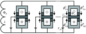
Figure 1: Schematic diagram of the Josephson charge-qubits system. Here $\Phi_{e}$ and $\Phi_{XN}$ represent respectively the magnetic flux crossing electrical inductance $L$ and $N$th SQUID, while $\Phi_{NA(B)}^{L(R)}$ represents the phase Josephson junction. $V_{XN}$ is the voltage through a gate capacitance $C_{N}$.

The considered Josephson charge qubit is realized via a Cooper pair box PRB_36_3548 : a nanometer-scale superconducting island, which is connected via a Josephson junction to a large electrode termed as a reservoir. The typical island dimensions is 1000nm$\times$50nm$\times$20nm (length$\times$width$\times$thickness) and the number of conduction electrons is about $10^{7}-10^{8}$. If the superconducting energy gap is large enough, it will effectively inhibit the particle tunnel effect at low temperature, and it only allows Cooper-pair coherent tunnel effect inside the superconducting Josephson junction. The two symmetric dc SQUIDs are assumed to be identical and have same Josephson coupling energy $E_{Jk}^{0}$ and same capacitance $C_{Jk}$. Since the size of the loop is usually very small $(1\mu m)$, the self-inductance effects of each SQUID loop can be ignored. Each SQUID pierced by a magnetic flux $\Phi_{Xk}$ provides an effective coupling energy given by $-E_{Jk}(\Phi_{Jk})\cos\phi_{kA(B)}$ with $E_{Jk}(\Phi_{Jk})=2E_{Jk}^{0}\cos(\pi\Phi_{Xk}/\Phi_{0})$, where $\Phi_{0}=h/2e$ is the flux quantum. The effective phase drop $\Phi_{kA(B)}$, with the subscript $A(B)$ labeling the SQUID above (below) the island, equals the average value $(\Phi_{kA(B)}^{L}+\Phi_{kA(B)}^{R})/2$ of the phase that drops across the two Josephson junctions in the dc SQUID, where the superscript $L(R)$ denotes the left (right) Josephson junction. The phase drops $\phi_{kA}^{L}$ and $\phi_{kB}^{L}$ are related to the total flux $\Phi=\Phi_{e}+LI$ through the inductance $L$ by the constraint $\phi_{kB}^{L}-\phi_{kA}^{L}=2\pi\Phi/\Phi_{0}$, where $\Phi_{e}$ is the externally applied magnetic flux threading the inductance $L$.

In the muti-qubit circuit, we choose the bases $\{|0\rangle=|n_{i}\rangle$, $|1\rangle=|n_{i}+1\rangle\}$ ($n_{i}$ is the number of electrons in the $i$-th Cooper-pair box), then the Hamiltonian of the system in the spin-1/2 representation can be reduced to

$$\hat{H}=\varepsilon_{i}(V_{Xi})\sigma_{z}^{(i)}-\bar{E}_{Ji}(\Phi_{Xi},\Phi_{e},L)\sigma_{x}^{(i)},$$ (3)

where $\sigma_{x,y,z}$ are Pauli matrices. $\varepsilon_{i}(V_{Xi})=[{C_{i}V_{Xi}}/{e}-(2n_{i}+1)]E_{ci}/2$ is the charge energy that can be controlled via the gate voltage, $E_{ci}=2{e^{2}}/(C_{i}+C_{J0})$. The intrabit coupling $\bar{E}_{Ji}(\Phi_{Xi},\Phi_{e},L)$ can be controlled by both the applied external flux $\Phi_{e}$ through the common inductance, and the local flux $\Phi_{Xi}$ through the two SQUID loops of the $i$-th Cooper-pair box. According to Ref. PRL_89_197902 , $\bar{E}_{Ji}\propto\cos(\pi\Phi_{e}/\Phi_{0})$, we choose $\Phi_{e}=\Phi_{0}/2$ for all boxes in Fig. 1, so that the intrabit coupling is $\bar{E}_{Ji}=0$. We will discuss it in depth in the following text.

The inductance $L$ is shared by the Cooper-pair boxes $i$ and $j$ to form the superconducting loops. The reduced Hamiltonian of the system is given by

$$\hat{H}=\sum_{k=i,j}[\varepsilon_{k}(V_{Xk})\sigma_{z}^{(k)}-\bar{E}_{Jk}\sigma_{x}^{(k)}]+J_{ij}\sigma_{x}^{(i)}\sigma_{x}^{(j)}.$$ (4)

Here the interbit coupling $J_{ij}=-\pi^{2}LE_{Ji}E_{Jj}\sin^{2}(\pi\Phi_{e}/$ $\Phi_{0})/\Phi_{0}^{2}$ is controlled by both the external flux $\Phi_{e}$ and the local fluxes $\Phi_{Xi,Xj}$. For simplicity, we switch $k=2$, so that the Hamiltonian of the system is

$$\hat{H} = [\varepsilon_{1}(V_{X1})\sigma_{z}^{(1)}-\bar{E}_{J1}\sigma_{x}^{(1)}]$$ (5)

$$+[\varepsilon_{2}(V_{X2})\sigma_{z}^{(2)}-\bar{E}_{J2}\sigma_{x}^{(2)}]+J_{12}\sigma_{x}^{(1)}\sigma_{x}^{(2)}.$$

The state of the system at thermal equilibrium can be described by the density operator $\rho=\texttt{exp}(-H/k_{B}T)/Z$, where $Z=\texttt{tr}[\texttt{exp}(-H/k_{B}T)]$ is the partition function with $T$ the temperature, and $k_{B}$ the Boltzmann's constant PRA_66_044305 . We will discuss QD at finite temperatures; this is called thermal QD.

We now propose the methods for achieving the possible maximum value of QD:

(i) The intra-qubit coupling $\bar{E}_{Ji}=0$.

Our numerical results show QD does not exist if the intra-qubit coupling $\bar{E}_{Ji}\neq 0$. Therefore, we only consider the case $\bar{E}_{Ji}=0$ which can be achieved by choosing $\Phi_{e}=\Phi_{0}/2$ for all boxes as $\bar{E}_{Ji}(\Phi_{Xi},\Phi_{e},L)=\xi_{ij}E_{Ji}\cos(\pi\Phi_{e}/\Phi_{0})$. Then the Hamiltonian of the system reduces to $\hat{H}=\varepsilon_{1}(V_{X1})\sigma_{z}^{(1)}+\varepsilon_{2}(V_{X2})\sigma_{z}^{(2)}+J_{12}\sigma_{x}^{(1)}\sigma_{x}^{(2)}$, which is of Ising-like PRB_60_11404 with the "magnetic field" along the $z$ axis. For simplicity, we take $V_{X1}=V_{X2}=V_{X}$ and the Hamiltonian of the system will be

$$\hat{H}=\varepsilon(V_{X})(\sigma_{z}^{(1)}+\sigma_{z}^{(2)})+J_{12}\sigma_{x}^{(1)}\sigma_{x}^{(2)},$$ (6)

the nonzero elements of the density operator $\rho$ are

$$\rho_{11,44}=w_{\mp}/\alpha Z,~{}\rho_{22}=\rho_{33}=\cosh(\beta J)/Z,$$

$$\rho_{23}=\rho_{32}=-\sinh(\beta J)/Z,$$

$$\rho_{14}=\rho_{41}=-\gamma/\alpha Z,$$ (7)

where $w_{\mp}=J_{12}^{2}[\lambda^{2}\cosh(\beta\lambda)\mp 2\varepsilon\lambda\sinh(\beta\lambda)]$, $\alpha=J_{12}^{4}-12\varepsilon^{4}$,$\gamma=J_{12}^{3}\lambda\sinh(\beta\lambda)$, $\lambda=\sqrt{4\varepsilon^{2}+J_{12}^{2}}$, and $Z=2\cosh(\beta\lambda)+2\cosh(\beta J_{12})$.

(ii) The relationship between $J_{12}$ and $\varepsilon$.

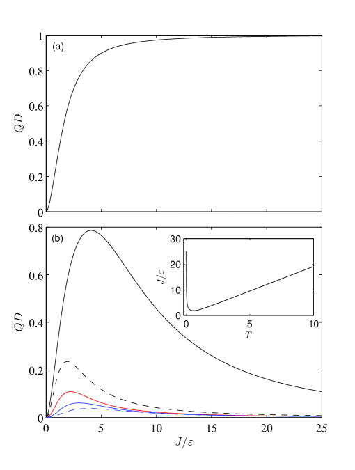
Figure 2: QD versus $J_{12}/\varepsilon$. (a) shows the case of $k_{B}T=0$, while in (b) the lines from top to bottom correspond respectively to the cases of $k_{B}T=0.1K$, $0.5K$, $1K$, $1.5K$, and $2K$. The inset shows that the dependence of the critical $J/\varepsilon$ (when QD attains a certain maximum) on $T$.

For $k_{B}T=0$, QD reaches its maximum value 1 asymptotically with the increase of $J_{12}/\varepsilon$, see Fig. 2(a). For instance, QD is about 0.9988 when $J_{12}/\varepsilon=25$. We display the corresponding results in Fig. 2(b) for the nonzero temperature case, from which one can see that the QD decreases with the increase of $k_{B}T$. For any fixed nonzero $k_{B}T$, a certain maximum QD is achieved at a critical $J_{12}/\varepsilon$ that depends on the temperature. See the inset of Fig. 2(b), the critical $J_{12}/\varepsilon$ decays with $T$ at the low temperature region, and then $J_{12}/\varepsilon$ is discovered to be increased with the increase of $T$. This phenomenon implies that the weak coupling is better for generating the maximum QD in the low temperature region, while the case is opposite in the high temperature region.

III.1 equal magnetic flux $\Phi_{X1}=\Phi_{X2}$

A small-size inductance can be made with Josephson junctions. By fixing some system parameters one can see how the other parameters affect variations of the thermal QD and EoF. In accordance with Ref. PRL_89_197902 , we choose $L=30nH$. Since $J_{12}=-(4\varepsilon_{0}^{2}\pi^{2}L/\Phi_{0}^{2})\cos(\pi\Phi_{X1}/\Phi_{0})$ $\cos(\pi\Phi_{X2}/\Phi_{0})$, $2k\pi\leq\Phi_{X1,2}/\Phi_{0}\leq 2(k+1)\pi$, $(k=0,1,2,...)$. We also chose the junction capacitance $C_{J0}=10^{-5}F$, and used a small gate capacitance $C=10^{-6}F$ to reduce the coupling of the environment. Using $\varepsilon(V_{X})=[{CV_{X}}/{e}-(2n+1)]E_{c}/2$, $E_{c}=2{e^{2}}/(C+C_{J0})$, we can get $V_{X}>10^{-6}V$ while QD decreases with the increase of $V_{X}$.

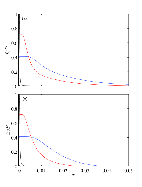
Figure 3: (a) Temperature dependence of QD (a) and EoF (b), with $L=30nH$, $\Phi_{Xi}/\Phi_{0}=0$, and the black, red, and blue lines correspond to $V_{X}=7.5\mu V,50\mu V$, and $100\mu V$, respectively.

Fig. 3(a) is the dependence of QD on temperature $T$ with $\Phi_{X1}=\Phi_{X2}=0$. Clearly, the QD decreases with the increase of $T$ and this tendency is somewhat similar to that of EoF as shown in Fig. 3(b). But the EoF diappears suddenly when $T$ reaches a critical point, which is called entanglement sudden death (ESD) Science_323_5914 . The critical temperature increases with the increase of $V_{X}$. The reason for this behavior is due to the mixing of the maximally entangled state with the other states, while at the same time the thermal QD approaches asymptotically to zero if the temperature is very high. The essence of this interesting phenomenon is that the role of thermal fluctuations exceeds quantum cases as the temperature grows. From Ollivier and Zurek's argument PRL_88_017901 , we know that the absence of entanglement does not mean classicality. The noisy environments can destroy the quantumness of a system and degenerate it to a classical case aop1 . QD measures total quantum correlations and it will not disappear even with very high temperature. From this point one can conclude that QD is more robust than entanglement aop1 .

If the thermal fluctuation is very strong, then the effects of $V_{X},\ L$, and $\Phi_{Xi}/\Phi_{0}$ will become very weak. Now, we will show how $V_{X}$ and $\Phi_{Xi}/\Phi_{0}$ affect the thermal QD for the weak thermal fluctuation case with $L=30nH$. From Fig. 4 with $V_{X}=20\mu V$, one can see that both the thermal QD and the entanglement behave as periodic functions of $\Phi_{Xi}/\Phi_{0}$. The larger the value of $V_{X}$, the lower the amplitude of thermal QD and EoF and they show the same periodic functions. This phenomena can be interpreted by $J_{12}\propto\cos(\pi\Phi_{X1}/\Phi_{0})\cos(\pi\Phi_{X2}/\Phi_{0})$, $\Phi_{Xi}/\Phi_{0}=\theta$. The QD gets its maximum value at the ground state (the black line) when $\Phi_{Xi}/\Phi_{0}=k~{}$ ($k\in\mathbb{N}$). For the thermal states, the QD still presents periodic variations, but its maximum is reduced when $\Phi_{Xi}/\Phi_{0}\neq k~{}$ ($k\in\mathbb{N}$). From the aforementioned example, one can see that in order to achieve the needed QD, then the range of $\Phi_{Xi}/\Phi_{0}$ in one cycle is enough.

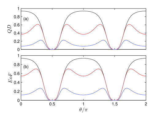
Figure 4: QD (a) and EoF (b) versus $\Phi_{Xi}/\Phi_{0}=\theta$ with $L=30nH$, $V_{Xk}=20\mu V$. The lines from top to bottom correspond to $T=0K$, $T=1\times 10^{-3}K$, and $T=5\times 10^{-3}K$, respectively.

III.2 unequal magnetic flux $\Phi_{X1}\neq\Phi_{X2}$

Figure 5: QD versus $\theta_{1}=\Phi_{X1}/\Phi_{0}$ and $\theta_{2}=\Phi_{X2}/\Phi_{0}$ with $L=30nH$ and $V_{X}=20\mu V$ for $T=0$ (a) and $T=0.01K$ (b).

In Section 3.1 we considered $\Phi_{X1}\doteq\Phi_{X2}$ and here we consider $\Phi_{X1}\neq\Phi_{X2}$. For the ground state at $k_{B}T=0$ and $V_{X}=20\mu V$, one can obtain the analytical formulas

$$D(\rho)=-u\log_{2}u-v\log_{2}v,$$ (8)

where $u={(2\varepsilon+\lambda)^{2}}/{\zeta}$, $v={J^{2}}/{\zeta}$, $\zeta=J^{2}+(2\varepsilon+\lambda)^{2}$. In Fig. 5(a), if $\theta_{1}=\Phi_{X1}/\Phi_{0}$ and $\theta_{2}=\Phi_{X2}/\Phi_{0}$ change synchronously, when $k-\frac{1}{2}\leq\theta_{1,2}\leq k$  ($k\in\mathbb{N^{+}}$), QD increases with the increase of $\theta_{1,2}$; when $k\leq\theta_{1,2}\leq k+\frac{1}{2}$  ($k\in\mathbb{N^{+}}$), QD decreases with the increase of $\theta_{1,2}$. If $\theta_{1}$ and $\theta_{2}$ change asynchronously when $k-\frac{1}{2}\leq\theta_{1}\leq k$  ($k\in\mathbb{N^{+}}$), QD decreases with the increase of $\theta_{2}$ when $k\leq\theta_{2}\leq k-\frac{1}{2}$  ($k\in\mathbb{N^{+}}$); when $k\leq\theta_{1}\leq k+\frac{1}{2}$  ($k\in\mathbb{N^{+}}$), QD increases with the increase of $\theta_{2}$ when $k-\frac{1}{2}\leq\theta_{2}\leq k$  ($k\in\mathbb{N^{+}}$). We explain this phenomenon by analyzing the expression of QD in Eq. (8). When $V_{X}$ and $L$ are constant, QD is only the function of $\Phi_{X1,2}$, which can be obtained from $J_{12}=-(4\varepsilon_{0}^{2}\pi^{2}L/\Phi_{0}^{2})\cos(\pi\Phi_{X1}/\Phi_{0})\cos(\pi\Phi_{X2}/\Phi_{0})$. For thermal states, the curves in Fig. 5(b) and Fig. 4(a) have similar tendency, but QD is very small when $T=0.01K$ and this is clearly not the desired result. Thus, in order to obtain an ideal QD in the ground state one should try to make $\Phi_{Xi}/\Phi_{0}=0$, while to obtain the maximum QD in the thermal states one needs to adjust the system parameters according to the actual situation.

IV Conclusion

In conclusion, one can make the values of QD as large as possible by adjusting the parameters of our two qubits Josephson charge system. For example, by taking $V_{Xk}=20\mu V,L=30nH,\Phi_{X1,2}/\Phi_{0}=k\pi,~{}(k=0,1,2,...)$, the QD approaches approximately to the maximum value 1 for the ground state case at $k_{B}T=0$.

Considering the effect of temperature $T$, thermal QD is more robust than thermal entanglement. For example, thermal entanglement undergoes sudden death while thermal QD does not. In theory, by taking proper system parameters, one can always find a feasible value of QD to help the experimenter to process the quantum information. We hope our research findings demonstrated in this paper will be experimentally realized in the future.

ACKNOWLEDGMENTS

This work was supported by NSFC under Grant Nos. 11104217, 11174165 and 11275099. Shang thanks M.-L. Hu for his warmhearted discussion.

References

- (1) R. Horodecki, P. Horodecki, M. Horodecki, K. Horodecki, Rev. Mod. Phys. 81, 865 (2009).
- (2) M. L. Hu, Ann. Phys. (NY) 327, 2332 (2012).
- (3) M. L. Hu, Phys. Lett. A 375, 922 (2011).
- (4) M. L. Hu, Phys. Lett. A 375, 2140 (2011).
- (5) E. Knill, R. Laflamme, Phys. Rev. Lett. 81, 5672 (1998).
- (6) B. P. Lanyon, M. Barbieri, M. P. Almeida, A. G. White, Phys. Rev. Lett. 101, 200501 (2008).
- (7) H. Ollivier, W. H. Zurek, Phys. Rev. Lett. 88, 017901 (2001).
- (8) L. Henderson, V. Vedral, J. Phys. A 34, 6899 (2001).
- (9) A. Datta, A. Shaji, C. M. Caves, Phys. Rev. Lett. 100, 050502 (2008).
- (10) K. Modi, T. Paterek, W. Son, V. Vedral, M. Williamson, Phys. Rev. Lett. 104, 080501 (2010).
- (11) G. L. Giorgi, B. Bellomo, F. Galve, R. Zambrini, Phys. Rev. Lett. 107, 190501 (2011).
- (12) S. Luo, S. Fu, Phys. Rev. Lett. 106, 120401 (2011); S. Luo, Phys. Rev. A 77, 022301 (2008).
- (13) M. L. Hu, H. Fan, Ann. Phys. (NY) 327, 2343 (2012).
- (14) A. K. Pati, M. M. Wilde, A. R. Usha Devi, A. K. Rajagopal, Sudha, Phys. Rev. A 86, 042105 (2012).
- (15) M. L. Hu, H. Fan, Phys. Rev. A 87, 022314 (2013).
- (16) M. L. Hu, H. Fan, Phys. Rev. A 88, 014105 (2013).
- (17) K. Modi, A. Brodutch, H. Cable, T. Paterek, V. Vedral, Rev. Mod. Phys. 84, 1655 (2012).
- (18) T. Werlang, G. Rigolin, Phys. Rev. A 81, 044101 (2010).
- (19) Y. X. Chen, S. W. Li, Phys. Rev. A 81, 032120 (2010).
- (20) G.-F. Zhang, H. Fan, A.-L. Ji, Z.-T. Jiang, A. Abliz, W.-M. Liu, Ann. Phys. (NY) 326, 2694 (2011).
- (21) J. S. Xu, X. Y. Xu, C. F. Li, C. J. Zhang, X. B. Zou, G. C. Guo, Nat. Commun. 1, 7 (2010).
- (22) M. L. Hu, H. Fan, Ann. Phys. (NY) 327, 851 (2012).
- (23) M. L. Hu, D. P. Tian, Ann. Phys. (NY) 343, 132 (2014).
- (24) F. F. Fanchini, L. K. Castelano, A. O. Calderia, New J. Phys. 12 073009 (2010).
- (25) R. C. Ge, M. Gong, C. F. Li, J. S. Xu, G. C. Guo, Phys. Rev. A 81, 064103 (2010).
- (26) D. O. Soares-Pinto, L. C. Céleri, R. Auccaise, F. F. Fanchini, E. R. deAzevedo, J. Maziero, T. J. Bonagamba, R. M. Serra, Phys. Rev. A 81, 062118 (2010).
- (27) T. K. Chuan, J. Maillard, K. Modi, T. Paterek, M. Paternostro, M. Piani, Phys. Rev. Lett. 109, 070501 (2012).
- (28) B. Dakic, Y. O. Lipp, X. S. Ma, M. Ringbauer, S. Kropatschek, S. Barz, T. Paterek, V. Vedral, A. Zeilinger, C. Brukner, P. Walther, Nat. Phys. 8, 666 (2012).
- (29) M. Gu, H. M. Chrzanowski, S. M. Assad, T. Symul, K. Modi, T. C. Ralph, V. Vedral, P. K. Lam, Nat. Phys. 8, 671 (2012).
- (30) C. Zhang, S. Yu, Q. Chen, C. H. Oh, Phys. Rev. A 84, 032122 (2011); R. Auccaise, J. Maziero, L. C. Celeri, D. O. Soares-Pinto, E. R. deAzevedo, T. J. Bonagamba, R. S. Sarthour, I. S. Oliveira, R. M. Serra, Phys. Rev. Lett. 107, 070501 (2011).
- (31) J. Clarke, F. K. Wilhelm, Nature 453, 1031 (2008).
- (32) J. Q. You, J. S. Tsai, F. Nori, Phys. Rev. Lett. 89, 197902 (2002).
- (33) Y. X. Liu, J. Q. You, L. F. Wei, C. P. Sun, F. Nori, Phys. Rev. Lett. 95, 087001 (2005).
- (34) Y. X. Liu, C. P. Sun, F. Nori, Phys. Rev. A 74, 052321 (2006).
- (35) J. Majer, J. M. Chow, J. M. Gambetta et al., Nature 449, 443 (2007).
- (36) C. H. Bennett, D. P. DiVincenzo, J. A. Smolin, W. K. Wootters, Phys. Rev. A 54, 3824 (1996);
- (37) W. K. Wootters, Phys. Rev. Lett. 80, 2245 (1998).
- (38) M. Büttiker, Phys. Rev. B 36, 3548 (1987); V. Bouchiat, D. Vion, P. Joyez, D. Esteve, M. H. Devoret, Phys. Scr. T76, 165 (1998).
- (39) X. G. Wang, Phys. Rev. A 66, 044305 (2002); Y. Sun, Y. G. Chen, H. Chen, Phys. Rev. A 68, 044301 (2003); G. F. Zhang, S. S. Li, Phys. Rev. A 72, 034302 (2005).
- (40) G. Burkard, D. Loss, D. P. DiVincenzo, J. A. Smolin, Phys. Rev. B 60, 11404 (1999).
- (41) T. Yu, J. H. Eberly, Science 323, 5914 (2009).